Abstract.
Twin-to-twin transfusion syndrome is a condition in which identical twins share a certain pattern of vascular connections in the placenta. This leads to an imbalance in the blood flow that, if not treated, may result in a fatal outcome for both twins. To treat this condition, a surgeon explores the placenta with a fetoscope to find and photocoagulate all intertwin vascular connections. However, the reduced field of view of the fetoscope complicates their localization and general overview. A much more effective exploration could be achieved with an online mosaic created at exploration time. Currently, accurate, globally consistent algorithms such as bundle adjustment cannot be used due to their offline nature, while online algorithms lack sufficient accuracy. We introduce two pruning strategies facilitating the use of bundle adjustment in a sequential fashion: (1) a technique that efficiently exploits the potential of using an electromagnetic tracking system to avoid unnecessary matching attempts between spatially inconsistent image pairs, and (2) an aggregated representation of images, which we refer to as superframes, that allows decreasing the computational complexity of a globally consistent approach. Quantitative and qualitative results on synthetic and phantom-based datasets demonstrate a better trade-off between efficiency and accuracy.
Keywords: mosaicking, fetoscopy, electromagnetic, twin-to-twin transfusion syndrome, drift-free, efficient
1. Introduction
Twin-to-twin transfusion syndrome (TTTS) is a fetal condition that affects monochronic diamniotic pregnancies in which the presence of a certain pattern of intertwin vascular connections, known as anastomoses, results in an imbalance of the blood flow between twins. If this condition remains untreated, the outcome is generally fatal for both twins.1 Minimally invasive surgery is today the standard of care. The surgeon explores the placenta using a fetoscope with a small field of view to find and photocoagulate all anastomoses. Despite the wide literature in endoscopic scenarios,2,3 the challenges found in fetoscopic imagery complicate the application of available techniques. To illustrate the complexity of the fetoscopic site, Fig. 1 shows three examples of TTTS procedure where the reduced field of view can be observed. The surgeon must remember the explored areas to navigate through the placental surface building a mental map of the placenta. This is an extremely challenging task even for the best-trained surgeons due to this limited field of view, lack of texture, and turbidity, which hinders the visualization and also precludes any assistance from others. As a solution, mosaicking has been suggested to increase the field of view by stitching the images together in a common space, forming a map of the area.
Fig. 1.
Three examples of images taken in clinical conditions from a TTTS surgery.
The online creation of such map would allow for a more effective exploration4,5 and localization of the anastomoses. Online approaches for mosaicking6–8 usually rely on approximations that either summarize past information or do not make use of all available information. In some applications, a simple pairwise estimation,5,9 where subsequent images are registered, can be appropriate for real-time operation. However, these approaches accumulate drift.
To mitigate the drift, a globally consistent method might be used. Bundle adjustment10 is considered to be the offline reference method in globally consistent mosaicking due to its accuracy, which comes from the effective use of all the available information in a probabilistic way. When the number of frames increases, however, the limitations in computational complexity become more evident, and online operation becomes prohibitive.
In Ref. 6, the authors proposed to use an electromagnetic tracker (EMT) to guide the estimation and mitigate the drift. However, due to their computational complexity or suboptimality, the proposed strategies were not suitable to obtain accurate online mosaics with clinically acceptable update times.
Some efforts have been made to reduce the computational time of globally consistent approaches. For example, Schroeder et al.11 proposed closed-form initial estimates to accelerate its convergence. Steedly et al.12 used the concept of keyframes in an offline setting to denote a set of the most important frames; an all-to-all strategy analogous to bundle adjustment is used with the keyframes whereas a pairwise web connects the rest of frames enforcing only local consistency between them. This permits to reach mosaics of the order of thousands of frames. Despite the computational advantage of this approach, the reduction in the number of connections between nonkeyframe images leads to a decrease in robustness given that not all the information available has been used. The use of the redundancy provided by nonkeyframe images becomes essential when dealing with fetoscopic images due to their relatively poor quality.
An alternative to Ref. 12 consists of matching exclusively the images that are highly likely to share visual corresponding points, avoiding incoherent attempts. A proposed technique for overlap detection in monocular systems is to use a bag of words13 (BoW), which creates a dictionary of visual words and assigns a signature per image. This signature summarizes the number of occurrences of the visual words in a histogram. In the case that the scene is revisited, the signature of the current image is very similar to the signature of the images initially acquired. However, this strategy works in an offline fashion while we aim for a sequential approach. This is the case for the work of Garcia-Fidalgo et al.14 where an incremental BoW approach is used. However, pose information provided by an EMT system is much stronger than visual information in the placenta given that some uniform textureless areas of the placenta can lead to challenging scenarios. Therefore, we propose to use the EMT system to infer the topology of the cameras imaging the scene.
The organization of this paper is as follows: In Sec. 2, we review the background in mosaicking using the EMT system, to further detail our methodological contributions. The presentation of our experimental suite is done in Sec. 3, demonstrating a decrease in the computational complexity of bundle adjustment while maintaining similar accuracy. Then, we comment on the results in Sec. 4 and conclude the study in Sec. 5.
2. Methods
In this section, we present the preliminary background to then detail our algorithms. We start by introducing the scenario and stating the assumptions made to simplify the problem throughout the paper.
-
•
We consider a placenta to be a plane. In Ref. 15, the authors demonstrated that this assumption greatly simplifies the problem.
-
•
We assume the placenta to be static.
-
•
Despite the image is obtained using a fetoscope, we use a pinhole camera model.13,15
-
•
The EMT field is not perfect. Yet, we assume we are working on the center of the field, and that therefore, that the distortions due to inhomogeneities in the electromagnetic field are neglibible.6
-
•
We assume6 the each EMT measurement to be centered on the true measurement , with a multivariate Gaussian noise of covariance matrix .
We now introduce some concepts that are essential for the rest of the paper: how the visual aligned is performed in a pairwise and globally consistent manner, the link between poses and their imaged scenes over a planar surface, and how the EMT system can be introduced into the mosaicking pipeline.
2.1. Background in Mosaicking
Given a sequence of images , the goal of mosaicking is to find a two-dimensional representation of the scene or mosaic (RGB) where is denoted the mosaic space. Provided that the camera observes a planar scene, a homography exists between corresponding points in two views , , which lie in their respective image spaces , . This homography can be parametrized as a matrix such that
| (1) |
Then, Eq. (1) can be written as where is defined up to scale and the tilde indicates that the points are expressed in homogeneous coordinates.16
If the same planar scene is observed from both views, a homography can be directly inferred from image matching information.17 In this work, we use a landmark-based registration approach18–20 since these approaches usually allow for sparse feature detection which can be faster than using the information in the whole image.
Pairwise mosaicking (PM) relies on estimations of pairwise homographies which project any point from the space of image onto the space of image . Pairwise homographies are then used to compose homographies from a fixed reference, which without loss of generality, can be placed on the first frame as
| (2) |
where the product operator denotes the left matrix multiplication, corresponding to the composition of homographies, e.g., . Once the homographies relating every frame to the reference are computed, every pixel in every image is projected onto the mosaic space. To further clarify the nomenclature, we name absolute homographies with a single subindex meaning that they project any point from the reference to the image frame space , whereas pairwise homographies are defined as mapping points from to . When performing PM, any residual error in the estimation of pairwise homographies is accumulated through the chain in Eq. (2), resulting in a wrong placement of the images in the mosaic that degenerates in an uncontrolled way over time.
Globally consistent approaches such as bundle adjustment10 take into account the relationship between all pairs of images in the sequence to create globally consistent mosaics.21 However, they are generally not fast enough for online operation; the main reasons are the acquisition of the correspondences between all images and the run-time of the nonlinear optimization procedure.
Let us define as the set of all pairs of image indices in which correspondences have been successfully acquired. We aim to obtain a set of estimated homographies , where the hat denotes that they are an estimate, that minimizes the reprojection errors of the matching points in all images in the sequence, namely:
| (3) |
is the number of matches found in the pair , is the conversion from homogeneous to Cartesian coordinates so that , and is the variance associated with the location of a feature once propagated to the space of its matched pair. This variance is associated with the fact that we model the error between a fixed point in an image, and its corresponding pair propagated from the other image as a Gaussian random variable. Note that, since one frame is defined as the reference (here chosen as the first frame, without loss of generality), we only require to estimate homographies, the remaining one being set to identity.
Let be the set of corresponding true camera poses. In addition, let be the respective EMT measurements of these poses, where we assume to be a noisy instance of the true camera . We parametrize each camera pose as a rotation and translation . The vector is parametrized in the same way. The three-parameter rotation vector is extracted from the skew symmetric matrices , which can be converted into the rotation matrix .22 refers to the special orthogonal group of matrices of dimension with determinant 1, and is its corresponding lie algebra. With a rotation matrix and a translation , we can compose the rigid transformation , where is the special Euclidean group corresponding to rigid transformations in three-dimensional space
| (4) |
A set of camera poses (provided by the EMT system) on their own do not give us enough information to create a mosaic. To that end, a set of homographies is necessary, requiring also the planar structure modeling the scene. We now detail how to obtain a set of homographies from both poses and the surface plane. Provided that only camera poses are measured, we need to establish a link between these and imagery.
Let us consider a virtual camera with its virtual image plane located in the origin of coordinates, which we use as a reference, whose image plane space is . We can then link the spaces of the images obtained by the cameras, and their respective motions provided that the imaged plane is known. Since it is so, there is a homography defined that propagates any point in the virtual image to any other image through the following equation, that for convenience we define as
| (5) |
where is the intrinsic camera calibration matrix, and corresponds to the unit normal vector to the imaged surface observed from the origin of coordinates, divided by the distance between origin of coordinates and the plane
| (6) |
We use this relation in order to relate the visual content in the images with EMT readings of the camera poses. The complete derivation of Eq. (5) can be found in Ref. 16.
In the following work, Ref. 6 introduced a probabilistic graphical model that infers the set of poses and planar structure by solving the minimization problem
| (7) |
where , are the set of estimated camera poses and plane, respectively, the cost represents the sum of all reprojection errors between matching landmarks with pairs of indices found between all images where the homographies , are obtained using the three components; the two camera poses , , and plane as in Eq. (5). The EMT information is incorporated in the second cost as
| (8) |
| (9) |
This prevents the poses to be estimated from drifting provided that the EMT measurements have a common reference, which do not allow drift to separate the cameras from the measured position. In other words, the solution obtained as a result of Eq. (7) reflects a guided estimation of the parameters using the EMT system.
2.2. Pruning Strategies for Sequential Bundle Adjustment
In this section, we present our two pruning strategies: (i) the use of the EMT system to identify and discard nonoverlapping frames for which no matching should be attempted, and (ii) the introduction of the concept of superframe; an extension of a typical frame that allows for more efficient mosaicking schemes. We present two pipelines that increasingly incorporate the contributions mentioned above.
2.2.1. Frame pruning using the EMT system
Given the small field of view in fetoscopy and the relatively large area to explore, only a small subset of images shares visual content. Global alignment schemes typically attempt to find correspondences between each pair of images, although in many cases such as ours, the majority of image pairs do not overlap spatially and thus cannot be matched. A given image will typically only match to a small spatially adjacent subset. For this reason, we propose to use the information of an EMT system to find plausible image candidates, bypassing the computation of unnecessary failed matching attempts and reducing, thereby the computational complexity of bundle adjustment.
At a given time instant , we have the current EMT measurement and the previous estimation of the plane by solving the nonlinear optimization problem posed by Eq. (7). Therefore, we can compute a noisy homography using Eq. (5) as
| (10) |
This estimation of the homography, even if not very accurate, can be used to decide whether two images are likely to overlap, thus allowing to filter out spatially unreasonable candidates. To do so, once the homography is obtained, we project the corners of the bounding box containing the circular fetoscopic region of interest through onto the mosaic space as
| (11) |
where the points and represented in homogeneous coordinates, are the original and propagated image corners to the mosaic space , respectively, where denotes the corner index. Then, the overlap between the current and previous frames can be easily and efficiently obtained. Kekec et al.8 showed how this problem can be seen as a simple convex polygon intersection problem. The estimation of the overlap given two convex polygons can be efficiently solved using the separating axis theorem (SAT);8 a theorem from computer graphics that states that if a straight line can be drawn between two convex polygons, then the polygons do not overlap.
2.2.2. Pairwise compression
A practical problem in mosaicking12 algorithms is that hundreds of correspondences are typically stored and used in the optimization procedure per image as can be seen in Eq. (9). Instead, we parametrize the pairwise relation as five equivalent correspondences in the following way: (i) after the pairwise homography estimation using RANSAC simultaneously with the correspondences acquisition,17 we take the bounding box that includes all the interest points in the image. In particular we take the top-centered, bottom-centered, left, and right point locations as well as the center of the bounding box to account for the spread of these points in the original image space. (ii) We propagate them using the estimated homography that relates both images to obtain the second set of points, which completes the collection of correspondences. These correspondences will then be kept for the optimization, reducing the run-time of the cost function greatly.
The more correspondences we acquire, the more correspondences must be taken into account in the cost function. This might not be a problem at the beginning of the sequence, but as the number of correspondences increases, the computational cost increases as well, hindering online operation. We now introduce an additional strategy that generalizes a regular frame in a more efficient representation for mosaicking.
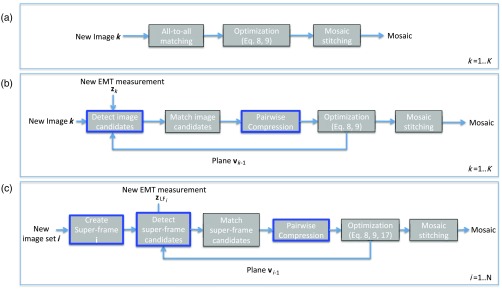
Figure 2(a) shows the proposed pipeline proposed in this section while Fig. 2(b) shows the diagram of the pipeline proposed in Sec. 2.2.3. In both pipelines, the pairwise compression mentioned in Sec. 2.2.2 is applied. Contributions to the mosaicking pipeline are outlined with a blue border.
Fig. 2.
(a) Pipeline proposed in Sec. 2.2.1 using the EMT system to filter out incoherent matching attempts. (b) Pipeline proposed in Sec. 2.2.3 using the superframe. In both pipelines, the pairwise compression mentioned in Sec. 2.2.2 is applied. Contributions to the mosaicking pipeline are outlined with a blue border.
2.2.3. Superframe representation
The superframe representation is a generalization of a frame that incorporates one or more frames. The main idea is to partition the image set into subsets of images grouped into superframes with . Since it is a generalization of an image, the superframe can be incorporated into the standard bundle adjustment pipeline reducing its computational burden drastically. Let us formally define the concept of superframe.
We define a superframe as a representation of a subset of frames that encodes the most salient information of the region observed by all images in the superframe which are indexed by . A lead image with index is defined as the central image in the superframe of window of size , being an integer. If the lead image was taken in isolation, then this would be equivalent to the concept of keyframes.12 In contrast, the superframe uses information of all the images in the window.
Analogously to the standard pipeline, interest point locations and descriptors are extracted for all frames within each superframe. We propose to use the lead image space as a common space where all interest points in the superframe lay, defining the superframe as . To propagate the locations of interest points into this common space, we define as a matrix containing all point locations in homogeneous coordinates, where is the number of interest points found in image . If expressed this way, the points can be propagated onto the lead image space as
| (12) |
while the descriptors are grouped as
| (13) |
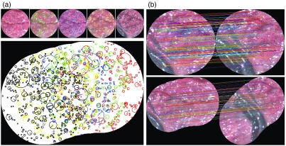
where the homography is the homography that relates the frame within the superframe with the lead frame . This homography is obtained by first running a local, small-scale visual bundle adjustment with all images following the methodology described in Sec. 2.1. Within the superframe, the aligned homographies are then considered fixed in the rest of the pipeline. Figure 3(a) depicts the process of the creation of a superframe, and Fig. 3(b) shows the differences in matching between two images (top) and two superframes (bottom).
Fig. 3.
(a) Creation of a superframe. From top to bottom: images are registered using bundle adjustment10 and their interest points are propagated to the space of the lead frame , forming a superframe. (b) Matching of two frames (85 inliers) and two superframes (165 inliers).
2.2.4. Superframe in the mosaicking pipeline
To integrate the superframe into the mosaicking pipeline, we extend the probabilistic framework6 summarized in Sec. 2.1. However, now superframes replace single frames. To highlight why this is possible, let us describe the simple scenario where two superframes are created. In that case, their descriptors can be matched directly since the input to the matching algorithm is two sets of descriptors. From there, the matching process is analogous to the one described in the PM in Sec. 2.1. Figure 2(c) shows the diagram of the pipeline using the superframe, marking in blue the contributions in the pipeline. In applying directly,6 only one EMT measurement is assumed to be associated with each frame. Therefore, there would be EMT measurements unused per superframe. Instead, we propose to modify the pipeline to include all EMT measurements in the window for better placement of the superframe in the mosaic.
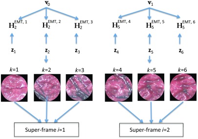
These measurements can be used to obtain homographies using Eq. (5) and the previously estimated resulting from Eq. (7). Figure 4 shows the nomenclature and indexing, displaying each homography composed using the EMT system. Using the EMT measurements and the fixed homographies found in the initial bundle adjustment to build the superframe,, we can obtain measurements of the lead homography coming from each of the EMT measurements in a given superframe as
| (14) |
Fig. 4.
A superframe indexed by is composed of a set of single frames indexed by . Each homography is created from the EMT measurement and the previous plane estimation .
We consider these homographies as measurements of the true homography that places the lead image into the mosaic space, and formulate the problem as
| (15) |
where and are weights. The two first costs are precisely the costs defined before in Eqs. (9) and (8), and the proposed additional term for the global alignment cost function is defined as
| (16) |
| (17) |
where represents control points. Specifically, we used the four corners and the center point of an image as control points. Setting is not trivial since it depends on the accuracy of the EMT system and previous estimation of the normal vector. Therefore, we use it conservatively setting a standard deviation of 10 pixels.
Once all homographies from the mosaic space to the lead frames of each superframe are obtained, one must place the superframes into the mosaic space. To do that, each one of the images within the superframe has to be placed in the mosaic space. Therefore, we must obtain individual homographies for each frame in the sequence that relates it with the mosaic space. One must note, however, that when running bundle adjustment on the superframes, the reference is in the space of the first lead frame, which corresponds to index . For simplicity, we denote the estimated homographies as , skipping the second subindex, which would be . However, one must keep in mind that they are actually from the first lead frame to as . Therefore, to compose a mosaic in the space of the first image, not the first superframe, one must use
| (18) |
Once the absolute set of homographies is obtained, one can project the images onto the mosaic space to be blended.
2.2.5. Efficient implementation of the pipeline using superframes
The main idea of the superframe is to summarize many frames into a region by first performing a local bundle adjustment of frames, each with a complexity of . This entails all-to-all matching of all images within the superframe. On the other side, the complexity of a full bundle adjustment (FBA) is quadratic in the number of frames . By using superframes instead of single frames, one allows reducing the number of effective images used in a general bundle adjustment. This procedure now takes into account superframes, so the total complexity is only where . The first term accounts for the small bundle adjustments of size to build each superframe and then the second term accounts for the complete bundle adjustment of the superframe. For example, in a sequence of frames, where the window , we only have superframes. Therefore, the construction of the superframes would take whereas a single FBA would take , where and are timings related to interest point detection and matching, which differ for single frame and superframe, depending on the number of frames used to create each superframe.
The number of interest points contained in a superframe would be the sum of the number of interest points detected in each image. As increases, this number can quickly become too large and prohibitive for matching. To reduce the number of interest points in the superframe drastically, we put two strategies in place. First, we greedily select only interest points resulting in being inlier matches within every frame in the creation of the superframe. Intuitively, interest points that have already been matched should have a higher probability of being matched in the superframe compared to other points that might not be as well described. The second strategy is to keep a precomputed a KD-tree,23 implementing an approximate nearest neighbors strategy for efficient matching in the creation of the superframe.
In addition, the matching candidate selection strategy mentioned in Sec. 2.2.1 is adapted to be used with superframes instead of single frames. To apply it, only the meaning of overlap for two superframes has to be redefined: two superframes overlap if any of their single frames overlap. In this way, we can incorporate the computational advantage of using superframes that leverage the EMT system to filter out spatially incoherent matching candidates.
3. Experiments
In this section, we present our experimental suite to demonstrate the computational advantage of the proposed pruning strategies compared against a baseline implementation of bundle adjustment. We start by presenting the datasets, algorithms, metrics, and implementation details.
3.1. Datasets
We generated two datasets formed by a set of images and EMT data; synthetic (SYN, 273 frames, ) and a phantom based (PHB, 701 frames, ) datasets. SYN is a translation-based raster scan generated by simulating ground truth camera motions, from which EMT measurements are generated by applying Gaussian noise,6 and for which the images were extracted as projections of the scene observed by the cameras. In that case, the scene consisted of a planar, high-resolution digital image. PHB was recorded by imaging a printed image of a placenta. The setup consisted of a camera head IMAGE1 H3-Z SPIES mounted on a 3-mm straight scope 26007 AA 0° (Karl Storz Endoskope, Tuttlingen, Germany), an EMT system NDI Aurora with a planar field generator, and a Mini 6 DoF sensor. A collection of homographies by semiautomated registration of each fetoscopic image to the original image of the placenta, where a landmark-based approach was used to align the images after the initial manual alignment.
3.2. Algorithms
As a baseline, we compare our algorithms to both the established FBA as well as the standard PM approach, which is very fast but accumulates drift. We apply the matching compression strategy presented in Sec. 2.2.2 as well as the use of the EMT system to discard inconsistent matching attempts (SAT). Our second contribution is the introduction of the superframe (SF) and its incorporation to the mosaicking pipeline. By default, we have chosen . We explicitly name to a run where corresponds to the size of the window used in the superframe.
3.3. Metrics and Implementation Details
We compare the homography and the ground truth homography by computing the mean residual error of a projected grid of points from the image space to the mosaic space. Then, the error between two mosaics is computed as the mean of individual errors . This error is defined in the mosaic space, which is the space in which the final composition is performed. Note that we use with superindex to refer to the residual error between two sequential mosaics at each time instant whereas with subindex refers to the error of the alignment of a single image . To make this metric independent to the choice of reference space, we compute the average of the errors using all images as a reference, as in
| (19) |
In terms of feature-based method, we used SURF.20 The matching was performed using fast approximate nearest neighbors.23 The fetoscope was precalibrated using the Matlab Camera Calibration Toolbox. We also precomputed and applied the Hand-eye Calibration24 matrix from a sequence of images of a checkerboard as well as synchronized sensor poses. The window size of the superframe was determined from the trade-off analysis as , which is presented later in Sec. 3.3. In addition, given that superframes contain many more correspondences than actual frames, a kd-tree23 can be trained and stored per superframe. Then, fast approximate nearest neighbor can be used to accelerate the matching between superframes. The experiments have been performed in an Ubuntu 16.04 with Intel Core I7 at 2.5 GHz and 6 GB of memory.
Next, we evaluate sequential bundle adjustment and evidence the decrease in computational time that the proposed strategies provide.
3.4. Speedup: Correspondence Acquisition
In this section, we analyze the computational cost of a sequential bundle adjustment in an online setting. More precisely, we focus on correspondence acquisition.
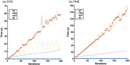
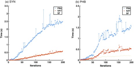
In Fig. 5, we display the run-time of correspondences acquisition in the three algorithms for both datasets. As expected, SAT is faster than FBA in both cases, and SF shows the best in terms of computational cost. In the case of the phantom-based dataset, we can observe that SAT is not necessarily faster all the time. This is due to the trajectory that the camera has followed in this particular dataset. If the overlap between images is too large, then the algorithm suggests all images as possible candidates.
Fig. 5.
Runtime of the correspondences acquisition with respect to the number of iterations for both SYN and PHB datasets.
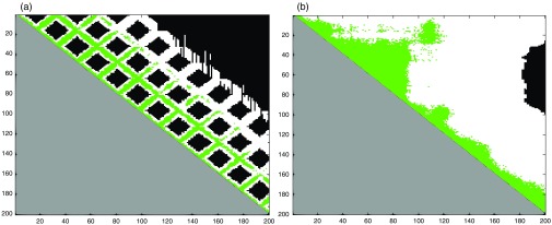
To further evidence where the computational savings have happened spatially, we analyze the percentage of potential image candidates that have been selected using an occupation matrix. This matrix shows whether there has been a match from image (corresponding to row ) to image (corresponding to column ). For a more informative representation, we have color-coded the matrices. Out of all image matches that would have been obtained using an FBA (white), only a portion of them would be selected by SAT (green). Due to the use of symmetrical matching, we only display the upper right triangle in the occupancy matrix. Figure 6 shows that, in the case of SYN (a), 100% of the proposed candidates are correct, and no matches have been missed, saving a total of 54.2% matching attempts. As mentioned before, the path followed by the camera in the PHB [Fig. 6(b)] makes saving matching attempts more complicated. 100% of the proposed candidates are correct; however, there is only a total saving of 5.2% attempts, which happened to be toward the end of the sequence.
Fig. 6.
Occupancy matrix. The pixel shows a color-coded outcome of the matching process. Potential matching candidates are in white. Proposed candidates that have been matched are in green. Black pixels reflect that no candidate was selected but there was no real match. Occupation matrices in (a) the synthetic dataset (SYN) and (b) the phantom-based dataset (PHB).
We now study the run-time of the nonlinear optimization as the second bottleneck for bundle adjustment to reach sequential operation.
3.5. Speedup: Nonlinear Optimization
The computational cost of the nonlinear optimization is due to the run-time of the cost functions in Eqs. (9) and (8) and the number of iterations to convergence. In contrast to standard bundle adjustment where we do not have any initial estimate a priori, subsequent estimations can be used as an initial estimate in a sequential version of bundle adjustment, providing a speedup at each iteration due to the proximity to the minimum. Although this is a desirable property, the question that might prevent desirable update rates is whether the number of iterations to convergence grows with time.
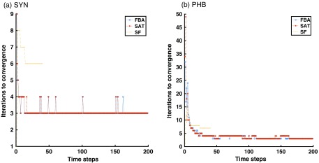
In Fig. 7, we show the number of iterations to convergence in both SYN and PHB datasets.
Fig. 7.
Number of iterations of the nonlinear optimization procedure for FBA, SAT, and SF.
The fact that the approaches show a constant tendency over time is crucial since it indicates that the number of iterations in the nonlinear optimization does not seem to be a bottleneck for offline operation. Given the textureless nature of fetoscopic images, using only a subset of all frames is not a very robust option. Instead, we would like to use the redundancy in the complete video sequence. Figure 8 shows the optimization times for FBA, SAT, and SF. It can be seen how if compression is used (SAT), the slope decreases with the number of iterations. Now that we have demonstrated the decrease in computational burden in the proposed algorithms, we need to evaluate their accuracy and show that despite the improvement in speed, there is no significant loss in accuracy.
Fig. 8.
Runtime of the nonlinear optimization for FBA, SAT, and SF.
3.6. Efficiency
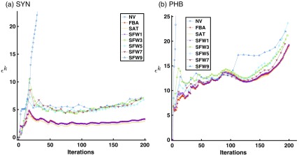
In this section, we analyze the performance of the proposed algorithms for classical pipelines. In particular, we computed the error in each sequential mosaic for NV and FBA as a baseline, comparing it to SAT, and SF with different window sizes in SYN and PHB datasets, respectively. Figure 9 shows the errors for each of the methods. The error in NV spikes from the beginning. This is well known due that there is no global correction and therefore, drift is accumulated. While SF results in the best performance regarding computational advantage, the decrease in accuracy for all the window sizes except for which the behavior should be very similar to SAT. When the window increases, the accuracy of the SF remains stable.
Fig. 9.
Error in NV, FBA, SAT, and SF with a window size of 1, 3, 5, 7, and 9 for SYN and PHB.
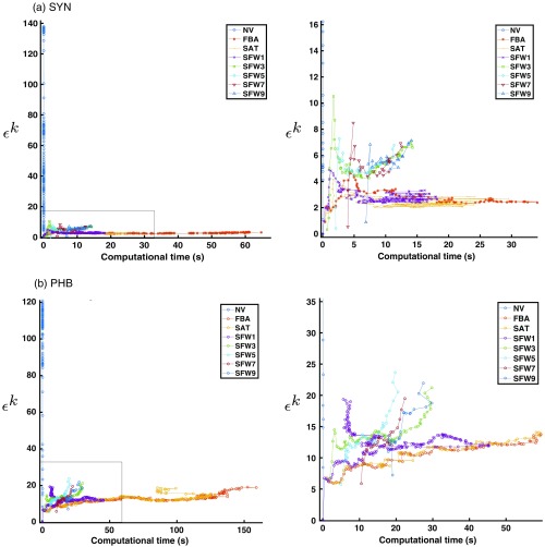
Since the data reflects this trade-off between computational power and accuracy, we propose to analyze this trade-off with the graph in Fig. 10. This graph shows the error in the axis and the time per iteration in the axis. We have plotted each algorithm in a different color. In here, temporal evolution is not shown; however, one can observe the temporal trail by looking at the lines connecting the dots, taking into account that first iterations are the fastest. For an efficient algorithm, we would like the error and computational time to be low. Therefore, we identify the most efficient algorithm as the one whose results lie in the bottom left corner. The same tendency can be seen for both datasets; despite being efficient, the NV drifts in large measure, making the algorithm not worth pursuing. The FBA is not a good option concerning the trade-off since the computational time is too large, yet it does keep the accuracy very low. SAT performs similarly, albeit much more efficiently than FBA. On top of that, all versions of SF perform more efficiently than SAT. In particular, we see that as we increase the window size, the efficiency starts to be better until . The selection of the best algorithm is not trivial since shows a faster start yet slower end than in both datasets due to the need for matching more superframes. After this, efficiency starts to fall systematically. We believe that the increase of computational time that takes to perform the first bundle adjustment causes this effect, growing with . Since many of the operations in the creation of the superframe could be performed in parallel, we expect slightly better results for a parallelized version of the approach.
Fig. 10.
The trade-off between the error in the -axis and computational time in the -axis. To the left, a zoomed version of the graph in the right for both (a) SYN and (b) PHB. Each color represents a different algorithm and despite the graph does not aim to show the temporal evolution, the connection between points provide an indication.
In Figs. 11 and 12, we show mosaics for SYN and PHB datasets, respectively, for the NV, FBA, and SFW5. While the figure shows some steps of the sequential estimation of the mosaic, we encourage the reader to visualize the videos included in the supplementary material for a more thorough visualization of the results.
Fig. 11.
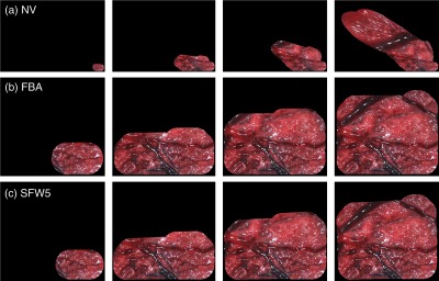
Sequential screenshots of the mosaic using (a) NV, (b) FBA, and (c) SFW5 in the SYN dataset (Video 1, MP4, 1426 KB [URL: https://doi.org/10.1117/1.JMI.6.3.035001.1; Video 2, MP4, 8195 KB [URL: https://doi.org/10.1117/1.JMI.6.3.035001.2; Video 3, MP4, 2447 KB [URL: https://doi.org/10.1117/1.JMI.6.3.035001.3).
Fig. 12.
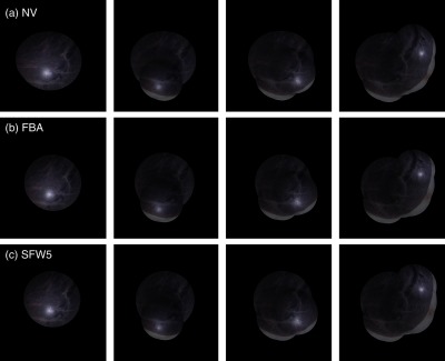
Sequential screenshots of the mosaic using (a) NV, (b) FBA, and (c) SFW5 in the PHB dataset (Video 4, MP4, 2844 KB [URL: https://doi.org/10.1117/1.JMI.6.3.035001.4; Video 5, MP4, 3443 KB [URL: https://doi.org/10.1117/1.JMI.6.3.035001.5; Video 6, MP4, 811 KB [URL: https://doi.org/10.1117/1.JMI.6.3.035001.6).
4. Discussion
Bundle adjustment is in general slow due to the mentioned reasons. In this work, we propose the use of the EMT system to identify potential matching candidates, avoiding unnecessary matching attempts. However, the computational savings will greatly depend on the motion of the camera. For example, if the camera remains in the same position, then the EMT system will determine that all the frames are candidates being equivalent to an all-to-all matching scenario. On the contrary, if the camera moves, the EMT system is able to identify a reduced set of potential candidates. A simple solution to this problem could be set up a preprocessing step of filtering out the frames that overlap more than a certain area threshold.
The accuracy of the EMT is limited. Discarding nonmatching candidates is a process that can be made more loose or aggressive by just increasing or decreasing the size of the images when determining overlapping frames. This will depend on the accuracy of the EMT when projected to the image space, i.e., the noise on the EMT system, but also the camera parameters, and the placement of the planar object. In our datasets, results seem to suggest that taking the image size is enough to discard incoherent matching candidates.
However, the estimation of the overlap is dependent on having a reliable normal estimation. When the camera has not observed enough scene, the estimation of the normal vector is less accurate due to the lack of depth perception in a small baseline. When more parts of the scene are observed, the normal vector converges, and only a few constant number of iterations are necessary for convergence in subsequent iterations. In fact, the results suggest that only a constant number of iterations are enough for the nonlinear optimization to converge. This is a significant result that reveals that the number of steps to convergence is not a problem for achieving clinically feasible update rates. The obvious exception to this point is if there are outliers in an image. If so, then the cost function does not reflect the problem to solve and as a consequence, the number of iterations to converge grows, not reaching the desired minimum. Therefore, it is essential to obtain an outlier-free set of correspondences.
The creation of a superframe requires a first bundle adjustment. This process, even if it takes some time, is compensated by the fact that the general bundle adjustment takes only frames into account. The efficiency gain is expected, whenever, the number of superframes is less than the number of frames . However, errors in the local bundle adjustment impact in the second, global, bundle adjustment since it is only optimizing for the lead frame in the superframe. If there is an error, one of the homographies of the superframe, then the interest points will be erroneously placed within the space of the lead frame in the superframe. Then, a geometrical validation such as RANSAC could filter them out for being geometrically inconsistent with a homographic model. This results in a trade-off between the accuracy and the window size . A second trade-off is that concerning the window size concerning efficiency. When the first bundle adjustment is large, then the number of efficient superframes to optimize in the global bundle adjustment is smaller and vice-versa. However, the larger is the superframe, the more rigid the system is, and this makes it more prone to alignment errors. Also, as the window size is larger, the distance between lead frames also increases and matching becomes more complicated.
In the described case where a fixed window is used, the optimal will greatly depend on the motion on the camera making the choice of the value not trivial. We have chosen as the best trade-off between accuracy and computational cost in the evaluation. An interesting fact is that the accuracy of the mosaic does not seem to decrease much between different instances of superframes even though its computational time does.
We propose a system in which single frames are not shared by the superframes, i.e., each frame index is only in one superframe. However, an interesting research line could be to inspect the impact of incorporating each index in more than one superframe. This implies that the number of frames in the nonlinear optimization procedure grows, trading an increase in the run-time of the algorithm for more robustness.
5. Conclusions
In this work, we propose two different pruning strategies allowing the sequential application of bundle adjustment for mosaicking. To make this possible, we tackle the computational bottlenecks of bundle adjustment using two different pruning strategies. First, we use the EMT system to discard a high percentage of spatially inconsistent matching attempts. Second, we introduce the concept of superframe and introduce it into the mosaicking pipeline. This concept is a generalization of an image, which can be used to reduce the computational complexity drastically in both the correspondence acquisition and optimization phases. We show a large decrease in computational complexity with respect to a standard bundle adjustment, on both synthetic and phantom-based datasets. This makes possible the use of a sequential bundle adjustment, which achieves a better compromise between efficiency and accuracy than standard approaches. The results of this work open new avenues to online operation, leading the state of the art in online mosaicking one step closer to clinical translation.
Supplementary Material
Acknowledgments
This work was supported by the Welcome Trust (WT101957; 203148/Z/16/Z; 203145Z/16/Z) and EPSRC (NS/A000027/1; NS/A000049/1; NS/A000050/1; EP/L016478/1). Jan Deprest was being funded by the Great Ormond Street Hospital Charity.
Biographies
Marcel Tella-Amo is a PhD student at the University College of London (UCL). He also received his MRes in medical imaging at UCL in 2016. Previously, he received his BE + MSc degree in telecom engineering focused on image processing at the Technical University of Catalonia (UPC), Barcelona. His research interests include machine learning and computer vision, specifically mosaicking techniques, and SLAM.
Loïc Peter is a postdoctoral research associate at the UCL. He received his PhD in computer science from the Technical University of Munich (TUM), Germany. Previous to that, he received a French engineering degree from the École Centrale Paris in 2011 and his MSc degree from the École Normale Supérieure de Cachan in applied mathematics.
Dzhoshkun I. Shakir is a research software engineer at the Wellcome/EPSRC Centre for Surgical and Interventional Sciences. He received his PhD from the Chair for Computer Aided Medical Procedures and Augmented Reality of the TUM. He received his MSc degree in computational science and engineering from TUM as well. His main research interest is intraoperative imaging. His work focuses on software and hardware engineering solutions for real-time medical imaging technologies.
Jan Deprest is an obstetrician-gynecologist with subspecialty in fetal medicine. He has been involved in instrument design for fetoscopic surgery, and his research is dedicated to experimental and clinical fetal therapies.
Danail Stoyanov is an associate professor at UCL. He received his PhD in computer science from Imperial College London specializing in medical image computing. Previous to that, he studied electronics and computer systems engineering at King’s College London. His research interests and expertise are in surgical vision and computational imaging, surgical robotics, image-guided therapies, and surgical process analysis.
Tom Vercauteren is a professor of interventional image computing at King’s College London where he holds the Medtronic/RAEng Research Chair in Machine Learning for Computer-Assisted Neurosurgery. Prior to this, he was an associate professor at UCL and deputy director of the Wellcome/EPSRC Centre for Interventional and Surgical Sciences (WEISS). He has ten years of MedTech industry experience with a first-hand track record in translating innovative research. His main interest is in translational computer-assisted intervention.
Sebastien Ourselin is head of the School of Biomedical Engineering and Imaging Sciences and chair of Healthcare Engineering at King’s College London. He was a professor at UCL, London, United Kingdom. Prior to that, he founded and led the CSIRO BioMediA Lab, Australia. He is an associate editor for Transactions on Medical Imaging, the Journal of Medical Imaging, Scientific Reports, and Medical Image Analysis. His research interests include image registration, segmentation, statistical shape modeling, surgical simulation, image-guided therapy, and minimally invasive surgery.
Disclosures
The authors declare no conflicts of interest.
References
- 1.Baschat A., et al. , “Twin-to-twin transfusion syndrome (TTTS),” J. Perinatal Med. 39(2), 107–112 (2011). 10.1515/jpm.2010.147 [DOI] [PubMed] [Google Scholar]
- 2.Münzer B., Schoeffmann K., Böszörmenyi L., “Content-based processing and analysis of endoscopic images and videos: a survey,” Multimedia Tools Appl. 77(1), 1323–1362 (2018). 10.1007/s11042-016-4219-z [DOI] [Google Scholar]
- 3.Maier-Hein L., et al. , “Optical techniques for 3d surface reconstruction in computer-assisted laparoscopic surgery,” Med. Image Anal. 17(8), 974–996 (2013). 10.1016/j.media.2013.04.003 [DOI] [PubMed] [Google Scholar]
- 4.Brown M., Lowe D., “Recognising panoramas,” in Int. Conf. Comput. Vision, Vol. 3, p. 1218 (2003). [Google Scholar]
- 5.Daga P., et al. , “Real-time mosaicing of fetoscopic videos using SIFT,” Proc. SPIE 9786, 97861R (2016). 10.1117/12.2217172 [DOI] [Google Scholar]
- 6.Tella-Amo M., et al. , “Probabilistic visual and electromagnetic data fusion for robust drift-free sequential mosaicking: application to fetoscopy,” J. Med. Imaging 5(2), 021217 (2018). 10.1117/1.JMI.5.2.021217 [DOI] [PMC free article] [PubMed] [Google Scholar]
- 7.Civera J., et al. , “Drift-free real-time sequential mosaicing,” Int. J. Comput. Vision 81(2), 128–137 (2009). 10.1007/s11263-008-0129-5 [DOI] [Google Scholar]
- 8.Kekec T., Yildirim A., Unel M., “A new approach to real-time mosaicing of aerial images,” Rob. Auton. Syst. 62(12), 1755–1767 (2014). 10.1016/j.robot.2014.07.010 [DOI] [Google Scholar]
- 9.Vercauteren T., et al. , “Real time autonomous video image registration for endomicroscopy: fighting the compromises,” Proc. SPIE 6861, 68610C (2008). 10.1117/12.763089 [DOI] [Google Scholar]
- 10.Triggs B., et al. , “Bundle adjustment. A modern synthesis,” in Int. Workshop Vision Algorithms, Springer, pp. 298–372 (1999). [Google Scholar]
- 11.Schroeder P., et al. , “Closed-form solutions to multiple-view homography estimation,” in IEEE Workshop Appl. Comput. Vision (WACV), IEEE, pp. 650–657 (2011). 10.1109/WACV.2011.5711566 [DOI] [Google Scholar]
- 12.Steedly D., Pal C., Szeliski R., “Efficiently registering video into panoramic mosaics,” in Int. Conf. Comput. Vision, IEEE, Vol. 2, pp. 1300–1307 (2005). 10.1109/ICCV.2005.86 [DOI] [Google Scholar]
- 13.Peter L., et al. , “Retrieval and registration of long-range overlapping frames for scalable mosaicking of in vivo fetoscopy,” Int. J. Comput. Assist. Radiol. Surg. 13(5), 713–720 (2018). 10.1007/s11548-018-1728-4 [DOI] [PMC free article] [PubMed] [Google Scholar]
- 14.Garcia-Fidalgo E., et al. , “Fast image mosaicing using incremental bags of binary words,” in IEEE Int. Conf. Rob. Autom. (ICRA), IEEE, pp. 1174–1180 (2016). 10.1109/ICRA.2016.7487247 [DOI] [Google Scholar]
- 15.Tella-Amo M., et al. , “A combined EM and visual tracking probabilistic model for robust mosaicking: application to fetoscopy,” in Proc. IEEE Conf. Comput. Vision Pattern Recognit. Workshops, pp. 84–92 (2016). [Google Scholar]
- 16.Heyden A., Pollefeys M., “Multiple view geometry,” in Emerging Topics in Computer Vision, pp. 45–107, Cambridge University Press, Cambridge, England: (2005). [Google Scholar]
- 17.Prince S. J., Ed., Computer Vision: Models, Learning, and Inference, Cambridge University Press, Cambridge, England: (2012). [Google Scholar]
- 18.Lowe D. G., “Distinctive image features from scale-invariant keypoints,” Int. J. Comput. Vision 60(2), 91–110 (2004). 10.1023/B:VISI.0000029664.99615.94 [DOI] [Google Scholar]
- 19.Rublee E., et al. , “ORB: an efficient alternative to SIFT or SURF,” in Int. Conf. Comput. Vision, IEEE, pp. 2564–2571 (2011). 10.1109/ICCV.2011.6126544 [DOI] [Google Scholar]
- 20.Bay H., Tuytelaars T., Van Gool L., “SURF: speeded up robust features,” in Eur. Conf. Comput. Vision, Springer, pp. 404–417 (2006). [Google Scholar]
- 21.Szeliski R., “Image alignment and stitching: a tutorial,” Found. Trends® Comput. Graph. Vision 2(1), 1–104 (2006). 10.1561/0600000009 [DOI] [Google Scholar]
- 22.Benhimane S., Malis E., “Homography-based 2D visual tracking and servoing,” Int. J. Rob. Res. 26(7), 661–676 (2007). 10.1177/0278364907080252 [DOI] [Google Scholar]
- 23.Muja M., Lowe D. G., “Scalable nearest neighbor algorithms for high dimensional data,” IEEE Trans. Pattern Anal. Mach. Intell. 36, 2227–2240 (2014). 10.1109/TPAMI.2014.2321376 [DOI] [PubMed] [Google Scholar]
- 24.Pachtrachai K., et al. , “Hand-eye calibration for robotic assisted minimally invasive surgery without a calibration object,” in IEEE/RSJ Intell. Rob. Syst. (IROS), IEEE, pp. 2485–2491 (2016). 10.1109/IROS.2016.7759387 [DOI] [Google Scholar]
Associated Data
This section collects any data citations, data availability statements, or supplementary materials included in this article.


