Prospects for narrowing bounds on Earth's equilibrium climate sensitivity

Abstract

The concept of Earth's Equilibrium Climate Sensitivity (ECS) is reviewed. A particular problem in quantifying plausible bounds for ECS has been how to account for all of the diverse lines of relevant scientific evidence. It is argued that developing and refuting physical storylines (hypotheses) for values outside any proposed range has the potential to better constrain these bounds and to help articulate the science needed to narrow the range further. A careful reassessment of all important lines of evidence supporting these storylines, their limitations, and the assumptions required to combine them is therefore required urgently.

Key Points

• Current understanding of bounds on Earth's Equilibrium Climate Sensitivity (ECS)

• The refutation of physical storylines (or hypotheses) can more effectively bound the ECS range

• Reasons to be optimistic as to our ability to reduce uncertainty in our assessment of ECS in the future

1. Introduction

Nearly 40 years have passed since the U.S. National Academies issued the “Charney Report.” This landmark assessment popularized the concept of the “equilibrium climate sensitivity” (ECS), the increase of Earth's globally and annually averaged near surface temperature that would follow a sustained doubling of atmospheric carbon dioxide relative to its preindustrial value. Through the application of physical reasoning applied to the analysis of output from a handful of relatively simple models of the climate system, Jule G. Charney and his co‐authors estimated a range of 1.5 –4.5 K for the ECS [Charney et al., 1979]. Since then, and as summarized by Stocker et al. [2013], physical understanding of the climate system has improved, more sophisticated models have been developed, global temperatures have risen by more than 0.5 K, and evidence of many past climate changes and the forces that drove them have been uncovered.

Reconciling the implications of these scientific advances for the ECS constitutes an open problem. But at a recent gathering of experts, participants were optimistic that new ways of looking at the problem could appreciably narrow the ECS range from that in 1979 [Stevens et al., 2015]. Because the ECS remains such a fundamental measure of the sensitivity of Earth's climate to atmospheric CO₂, appreciably narrowing the ECS range would be a triumph for climate science. To achieve more rapid progress, however, requires a shift in focus: a move away from arguments in support of particular ECS values, and a move toward efforts to rule values out through a careful process of hypothesis testing.

2. The Equilibrium Climate Sensitivity—Some Fundamentals

ECS is an idealized but central measure of climate change, which gives specificity to the more general idea of Earth's radiative response to warming. This specificity makes ECS something that is easy to grasp, if not to realize. For instance, the high heat capacity and vast carbon stores of the deep ocean mean that a new climate equilibrium would only be fully attained a few millennia after an applied forcing [Held et al., 2010; Winton et al., 2010; Li et al., 2012]; and uncertainties in the carbon cycle make it difficult to know what level of emissions is compatible with a doubling of the atmospheric CO₂ concentration in the first place. Concepts such as the “transient climate response” or the “transient climate response to cumulative carbon emissions” have been introduced to account for these effects and may be a better index of the warming that will occur within a century or two [Allen and Frame, 2007; Knutti and Hegerl, 2008; Collins et al., 2013; MacDougall, 2016]. But the ECS is strongly related and conceptually simpler, so it endures as the central measure of Earth's susceptibility to forcing [Flato et al., 2013].

The socioeconomic value of better understanding the ECS is well documented. If the ECS were well below 1.5 K, climate change would be a less serious problem. The stakes are much higher for the upper bound. If the ECS were above 4.5 K, immediate and severe reductions of greenhouse gas emissions would be imperative to avoid dangerous climate changes within a few human generations. From a mitigation point of view, the difference between an ECS of 1.5 K and 4.5 K corresponds to about a factor of two in the allowable CO₂ emissions for a given temperature target [Stocker et al., 2013] and it explains why the value of learning more about the ECS has been appraised so highly [Cooke et al., 2013; Neubersch et al., 2014]. The ECS also gains importance because it conditions many other impacts of greenhouse gases, such as regional temperature and rainfall [Bony et al., 2013; Tebaldi and Arblaster, 2014], and even extremes [Seneviratne et al., 2016], knowledge of which is required for developing effective adaptation strategies. Being an important and simple measure of climate change, the ECS is something that climate science should and must be able to better understand and quantify more precisely.

Physically, the ECS depends on how the outward directed radiation at the top of the atmosphere responds to warming. By increasing the infrared opacity of the atmosphere, greenhouse gases reduce the rate at which Earth loses energy to space. This results in an imbalance of power at the top of the atmosphere (“radiative forcing”), which causes Earth's surface to warm until a new balance is achieved. The more responsive the net (infrared plus reflected solar) outgoing radiation to temperature, the less the temperature needs to rise, and the lower the ECS.

Feedbacks within the system determine how responsive the net outgoing radiation is. Fundamentally, the stability of Earth's climate is due to the principle that warmer bodies radiate more energy, thereby balancing the forcing. The net feedback depends on how this response is modified by other processes [Dufresne and Saint‐Lu, 2016]. As was already appreciated in the first attempt to calculate the sensitivity of surface temperature to the amount of atmospheric CO₂, surface ice disappears as the temperature rises, so less sunlight reflects to space, yielding a positive contribution to the net feedback and higher ECS [Arrhenius, 1896]. Water vapor, clouds, and the thermal structure of the atmosphere change with warming in ways that introduce additional feedbacks. In an analysis of climate models that contributed output to the fifth phase of the coupled model intercomparison study, CMIP5, Vial et al. [2013] show that in nearly all models, changes in water vapor, clouds and surface ice, each contribute a positive feedback, with water vapor feedback correlated with, and partially offset by, a negative feedback from changes in the atmospheric thermal structure. Feedbacks from clouds are by far the most inconsistent across models [Boucher et al., 2013].

Evidence of planetary scale glaciations during the Cryogenian period—635–720 million years ago (Mya)—makes the case for climate states that may be particularly sensitive to perturbations [Pierrehumbert et al., 2011]. Hence, a generalization of the concept of climate sensitivity to different eras may need to account for differences that arise from the different base state of the climate system, increasingly so for large perturbations. Even for small perturbations, there is mounting evidence that the outward radiation may be sensitive to the geographic pattern of surface temperature changes. Senior and Mitchell [2000] argued that if warming is greater over land, or at high latitudes, different feedbacks may occur than for the case where the same amount of warming is instead concentrated over tropical oceans. These effects appear to be present in a range of models [Armour et al., 2013; Andrews et al., 2015]. Physically they can be understood because clouds—and their impact on radiation—are sensitive to changes in the atmospheric circulation, which responds to geographic differences in warming [Kang et al., 2013], or simply because an evolving pattern of surface warming weights local responses differently at different times [Armour et al., 2013]. Hence different patterns of warming, occurring on different timescales, may be associated with stronger or weaker radiative responses. This introduces an additional state dependence, one that is not encapsulated by the global mean temperature. We call this a “pattern effect.” Pattern effects are thought to be important for interpreting changes over the instrumental period [Gregory and Andrews, 2016], and may contribute to the state dependence of generalized measures of Earth's climate sensitivity as inferred from the geological record.

3. From Consensus Building to Hypothesis Testing

The authors of the Charney Report obtained their 1.5–4.5 K range of ECS on the basis of physical arguments, informed by evidence from modeling. In more recent assessments, this uncertainty range has increasingly become identified with a confidence interval, determined from the consensus of an ever larger mix of modeling and observational studies [e.g., Knutti and Hegerl, 2008; Collins et al., 2013]. In emphasizing consensus, the physical underpinnings of each study are easily lost and there is little to reward the effort of judging the merits of individual studies. Though the process seems objective, its results (especially near the upper and lower extremes where the implications are most profound) are sensitive to prior judgments and assumptions about how independent the various estimates were that went into the mix. By obscuring the way in which the assumptions and various strands of evidence are interwoven, this process neither yields wholly convincing bounds nor points the way toward further progress.

Insufficient emphasis on physical arguments also stunts the full exploitation of data, whose emergence over the last 40 years has been an underappreciated revolution. Estimates of the ECS in the Charney Report admirably combined physical arguments with model output, but observational data that could be applied to the question were extremely limited and hardly mentioned. Today, data describe the state of the past climate system over a range of time periods: techniques are improving for reconstructing the global temperature record from measurements over an instrumental period dating back more than 150 years [Morice et al., 2012]; temperature proxies [Waelbroeck et al., 2009; Tripati et al., 2014] and ice‐core based reconstructions of atmospheric composition are available throughout the Late Quaternary (last 800,000 years) [Lüthi et al., 2008]; and data from a variety of rough proxies document large climate changes in earlier epochs [Pagani et al., 2014]. Observations of clouds, water vapor, energy flows to space and ocean enthalpy changes now provide a wealth of data to test feedback processes and temperature responses [Loeb et al., 2009; Dessler, 2013; Forster, 2016] and are increasingly being complemented by mechanistic studies using high‐resolution (cloud‐resolving) models more grounded in the underlying laws of fluid dynamics [Kuang and Hartmann, 2007; Rieck et al., 2012; Bretherton, 2015].

In attempting to arrive at a tighter bound on the ECS, the challenge will be to combine these various sources of information in a physically consistent manner, whereby the evidence required to rule out the argument for a value of the ECS that exceeds a particular bound becomes transparent. To meet this challenge, we propose a more systematic application of what has long been a fundament of the scientific approach, namely the development and eventual refutation of the physically based—hence testable—“storylines” that would enable a given bound for ECS to be violated. We call this “reasoning by refutation.”

The storylines at the heart of our proposal would take the form of compound propositions involving multiple lines of evidence, each of which links models and theory to data. To be convincing, an argument for a very low or very high (e.g., below 1.5 K or above 4.5 K) ECS value would have to be reconciled with each of these lines of evidence. We appreciate that a comprehensive assessment of ECS should consider other storylines than those we discuss, or a range in the ECS different from the conventional one (1.5–4.5 K). Nonetheless, to illustrate the power of reasoning by refutation, in the following three sections we draw on an extensive literature (more systematically assembled in the Appendix S1, Supporting Information) to adumbrate what we believe to be compelling physical storylines for values either above or below the conventional range in the ECS, and outline the evidence with which it must be reconciled. A methodology for combining these different lines of evidence is then proposed in the form of an example.

4. Reasoning by Refutation and a Physical Storyline for a Very Low ECS

Our physical storyline for a very low value of the ECS (<1.5 K) is comprised of four conditions: (i) cooling of climate associated with anthropogenic aerosols would have to have been modest (less negative than −1 W m⁻²), and/or a historical “pattern effect” would have to be less important than indicated by models; (ii) tropical sea‐surface temperatures during the last glacial maximum (LGM, 21 kya) would need to have been at the warm end of the expected range, and/or a “pattern effect” for the LGM would have to be more important than current models predict; (iii) climate feedbacks would have to have been much larger in past hot climates than they are at present, or else climate forcing at those times has been significantly underestimated; and (iv) cloud feedbacks from warming would have to be negative. For a very low ECS to prevail, all four of these conditions must be satisfied; exploring them individually shows why such a low ECS is unlikely, and what kinds of evidence could refute it (Figure 1).

Figure 1.

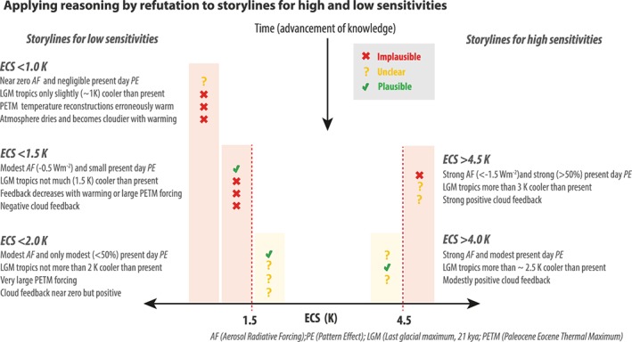
The application of refutational reasoning to storylines for successively more constraining bounds on ECS. For a particular bound on ECS to hold it must be consistent with all the lines of evidence, here formulated in terms of physical statements related to some interpretation of data or some specific process, for example, cloud response to warming. The hypotheses most fruitful to test progressively narrower bounds are those that are marked by a yellow question mark. This illustration is meant to encourage, rather than substitute, a more thorough assessment.

Condition (i) arises from the interpretation of the instrumental record using simple models whose value of the ECS is constrained by the data [e.g., Aldrin et al., 2012; Otto et al., 2013; Lewis and Curry, 2014]. These studies suggest that a value of the ECS less than 1.5 K would be consistent with changes in the energy budget and surface temperatures over the course of the instrumental record provided that the aerosol forcing and/or the historical “pattern effect”—which is neglected by the simple models—are modest (less than −1 W m⁻² and 50%, respectively). A weak to modest aerosol forcing is consistent with a broad range of evidence [Stevens, 2015] and although studies using comprehensive climate models suggest that the historical “pattern effect” is not negligible [Andrews, 2014; Huber et al., 2014], its magnitude is uncertain, making it difficult to refute condition (i).

Condition (ii) expresses the expectation that the temperature difference between the present and the LGM should increase with ECS. This expectation is not straightforward, because many details regarding the shape and height of great ice sheets at that time are poorly known, and uncertainties related to the response of the climate system to changing patterns of insolation confound predictions, particularly at middle and high latitudes [e.g., Braconnot et al., 2012; Jochum et al., 2012]. Aerosol forcing is also an uncertain factor. Nonetheless, model studies suggest that the decrease of tropical temperatures during the LGM offers some constraint on ECS [Schmittner et al., 2011; Hargreaves et al., 2012; Rohling et al., 2012; Schmidt et al., 2014]. This decrease, as evaluated on the basis of multiple proxies [Waelbroeck et al., 2009; Tripati et al., 2014; Annan and Hargreaves, 2015], appears too large to be reconciled with an ECS less than 1.5 K.

Going back further in the geological record one finds compelling evidence of very warm “hothouse” climates. Background temperatures in the early Eocene, during the Paleocene‐Eocene Thermal Maximum (about 56 Mya), and during more recent episodes appear to require climate sensitivities of 4–6 K, although the uncertainty in radiative forcing is considerable. To reconcile this with a modern ECS below 1.5 K requires either much higher greenhouse gas forcing than anticipated [Berner and Kothavala, 2001; Pagani et al., 2006; Alexander et al., 2015] or a weaker radiative response to warming at high global temperatures [Covey et al., 1996; Royer et al., 2007; Bijl et al., 2010; Rohling et al., 2012]. Models actually predict the latter to some extent [e.g., Meraner et al., 2013], but still have trouble simulating enough Eocene warmth unless the ECS is larger than about 3 K—hence condition (iii) also appears difficult to meet.

Finally we consider the implications of our understanding of the strength of feedbacks from specific physical processes on the value of the ECS. A very low ECS would either require a substantially negative cloud feedback or much weaker water vapor feedback than is freely simulated by any model [Sherwood et al., 2010]. In an attempt to force a model to achieve a weaker water vapor feedback, and a negative cloud feedback due to changes in high clouds [as suggested by Lindzen et al., 2001], low‐cloud cover also decreased, largely offsetting the intended effect [Mauritsen and Stevens, 2015]. A negative global cloud feedback is also very difficult to reconcile with understanding of cloud feedback mechanisms, which are overwhelmingly associated with positive feedbacks [see Appendix S1, also, Hartmann and Larson, 2002; Dessler, 2010; Zelinka and Hartmann, 2011; Webb and Lock, 2012; Boucher et al., 2013; Bretherton, 2015; Zhou et al., 2015; Bony et al., 2016]. An exception is a predicted negative cloud feedback at high latitudes where warming causes clouds to become more reflective [e.g., Betts and Harshvardhan, 1987; Zelinka et al., 2013; Kay et al., 2014]. Gordon and Klein [2014] provide evidence that this feedback is overestimated by models and even if not, it is outweighed by clouds becoming less reflective in middle and low latitudes. Observational tests of the feedback‐relevant processes in different models further identify the most realistic models as those having relatively strong positive feedback and high ECS [Clement et al., 2009; Sherwood et al., 2014; Su et al., 2014], nowhere near the net negative cloud feedback required for ECS <1.5 K.

5. Reasoning by Refutation and a Physical Storyline for a Very High ECS

Our physical storyline for a very high ECS (>4.5 K) is comprised of three conditions: (i) the aerosol cooling influence in recent decades would have to have been strong enough to offset most of the effect of rising greenhouse gases, or else the net radiative response to warming would have to have been at least twice as large for the last century as it will be in the future; (ii) tropical sea‐surface temperatures at the time of the LGM would have to have been much (3 K) cooler than at present; and (iii) cloud feedbacks from warming would have to be strong and positive.

Condition (i) arises from the relatively modest (near 1 K) warming seen in the instrumental record so far. The strong aerosol effect needed to reconcile a very high ECS with this warming is not consistent with values inferred from satellite data, and difficult to reconcile with the spatiotemporal structure of the instrumental record. Also aerosol effects on clouds saturate at high concentrations, which argues against a large effect [Boucher et al., 2013; Stevens, 2015]. There may, however, be other cooling mechanisms which blunted 20th‐century warming; for instance, the above‐mentioned “pattern effect” could have significantly damped 20th‐century warming compared to that which will occur over the longer term with the same forcing [Gregory and Andrews, 2016]. If so, this would reduce the magnitude of aerosol effect needed for this storyline to be true.

Condition (ii) likewise reflects similar reasoning as for the low‐ECS case. The LGM evidence is difficult to reconcile with a very high ECS, unless one allows for either a strong LGM “pattern effect” [cf. Hopcroft and Valdes, 2015] or feedbacks that grow more positive in warmer climates. There is in fact some support for each from climate models, which typically show both a pattern effect on cloud feedbacks [Senior and Mitchell, 2000; Armour et al., 2013; Geoffroy et al., 2013; Andrews et al., 2015; Knutti and Rugenstein, 2015] and an increase in the radiative forcing of successive CO₂ doublings [Gregory et al., 2015] and/or strengthening of cloud or water vapor feedbacks [Meraner et al., 2013], making this condition more plausible. Because evidence from “hothouse” climates seems unlikely to discount a very high ECS, the deep past does not play a role in this storyline.

Condition (iii) embodies understanding of physical processes, which imply that a very high ECS would require a strong positive feedback (>0.5 W m⁻²) from clouds. Attempts to assess the realism of such feedbacks are necessarily indirect. Strong cloud feedbacks do occur in some climate models, especially those models where cloud‐relevant processes better match observations [Clement et al., 2009; Sherwood et al., 2014; Su et al., 2014], consistent with understanding of important cloud controlling factors [Stevens and Brenguier, 2009; Rieck et al., 2012; Bretherton et al., 2013; Brient and Bony, 2013]. The strength of these feedbacks depends on the balance of sometimes opposing process [Zhang et al., 2013; Bretherton, 2015; Brient et al., 2015], and are sensitive to how the models are formulated [Gettelman et al., 2012; Qu et al., 2013; Zhao, 2014; Webb et al., 2015]. There is also some evidence that shallow‐cloud cover predicted by climate models may be oversensitive to local atmospheric properties [Nuijens et al., 2015], which could imply they exaggerate the amplitude of cloud feedbacks. These issues are discussed further in Appendix S1; until they are resolved, the evidence that understanding of cloud feedbacks are in conflict with the condition for the very high (ECS >4.5 K) storyline will remain weak, at best.

6. Combining the Different Lines of Evidence

In principle, refuting one of the conditions that must be satisfied for the ECS to exceed a given bound is sufficient to support the maintenance of that bound. A single red cross, the equivalent of a counter example in a mathematical proof, in Figure 1 is sufficient to falsify the hypothesis with which it is associated. In practice refutation is never this simple. To the extent a more nuanced, and quantitative, assessment of the confidence in a particular bound is desired, the rules of Bayesian inference provide a useful framework for combining different lines of evidence [Annan and Hargreaves, 2006; Hegerl et al., 2006; Annan, 2015].

For sake of argument, let χ denote the value of ECS, and S the evidence presented as a storyline. Bayesian inference calculates a posterior distribution as the probability of the hypothesis (in this case a value of χ) given the evidence. It is proportional to the likelihood of the evidence for a given value of χ times the prior distribution:

$$P\left(\chi |S\right)=\frac{P\left(S|\chi \right)P\left(\chi \right)}{P\left(S\right)}\text{.}$$ (1)

The likelihood of the storyline,

$$P\left(S\right)={\displaystyle {\int }_{-\infty }^{\infty }}P\left(S|\chi \right)P\left(\chi \right)\mathrm{d}\chi >0\text{,}$$ (2)

arises as a normalizing factor and ensures that the posterior integrates to unity. The probability that the ECS is within some bounds follows by integrating equation (1) over these bounds. The storyline is organized along its different conditions, which we associate with different lines of evidence. The conditions constituting a particular storyline were chosen on the basis of their differing evidentiary basis, and as such are treated as being independent.

To illustrate the method we consider the storylines for a very low, <1.5 K, and very high, >4.5 K, ECS. Let us denote evidence related to the jth condition for the storyline S by e _j. The assumed independence of N different lines of evidence yields:

$$P\left(S|\chi \right)={\displaystyle \prod _{j=1}^N}P\left(e_j|\chi \right)\text{.}$$ (3)

Reasoning by refutation is akin to saying that the probability of the evidence is low if the hypothesis is false but high if it is true. We model this by specifying each P(e _j|χ) as a function that transitions from a likelihood α _j to 1 − α _j following an error function centered at some critical ECS, χ _j, near the hypothesized bound (see Figure 2a and Appendix S1). The α _j thus express the likelihood that the evidence, which appears to refute a particular hypothesis, is misleading. A smaller value of α _j expressing more confidence that the evidence refutes the hypothesis. The form of the likelihood function we have adopted requires α _j ≤ 0.5 and thereby ensures that only storylines are considered whose refutation is more likely than not.

Figure 2.

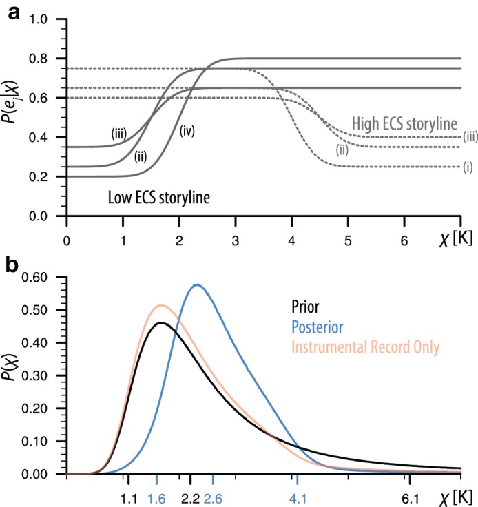
(a) Likelihoods of evidence refuting a particular storyline of being misleading given a value of the ECS (denoted by χ) and differentiated by the storyline conditions for a very low ECS (solid) and very high ECS (dashed); (b) the prior (black) and posterior (blue) distributions with 5, 50, and 95 percentiles of the respective distributions indicated by major tick marks. The case when only one line of evidence is considered, here the instrumental record (coral colored line), unduly emphasizes those values of ECS which it does not constrain.

The α _j and the χ _j are determined by the nature of the evidence. For the very low ECS storyline, we have some confidence that conditions (ii)–(iv) contraindicate the hypothesis (cf. discussion above, Figures 1 and S1). Hence for these conditions we adopt a likelihood α _j of 0.25, 0.35, 0.20, respectively, with χ _j = 1.5 K for conditions (ii) and (iii), and χ _j = 2 K for condition (iv). Likewise we have some confidence that conditions (i)–(iii) contraindicate the hypothesis of a very high ECS and for these we adopt a likelihood α _j of 0.25, 0.35, 0.40, respectively, with χ _j = 4.5 K for conditions (ii) and (iii), and χ _j = 4 K for condition (i). All six conditions (Figure 2a) have been constructed from a reasonable consideration of the evidence (as discussed in the Appendix S1), but also with our didactic purpose in mind.

As the prior distribution should be based on knowledge independent of the evidence subsequently applied to the range of ECS, we chose a prior that arises from our most robust and basic understanding of atmospheric physics [Stevens and Bony, 2013; Zelinka et al., 2016, and Appendix S1]. We thus choose as the prior an ECS composed by forming the ratio of an effective radiative forcing and a feedback parameter, with a 20% (1‐sigma) width Gaussian distribution in the effective forcing and a 50% width Gaussian in the feedback parameter λ with the resultant distribution bounded (truncated and normalized) between 0 and 10 K. This choice of prior (Figure 2b) yields a 19% chance that ECS <1.5 K and a 11% chance that ECS >4.5 K (Figure 2b). Combining this prior with the different lines of evidence following equation (1) results in a narrower posterior distribution, one with only a 3% chance of ECS being <1.5 K, and a similarly small chance of ECS being >4.5 K. The posteriori estimate is relatively insensitive to modest changes in the prior, or how we assess the evidence that appears to refute the storyline for a high ECS (Appendix S1). This is less true if only a single line of evidence in isolation is considered, as reasoning from a single line of evidence is more prone to be misleading. For instance, taking only the instrumental record, which appears to rule out a very high ECS, actually ends up increasing the chance of ECS <1.5 K (Figure 2b).

We nonetheless caution against focusing too narrowly on the posterior distribution that emerges from one or the other example. As doing so risks missing the point, which is to illustrate the role of different lines of evidence in modifying a prior judgment. In evaluating how different physical storylines shape thinking as to which values of ECS seem implausible it will be important to argue about the choice of the prior, the likelihoods assigned to different lines of evidence, and their degree of independence. In this spirit, our examples help demonstrate how a physical storyline can help to quantify confidence in a particular ECS bound and make transparent the role of different lines of evidence.

7. Prospects for Narrowing Uncertainty

By elucidating the reasoning behind a given bound on ECS, the storyline approach helps define research directions that could refine and narrow the ECS range. For instance, greater confidence in the sign of cloud feedbacks would have implications for the lower bound on ECS. We estimate that increased confidence in a net positive cloud feedback may be sufficient to refute a condition of the storyline for an ECS less than 2.0 K (see Appendix S1). Better reconstructions of the tropical temperatures at the time of the LGM, or greenhouse gas levels in past “hothouse” climates, could also lift this lower bound.

Critical tests for the upperbound could be provided by a better understanding of pattern effects, or by testing recent arguments for a more modest aerosol forcing [Stevens, 2015]. They could also come from glacial cycle evidence, either via better understanding of pattern effects or improved proxy evidence—especially temperature reconstructions. Importantly, a more specific understanding of low‐cloud feedback mechanisms [e.g., Sherwood et al., 2014] now makes it possible to design field experiments in ways that can better address cloud feedback mechanisms. Such field studies, together with high‐resolution modeling, may offer the best opportunity to refine the upper bound of ECS by ruling out very strong positive cloud feedbacks.

Attempts to tighten the bounds on ECS may also need to account for recent findings that the radiative forcing from rising greenhouse gases is less tightly constrained by ab initio calculations than is commonly thought [e.g., Geoffroy et al., 2013; Vial et al., 2013]. Recent work makes a compelling case that the radiative impact of a change in the atmosphere's composition can be modified by poorly understood changes in cloudiness (or surface reflectance) that arise in response to a perturbing agent in the absence of global surface warming [Gregory and Webb, 2008; Sherwood et al., 2015]. Present evidence does not suggest that this is a large effect, but the uncertainty it introduces into forcing estimates will become more important as uncertainty in ECS is reduced.

8. Refutational Reasoning: Linking Assessments to Storylines

Explicitly laying out the storylines for exceeding a particular ECS bound achieves two important things. First, it illustrates the constraining power of different lines of evidence; refutational reasoning then reveals why experts broadly familiar with this evidence are so skeptical about very high or very low ECS values, even though individual lines of evidence considered in isolation would not merit such skepticism and may sometimes even support such values. Second, it clarifies what evidence is most important, and from where improvements in our knowledge of the ECS are most likely to come. As Bony et al. [2015] argued in a different context, physical storylines thus support a more active and effective assessment process, one in which important gaps in understanding—and the strategies needed to fill them—are naturally identified. The physical storylines explored here are powerful, but how absolute or definitive they are, and whether our approach for combining different lines of evidence is as promising as it appears, remains to be judged. A formal and thorough assessment is needed.

Erratum

The bounds on the prior were clarified by the authors after the publication of this article. The article and its supporting information have been updated, and this may be considered the official version of record.

Supporting information

Supporting Information S1

References

- Aldrin, M. , Holden M., Guttorp P., Skeie R. B., Myhre G., and Berntsen T. K. (2012), Bayesian estimation of climate sensitivity based on a simple climate model fitted to observations of hemispheric temperatures and global ocean heat content, Environmetrics, 23(3), 253–271, doi: 10.1002/env.2140. [DOI] [Google Scholar]
- Alexander, K. , Meissner K. J., and Bralower T. J. (2015), Sudden spreading of corrosive bottom water during the Palaeocene‐Eocene Thermal Maximum, Nat. Geosci., 8(6), 458–461, doi: 10.1038/ngeo2430. [DOI] [Google Scholar]
- Allen, M. R. , and Frame D. J. (2007), Call off the quest, Science, 318(5850), 582–583, doi: 10.1126/science.1149988. [DOI] [PubMed] [Google Scholar]
- Andrews, T. (2014), Using an AGCM to diagnose historical effective radiative forcing and mechanisms of recent decadal climate change, J. Clim., 27(3), 1193–1209, doi: 10.1175/JCLI-D-13-00336.1. [DOI] [Google Scholar]
- Andrews, T. , Gregory J. M., and Webb M. J. (2015), The dependence of radiative forcing and feedback on evolving patterns of surface temperature change in climate models, J. Clim., 28(4), 1630–1648, doi: 10.1175/JCLI-D-14-00545.1. [DOI] [Google Scholar]
- Annan, J. D. (2015), Recent developments in Bayesian estimation of climate sensitivity, Curr. Clim. Change Rep., 1(4), 263–267, doi: 10.1007/s40641-015-0023-5. [DOI] [Google Scholar]
- Annan, J. D. , and Hargreaves J. C. (2006), Using multiple observationally‐based constraints to estimate climate sensitivity, Geophys. Res. Lett., 33, L06704, doi: 10.1029/2005GL025259. [DOI] [Google Scholar]
- Annan, J. D. , and Hargreaves J. C. (2015), A perspective on model‐data surface temperature comparison at the Last Glacial Maximum, Quat. Sci. Rev., 107, 1–10, doi: 10.1016/j.quascirev.2014.09.019. [DOI] [Google Scholar]
- Armour, K. C. , Bitz C. M., and Roe G. H. (2013), Time‐varying climate sensitivity from regional feedbacks, J. Clim., 26(13), 4518–4534, doi: 10.1175/JCLI-D-12-00544.1. [DOI] [Google Scholar]
- Arrhenius, S. (1896), On the influence of carbonic acid in the air upon the temperature of the ground, Philos. Mag. Ser. , 41(251), 237–276, doi: 10.1080/14786449608620846. [DOI] [Google Scholar]
- Berner, R. A. , and Kothavala Z. (2001), Geocarb III: A revised model of atmospheric CO2 over Phanerozoic time, Am. J. Sci., 301(2), 182–204, doi: 10.2475/ajs.301.2.182. [DOI] [Google Scholar]
- Betts, A. K. , and Harshvardhan (1987), Thermodynamic constraint on the cloud liquid water feedback in climate models, J. Geophys. Res. Atmos., 92(D7), 8483–8485, doi: 10.1029/JD092iD07p08483. [DOI] [Google Scholar]
- Bijl, P. K. , Houben A. J. P., Schouten S., Bohaty S. M., Sluijs A., Reichart G.‐J., Damste J. S. S., and Brinkhuis H. (2010), Transient middle eocene atmospheric CO2 and temperature variations, Science, 330(6005), 819–821, doi: 10.1126/science.1193654. [DOI] [PubMed] [Google Scholar]
- Bony, S. , Stevens B., Held I. H., Mitchell J. F., Dufresne J.‐L., Emanuel K. A., Friedlingstein P., Griffies S., and Senior C. (2013), Carbon dioxide and climate: Perspectives on a scientific assessment, in Climate Science for Serving Society, edited by Hurrell J. W. and Asrar G., pp. 391–413 , Springer Netherlands, Dordrecht, the Netherlands. [Google Scholar]
- Bony, S. , et al. (2015), Clouds, circulation and climate sensitivity, Nat. Geosci., 8(4), 261–268, doi: 10.1038/ngeo2398. [DOI] [Google Scholar]
- Bony, S. , Stevens B., Coppin D., Becker T., Reed K. A., Voigt A., and Medeiros B. (2016), Thermodynamic control of anvil cloud amount, Proc. Natl. Acad. Sci. U. S. A., 113(32), 8927–8932. [DOI] [PMC free article] [PubMed] [Google Scholar]
- Boucher, O. , et al. (2013), Clouds and aerosols, in Climate Change 2013: The Physical Science Basis. Contribution of Working Group I to the Fifth Assessment Report of the Intergovernmental Panel on Climate Change, edited by Stocker T. F., Qin D., Plattner G. K., Tignor M., Allen S. K., Boschung J., Nauels A., Xia Y., Bex V., and Midgley P. M., pp. 571–657 , Cambridge Univ. Press, Cambridge, UK and New York. [Google Scholar]
- Braconnot, P. , Harrison S. P., Kageyama M., Bartlein P. J., Masson‐Delmotte V., Abe‐Ouchi A., Otto‐Bliesner B., and Zhao Y. (2012), Evaluation of climate models using palaeoclimatic data, Nat. Clim. Change, 2(6), 417–424, doi: 10.1038/nclimate1456. [DOI] [Google Scholar]
- Bretherton, C. S. (2015), Insights into low‐latitude cloud feedbacks from high‐resolution models, Philos. Trans. R. Soc. A, 373(2054), 20140415, doi: 10.1098/rsta.2014.0415. [DOI] [PubMed] [Google Scholar]
- Bretherton, C. S. , Blossey P. N., and Jones C. R. (2013), Mechanisms of marine low cloud sensitivity to idealized climate perturbations: A single‐LES exploration extending the CGILS cases, J. Adv. Model. Earth Syst., 5(2), 316–337, doi: 10.1002/JAME.20019. [DOI] [Google Scholar]
- Brient, F. , and Bony S. (2013), Interpretation of the positive low‐cloud feedback predicted by a climate model under global warming, Clim. Dyn., 40(9–10), 2415–2431, doi: 10.1007/s00382-011-1279-7. [DOI] [Google Scholar]
- Brient, F. , Schneider T., Tan Z., Bony S., Qu X., and Hall A. (2015), Shallowness of tropical low clouds as a predictor of climate models' response to warming, Clim. Dyn., 47(1–2), 433–449. [Google Scholar]
- Charney, J. G. , Arakawa A., Baker D. J., Bolin B., Dickinson R. E., Goody R. M. , Leith C. E., Stommel H. M., and Wunsch C. I. (1979), Carbon dioxide and climate: A scientific assessment, National Academy of Sciences, Washington, D. C.
- Clement, A. C. , Burgman R., and Norris J. R. (2009), Observational and model evidence for positive low‐level cloud feedback, Science, 325(5939), 460–464, doi: 10.1126/science.1171255. [DOI] [PubMed] [Google Scholar]
- Collins, M. , et al. (2013), Long‐term climate change: Projections, commitments and irreversibility, in Climate Change 2013: The Physical Science Basis. Contribution of Working Group I to the Fifth Assessment Report of the Intergovernmental Panel on Climate Change, edited by Stocker T. F., Qin D., Plattner G. K., Tignor M., Allen S. K., Boschung J., Nauels A., Xia Y., Bex V., and Midgley P. M., pp. 1029–1136 , Cambridge Univ. Press, Cambridge, UK and New York. [Google Scholar]
- Cooke, R. , Wielicki B. A., Young D. F., and Mlynczak M. G. (2013), Value of information for climate observing systems, Environ. Syst. Decis., 34(1), 98–109, doi: 10.1007/s10669-013-9451-8. [DOI] [Google Scholar]
- Covey, C. , Sloan L. C., and Hoffert M. I. (1996), Paleoclimate data constraints on climate sensitivity: The paleocalibration method, Clim. Change, 32(2), 165–184, doi: 10.1007/BF00143708. [DOI] [Google Scholar]
- Dessler, A. E. (2010), A determination of the cloud feedback from climate variations over the past decade, Science, 330(6010), 1523–1527, doi: 10.1126/science.1192546. [DOI] [PubMed] [Google Scholar]
- Dessler, A. E. (2013), Observations of climate feedbacks over 2000–10 and comparisons to climate models, J. Clim., 26(1), 333–342, doi: 10.1175/JCLI-D-11-00640.1. [DOI] [Google Scholar]
- Dufresne, J.‐L. , and Saint‐Lu M. (2016), Positive feedback in climate: Stabilization or runaway, illustrated by a simple experiment, Bull. Am. Meteorol. Soc., 97(2), 755–765, doi: 10.1175/BAMS-D-14-00022.1. [DOI] [Google Scholar]
- Flato, G. , et al. (2013), Evaluation of climate models, in Climate Change 2013: The Physical Science Basis. Contribution of Working Group I to the Fifth Assessment Report of the Intergovernmental Panel on Climate Change, edited by Stocker T. F., Qin D., Plattner G. K., Tingor M., Allen S. K., Boschung J., Nauels A., Xia Y., Bex V., and Midgley P. M., pp. 741–866 , Cambridge Univ. Press, Cambridge, UK and New York. [Google Scholar]
- Forster, P. M. (2016), Inference of climate sensitivity from analysis of earth's energy budget, Annu. Rev. Earth Planet. Sci., 44(1), 85–106, doi: 10.1146/annurev-earth-060614-105156. [DOI] [Google Scholar]
- Geoffroy, O. , Saint‐Martin D., Olivié D. J. L., Voldoire A., Bellon G., and Tyteca S. (2013), Transient climate response in a two‐layer energy‐balance model. Part I: Analytical solution and parameter calibration using CMIP5 AOGCM experiments, J. Clim., 26(6), 1841–1857, doi: 10.1175/JCLI-D-12-00195.1. [DOI] [Google Scholar]
- Gettelman, A. , Kay J. E., and Shell K. M. (2012), The evolution of climate sensitivity and climate feedbacks in the community atmosphere model, J. Clim., 25(5), 1453–1469, doi: 10.1175/JCLI-D-11-00197.1. [DOI] [Google Scholar]
- Gordon, N. D. , and Klein S. A. (2014), Low‐cloud optical depth feedback in climate models, J. Geophys. Res. Atmos., 119(10), 6052–6065, doi: 10.1002/2013JD021052. [DOI] [Google Scholar]
- Gregory, J. , and Webb M. (2008), Tropospheric adjustment induces a cloud component in CO2 forcing, J. Clim., 21(1), 58–71, doi: 10.1175/2007JCLI1834.1. [DOI] [Google Scholar]
- Gregory, J. M. , Andrews T., and Good P. (2015), The inconstancy of the transient climate response parameter under increasing CO2 , Philos. Trans. R. Soc. A, 373(2054), 1–25. [DOI] [PMC free article] [PubMed] [Google Scholar]
- Gregory, J. M. , and Andrews T. (2016), Variation in climate sensitivity and feedback parametersduring the historical period, Geophys. Res. Lett., 43, 3911–3920, doi: 10.1002/2016GL068406. [DOI] [Google Scholar]
- Hargreaves, J. C. , Annan J. D., Yoshimori M., and Abe‐Ouchi A. (2012), Can the last glacial maximum constrain climate sensitivity? Geophys. Res. Lett., 39(24), L24702. [Google Scholar]
- Hartmann, D. L. , and Larson K. (2002), An important constraint on tropical cloud – climate feedback, Geophys. Res. Lett., 29(20), 1951, doi: 10.1029/2002GL015835. [DOI] [Google Scholar]
- Hegerl, G. C. , Crowley T. J., Hyde W. T., and Frame D. J. (2006), Climate sensitivity constrained by temperature reconstructions over the past seven centuries, Nature, 440, 1029–1032, doi: 10.1038/nature04679. [DOI] [PubMed] [Google Scholar]
- Held, I. M. , Winton M., Takahashi K., Delworth T., Zeng F., and Vallis G. K. (2010), Probing the fast and slow components of global warming by returning abruptly to preindustrial forcing, J. Clim., 23(9), 2418–2427, doi: 10.1175/2009JCLI3466.1. [DOI] [Google Scholar]
- Hopcroft, P. O. , and Valdes P. J. (2015), How well do simulated last glacial maximum tropical temperatures constrain equilibrium climate sensitivity? Geophys. Res. Lett., 42(13), 5533–5539, doi: 10.1002/2015GL064903. [DOI] [Google Scholar]
- Huber, M. , Beyerle U., and Knutti R. (2014), Estimating climate sensitivity and future temperature in the presence of natural climate variability, Geophys. Res. Lett., 41(6), 2086–2092, doi: 10.1002/2013GL058532. [DOI] [Google Scholar]
- Jochum, M. , Jahn A., Peacock S., Bailey D. A., Fasullo J. T., Kay J., Levis S., and Otto‐Bliesner B. (2012), True to Milankovitch: Glacial inception in the new community climate system model, J. Clim., 25(7), 2226–2239, doi: 10.1175/JCLI-D-11-00044.1. [DOI] [Google Scholar]
- Kang, S. M. , Held I. M., and Xie S.‐P. (2013), Contrasting the tropical responses to zonally asymmetric extratropical and tropical thermal forcing, Clim. Dyn., 42(7–8), 2033–2043. [Google Scholar]
- Kay, J. E. , Medeiros B., Hwang Y. T., Gettelman A., Perket J., and Flanner M. G. (2014), Processes controlling Southern Ocean shortwave climate feedbacks in CESM, Geophys. Res. Lett., 41(2), 616–622, doi: 10.1002/2013GL058315. [DOI] [Google Scholar]
- Knutti, R. , and Hegerl G. C. (2008), The equilibrium sensitivity of the Earth's temperature to radiation changes, Nat. Geosci., 1(11), 735–743, doi: 10.1038/ngeo337. [DOI] [Google Scholar]
- Knutti, R. , and Rugenstein M. A. A. (2015), Feedbacks, climate sensitivity and the limits of linear models, Philos. Trans. R. Soc. A, 373(2054), 20150146, doi: 10.1098/rsta.2015.0146. [DOI] [PubMed] [Google Scholar]
- Kuang, Z. , and Hartmann D. L. (2007), Testing the fixed anvil temperature hypothesis in a cloud‐resolving model, J. Clim., 20(10), 2051–2057, doi: 10.1175/JCLI4124.1. [DOI] [Google Scholar]
- Lewis, N. , and Curry J. A. (2014), The implications for climate sensitivity of AR5 forcing and heat uptake estimates, Clim. Dyn., 45, 1009–1023. [Google Scholar]
- Li, C. , Storch J.‐S., and Marotzke J. (2012), Deep‐ocean heat uptake and equilibrium climate response, Clim. Dyn., 41, 1071–1086. [Google Scholar]
- Lindzen, R. , Chou M. D., and Hou A. Y. (2001), Does the earth have an adaptive infrared iris? Bull. Am. Meteorol. Soc., 83(2), 417–432, doi:. [DOI] [Google Scholar]
- Loeb, N. G. , Wielicki B. A., Doelling D. R., Smith G. L., Keyes D. F., Kato S., Manalo‐Smith N., and Wong T. (2009), Toward optimal closure of the Earth's top‐of‐atmosphere radiation budget, J. Clim., 22(3), 748–766, doi: 10.1175/2008JCLI2637.1. [DOI] [Google Scholar]
- Lüthi, D. , et al. (2008), High‐resolution carbon dioxide concentration record 650,000–800,000 years before present, Nature, 453(7193), 379–382, doi: 10.1038/nature06949. [DOI] [PubMed] [Google Scholar]
- MacDougall, A. H. (2016), The transient response to cumulative CO2 emissions: A review, Curr. Clim. Change Rep., 2(1), 39–47, doi: 10.1007/s40641-015-0030-6. [DOI] [Google Scholar]
- Mauritsen, T. , and Stevens B. (2015), Missing iris effect as a possible cause of muted hydrological change and high climate sensitivity in models, Nat. Geosci., 8, 346–351. [Google Scholar]
- Meraner, K. , Mauritsen T., and Voigt A. (2013), Robust increase in equilibrium climate sensitivity under global warming, Geophys. Res. Lett., 40(22), 5944–5948, doi: 10.1002/2013GL058118. [DOI] [Google Scholar]
- Morice, C. P. , Kennedy J. J., Rayner N. A., and Jones P. D. (2012), Quantifying uncertainties in global and regional temperature change using an ensemble of observational estimates: The HadCRUT4 data set, J. Geophys. Res. Atmos., 117(D8), D08101. [Google Scholar]
- Neubersch, D. , Held H., and Otto A. (2014), Operationalizing climate targets under learning: An application of cost‐risk analysis, Clim. Change, 126(3–4), 305–318, doi: 10.1007/s10584-014-1223-z. [DOI] [Google Scholar]
- Nuijens, L. , Medeiros B., Sandu I., and Ahlgrimm M. (2015), The behavior of trade‐wind cloudiness in observations and models: The major cloud components and their variability, J. Adv. Model. Earth Syst., 7(2), 600–616, doi: 10.1002/2014MS000390. [DOI] [Google Scholar]
- Otto, A. , et al. (2013), Energy budget constraints on climate response, Nat. Geosci., 6, 415–416, doi: 10.1038/ngeo1836. [DOI] [Google Scholar]
- Pagani, M. , Caldeira K., Archer D., and Zachos J. C. (2006), An ancient carbon mystery, Science, 314(5805), 1556–1557, doi: 10.1126/science.1136110. [DOI] [PubMed] [Google Scholar]
- Pagani, M. , Huber M., Sageman B. (2014), Greenhouse Climates, In Treatise on Geochemistry (Second Edition), edited by Holland H.D. and Turekian K.K., Elsevier, Oxford, 281–304, doi: 10.1016/B978-0-08-095975-7.01314-0. [DOI] [Google Scholar]
- Pierrehumbert, R. T. , Abbot D. S., Voigt A., and Koll D. (2011), Climate of the neoproterozoic, Annu. Rev. Earth Planet. Sci., 39(1), 417–460, doi: 10.1146/annurev-earth-040809-152447. [DOI] [Google Scholar]
- Qu, X. , Hall A., Klein S. A., and Caldwell P. M. (2013), On the spread of changes in marine low cloud cover in climate model simulations of the 21st century, Clim. Dyn., 42(9–10), 2603–2626. [Google Scholar]
- Rieck, M. , Nuijens L., and Stevens B. (2012), Marine boundary layer cloud feedbacks in a constant relative humidity atmosphere, J. Atmos. Sci., 69(8), 2538–2550, doi: 10.1175/JAS-D-11-0203.1. [DOI] [Google Scholar]
- Rohling, E. J. , et al. (2012), Making sense of palaeoclimate sensitivity, Nature, 491(7426), 683–691, doi: 10.1038/nature11574. [DOI] [PubMed] [Google Scholar]
- Royer, D. L. , Berner R. A., and Park J. (2007), Climate sensitivity constrained by CO2 concentrations from the last 420 million years, Nature, 446, 530–532, doi: 10.1038/nature05699. [DOI] [PubMed] [Google Scholar]
- Schmidt, G. A. , et al. (2014), Using palaeo‐climate comparisons to constrain future projections in CMIP5, Clim. Past, 10(1), 221–250, doi: 10.5194/cp-10-221-2014. [DOI] [Google Scholar]
- Schmittner, A. , Urban N. M., Shakun J. D., Mahowald N. M., Clark P. U., Bartlein P. J., Mix A. C., and Rosell‐Mele A. (2011), Climate sensitivity estimated from temperature reconstructions of the last glacial maximum, Science, 334(6061), 1385–1388, doi: 10.1126/science.1203513. [DOI] [PubMed] [Google Scholar]
- Seneviratne, S. I. , Donat M. G., Pitman A. J., Knutti R., and Wilby R. L. (2016), Allowable CO2 emissions based on regional and impact‐related climate targets, Nature, 529(7587), 477–483, doi: 10.1038/nature16542. [DOI] [PubMed] [Google Scholar]
- Senior, C. A. , and Mitchell J. F. B. (2000), The time‐dependence of climate sensitivity, Geophys. Res. Lett., 27(17), 2685–2688, doi: 10.1029/2000GL011373. [DOI] [Google Scholar]
- Sherwood, S. C. , Ingram W., Tsushima Y., Satoh M., Roberts M., Vidale P. L., and O'Gorman P. A. (2010), Relative humidity changes in a warmer climate, J. Geophys. Res. Atmos., 115(D9), D09104, doi: 10.1029/2009JD012585. [DOI] [Google Scholar]
- Sherwood, S. C. , Bony S., and Dufresne J.‐L. (2014), Spread in model climate sensitivity traced to atmospheric convective mixing, Nature, 505(7481), 37–42, doi: 10.1038/nature12829. [DOI] [PubMed] [Google Scholar]
- Sherwood, S. C. , Bony S., Boucher O., Bretherton C., Forster P. M., Gregory J. M., and Stevens B. (2015), Adjustments in the forcing‐feedback framework for understanding climate change, Bull. Am. Meteorol. Soc., 96(2), 217–228, doi: 10.1175/BAMS-D-13-00167.1. [DOI] [Google Scholar]
- Stevens, B. (2015), Rethinking the lower bound on aerosol radiative forcing, J. Clim., 28(12), 4794–4819, doi: 10.1175/JCLI-D-14-00656.1. [DOI] [Google Scholar]
- Stevens, B. , and Bony S. (2013), Water in the atmosphere, Phys. Today, 66(6), 29, doi: 10.1063/PT.3.2009. [DOI] [Google Scholar]
- Stevens, B. , and Brenguier J.‐L. (2009), Cloud‐controlling factors: Low clouds, in Clouds in the Perturbed Climate System, edited by Heintzenberg J. and Charlson R. J., pp. 1–24 , MIT Press, Cambridge, Mass.. [Google Scholar]
- Stevens, B. , Abe‐Ouchi A., Bony S., Hegerl G. C., Schmidt G. A., Sherwood S. C., and Webb M. J. (2015), Ringberg15: Earth's climate sensitivities, Tech. Rep. 11, World Climate Research Programme, Geneva, Switzerland.
- Stocker, T. F. , Qin D., Plattner G. K., Tingor M., Allen S. K., Boschung J., Nauels A., Xia Y., Bex V., and Midgley P. M. (2013), IPCC, 2013, Climate Change 2013: The Physical Science Basis. Contribution of Working Group I to the Fifth Assessment Report of the Intergovernmental Panel on Climate Change, vol. 413, Cambridge Univ. Press, Berlin and Heidelberg. [Google Scholar]
- Su, H. , Jiang J. H., Zhai C., Shen T. J., Neelin J. D., Stephens G. L., and Yung Y. L. (2014), Weakening and strengthening structures in the Hadley Circulation change under global warming and implications for cloud response and climate sensitivity, J. Geophys. Res. Atmos., 119(10), 5787–5805, doi: 10.1002/2014JD021642. [DOI] [Google Scholar]
- Tebaldi, C. , and Arblaster J. M. (2014), Pattern scaling: Its strengths and limitations, and an update on the latest model simulations, Clim. Change, 122(3), 459–471, doi: 10.1007/s10584-013-1032-9. [DOI] [Google Scholar]
- Tripati, A. K. , Sahany S., Pittman D., Eagle R. A., Neelin J. D., Mitchell J. L., and Beaufort L. (2014), Modern and glacial tropical snowlines controlled by sea surface temperature and atmospheric mixing, Nat. Geosci., 7(3), 205–209, doi: 10.1038/ngeo2082. [DOI] [Google Scholar]
- Vial, J. , Dufresne J.‐L., and Bony S. (2013), On the interpretation of inter‐model spread in CMIP5 climate sensitivity estimates, Clim. Dyn., 41(11–12), 3339–3362, doi: 10.1007/s00382-013-1725-9. [DOI] [Google Scholar]
- Waelbroeck, C. , et al. (2009), Constraints on the magnitude and patterns of ocean cooling at the Last Glacial Maximum, Nat. Geosci., 2(2), 127–132, doi: 10.1038/ngeo411. [DOI] [Google Scholar]
- Webb, M. J. , and Lock A. P. (2012), Coupling between subtropical cloud feedback and the local hydrological cycle in a climate model, Clim. Dyn., 41(7–8), 1923–1939. [Google Scholar]
- Webb, M. J. , et al. (2015), The impact of parametrized convection on cloud feedback, Philos. Trans. R. Soc. A, 373(2054), 20140414, doi: 10.1098/rsta.2014.0414. [DOI] [PMC free article] [PubMed] [Google Scholar]
- Winton, M. , Takahashi K., and Held I. M. (2010), Importance of ocean heat uptake efficacy to transient climate change, J. Clim., 23(9), 2333–2344, doi: 10.1175/2009JCLI3139.1. [DOI] [Google Scholar]
- Zelinka, M. D. , and Hartmann D. L. (2011), The observed sensitivity of high clouds to mean surface temperature anomalies in the tropics, J. Geophys. Res. Atmos., 116(D23), D23103, doi: 10.1029/2011JD016459. [DOI] [Google Scholar]
- Zelinka, M. D. , Klein S. A., Taylor K. E., Andrews T., Webb M. J., Gregory J. M., and Forster P. M. (2013), Contributions of different cloud types to feedbacks and rapid adjustments in CMIP5*, J. Clim., 26(14), 5007–5027, doi: 10.1175/JCLI-D-12-00555.1. [DOI] [Google Scholar]
- Zelinka, M. D. , Zhou C., and Klein S. A. (2016), Insights from a refined decomposition of cloud feedbacks, Geophys. Res. Lett., 43, 9259–9269, doi: 10.1002/2016GL069917. [DOI] [Google Scholar]
- Zhang, M. , et al. (2013), CGILS: Results from the first phase of an international project to understand the physical mechanisms of low cloud feedbacks in single column models, J. Adv. Model. Earth Syst., 5(4), 826–842, doi: 10.1002/2013MS000246. [DOI] [Google Scholar]
- Zhao, M. (2014), An Investigation of the connections among convection, clouds, and climate sensitivity in a global climate model, J. Clim., 27(5), 1845–1862, doi: 10.1175/JCLI-D-13-00145.1. [DOI] [Google Scholar]
- Zhou, C. , Zelinka M. D., and Dessler A. E. (2015), The relationship between interannual and long‐term cloud feedbacks, Geophys. Res. Lett., 42, 10,463–10,469, doi: 10.1002/2015GL066698. [DOI] [Google Scholar]
Associated Data
This section collects any data citations, data availability statements, or supplementary materials included in this article.
Supplementary Materials