Abstract
Background
Previous studies present various methods for prediction disease based on statistics or neural networks.These models use statistics and results from past procedures to provide prediction through probability analysis.
Objective
In this article, the authors present a dynamic model aiming at predicting the treatment result of infertile women with the factor of polycystic ovary syndrome.
Materials and Methods
For this purpose, the authors have divided the study population into five groups: women prone to infertility, PCOS women, infertile women undergoing the treatment with Clomiphene Citrate and Gonadotropin, infertile women under IVF treatment, and improved infertile women. Therefore, the authors modeled the disease in infertile women mathematically and indicated that the free equilibrium point was asymptotically stable. Also the possibility of other equilibrium point of the system has been studied.
Results
The authors showed that this equilibrium point was marginally stable. Using Stoke's Theorem, the authors proved that the recurrence of the disease cycle with the factor of polycystic ovary syndrome was not intermittent in infertile women. They solved this model numerically using Rung-Kutta method and sketched the figures of the resulted solutions.
Conclusion
It shows that with increasing age, the ovarian reserve is decreased and the treatment Clomiphene Citrate and Gonadotropin are not responsive, so IVF treatment is recommended in this group of patients considering the graphs of the model.
Keywords: Infertility, Polycystic ovary syndrome, In vitro fertilization, Asymptotically stable, Differential equation, Free equilibrium point
1. Introduction
Infertility is referred to the inability of a woman to become pregnant after at least one year of regular sexual intercourse without using birth control. Infertility is seen in 10–15% of couples (1). The main causes of infertility include: ovulatory dysfunction, tuboperitoneal pathology, male factors, and uterine pathology (2). One of the most common causes of ovulatory dysfunction is the polycystic ovary syndrome. In 2003 Rotterdam, the presence of two out of three criteria for diagnosis of PCOS is essential. (i) Clinical and/or biochemical signs of hyperandrogenism, (ii) Oligomenorrhea or anovulation, and (iii) polycystic ovaries (with the exclusion of related disorders) (3). In most cases, women with PCOS have reduced fertility due to low ovulation; therefore, the ovarian stimulation methods are used for a group of these patients due to their reduced ovarian response. Clomiphene Citrate is the major component of the ovarian stimulation treatment, causing 80–85% of the ovulation and leading to pregnancy in 40% of women (2) Gynecologists suggest that after a maximum of six months being in ovulation cycles with the use of Clomiphene Citrate, it is better for the patient to be treated with gonadotrophin. If the treatment cycles with Clomiphene Citrate and Gonadotropin are determined and its therapeutic follow-up is controlled, and yet the pregnancy does not occur during the 9-12 treatment cycles, the ovulation stimulation method should not be relied upon. Therefore, using the Assisted Reproductive Techniques (ART), one of which is IVF, is recommended. Here, we present a model for women infertility with polycystic ovary syndrome, based on the individuals who went to the Yazd Infertility Research and Treatment Clinic. To this end, we show the total number of the infertile couples who at the time of t went to the clinic over the course of a year, with N(t). We have divided them into five groups, including: the newcomers who went to the clinic and their disease has not yet been confirmed, patients (those whose disease has been diagnosed to be and should be treated by this clinic), those treated with Clomiphene Citrate and Gonadotropin, those treated with ART, and improved patients (those whose test was positive). We call this our model.
In the second section, we model infertility in women with PCOS using dynamic system methods and find the number of the secondary sufferers during the course of the disease that had returned to the disease, and we show it with .
In the third section, we obtain the equilibrium point of the model , using geometric methods and examine its stability, asymptotically.
In the fourth section, we examine the stability of the disease asymptotically in the equilibrium point.
In the fifth section, using the Stoke's Theorem, we examine the non-intermittence of the therapeutic cycle.
In the sixth section, the model is solved numerically by using Rung-Kutta method, and the obtained data are summarized in the several graphs, which are analyzed in detail.
2. Materials and Methods
According to the previous section, we show the total number of the infertile women at time with . Therefore, .
Suppose and refer to the birth rate of the disease (the rate of the patient's arrival at the clinic to diagnose and treat their disease) and the death rate (leaving the clinic without any result or not being treated), respectively. By `not being treated', we mean those who were checked at the clinic, and the type of their treatment was diagnosed, but they discontinued their treatment. The rate of abortion and returning to the cycle of treatment is . The treatment speed of those who have become pregnant through medication (clomiphene Citrate and gonadotropin) is , and is the treatment speed of those who underwent treatment, and their tests were positive.
We show the mean of the infertile people who had abortions or were with disease and returned to the treatment cycle at time by . The probability of a disease returning in the susceptible woman is equal to (4). Therefore, the number of new women patient per time unit is equal to , and the number of infertile women who have the possibility of returning to the disease at time is equal to . indicates the number of people who left the clinic without obtaining any result from the treatment or without being treated. The number of people prone to the disease entering group is (Figure 1).
Figure 1.
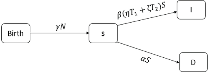
Representation of the susceptible couples.
Therefore, .
We show the treatment rate in the patient group with and the treatment rate of who were under medical treatment with . Therefore, the number of patients who used treatment is equal to . The number of people who left the clinic without any treatment is (Figure 2).
Figure 2.
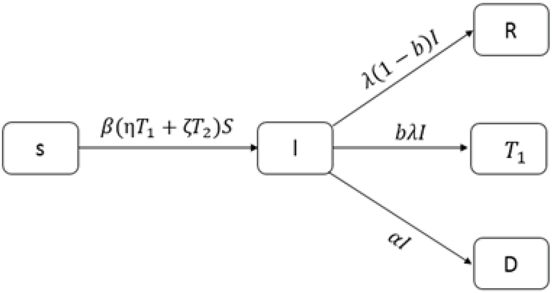
Patient couples are divided to three groups.
Hence .
We show the recovery rate in group with . We divide into two groups: the first group is the number of people who have recovered, and we show it with , in which is the recovery rate of at time . Therefore, of these people enters group. The number of people under medical treatment who left the clinic without any treatment is (Figure 3).
Figure 3.
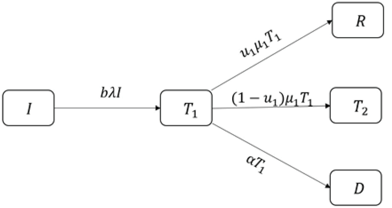
Infertile women under drug treatment.
Thus .
We show the recovery rate in group with . The recovery rate of at time is , therefore, the number of people treated with is equal to and the number of people under treatment entering group is equal to . The number of patients who left the clinic without any result is (Figure 4).
Figure 4.
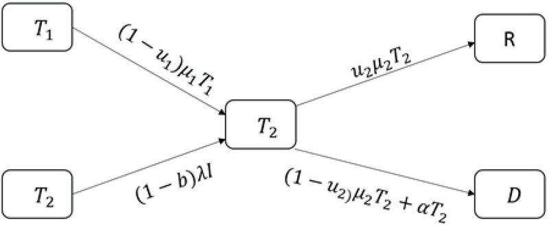
Infertile women under treatment.
According to Figure 4, we have: .
The number of susceptible people who left the group due to death is (Figure 5).
Figure 5.
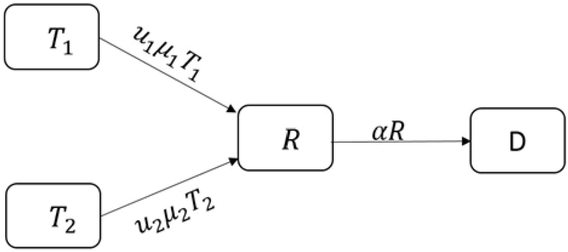
Cured infertile couples.
Hence
The number of infertile women who used cure methods is denoted by , and those entered susceptible at time by and denotes the number of infertile women who leave the population at time (Figure 6).
Figure 6.

All of the infertile couples.
According to the aforementioned cases, the dynamic model of infertile patients with can be modeled as follows:
We assume that the rate of return to the disease in each infertile women is the constant value of , and the number of secondary sufferers is equal to the number of infertile women who were treated, but returned to this disease afterward during the course of treatment. At first, we assume that the number of people in the population is equal to the number of people susceptible to the disease. To find , we replace , and with and deduce the following system.
This linear system is divided into two parts. The first matrix is shown by and is called returning matrix and the second matrix by , which is called affected matrix. Thus, if
then
Therefore,
where
and
is the trace of (5) Thus,
Analysis of women's infertility based on asymptotical stability
Based on the biological hypothesis, we can deduce model.
Prior to the disease, the free equilibrium point is , and we have the following result (6).
Theorem 2.1.1. If then:
a) If , then is the free equilibrium point which is locally stable but it is not asymptotically stable.
b) If , then the free equilibrium point is unstable.
c) If , then is locally asymptotically stable.
<statement> <title>Proof </title>
</statement>
(a) The linearized matrix of model at the point is
The characteristic equation of this matrix is:
The roots of this equation are:
Then, for other roots equation (3.3) using Routh Hurwitz methods (7). As all of the parameters are positive, . Moreover, .
We take
Additionally,
Since , then
Once again as , then
Hence,
Moreover, .
Since
Therefore,
By using (3.5) and (3.6), we obtain
Hence, by Hurwitz criterion, the real parts of the roots of (3.3) are all negative. If (3.2) is positive, then is not locally asymptotically stable.
(b) If (3.2) is zero, then is unstable.
(c) If , then the free equilibrium point is locally and asymptotically stable. (8, 9)
If , the number of patients who leave the clinic without result is less than the number of patients who enter the clinic. This demonstrates that considered treatment is useful. For a number of patients with Polycystic Ovary function, means local stability of free point; that is not asymptotically stable. If it shows the asymptotical stability of system, and it states that patients who come to the center have an acute infertility problem. If system is unstable, it means all the patients who come to the center leave there without any result. The evaulation of the treatment process depends on these three cases.
If
and
Where
Then, shows the other equilibrium point. Since the point is located in the interior of the positive space, we must have:
Sign stability of the dynamical model of women's infertility
When we model a biological phenomenon with differential equations, the values of the parameters used in them are error-prone. If we deal with a square matrix, then it is highly important to know how much the stability of this matrix depends on the elements of that matrix and how sensitive is it to the variations of the matrix elements. Therefore, in this section, using the following definitions and Theorems, we examine the sign stability of the system (1) at the equilibrium point of . To state the Theorem , we use some concepts of graph theory as follows.
Definition 2.2.1.(10): An square matrix A is said to be sign stable if every square matrix B of the same sign pattern (i.e., for all i; j = 1, 2,..., n) is a stable matrix.
For an square matrix A , we can obtain an undirected graph , whose vertex set is V = 1,2,..., n and edges are . Also, a directed graph DA can also attach to A with the same vertex set and edges . A k-cycle of is a set of distinct edges of of the form: : Let , which are the numbers for them the corresponding element in the main diagonal of the matrix is not zero. An -coloring of is a partition of its vertices into two sets, black and white (one of which may be empty). Such that each vertex in is black, no black vertex has precisely one white neighbor, and each white vertex has at least one white neighbor. A V complete matching is a set M of pairwise disjoint edges of such that the set of vertices of the edges in M contains every vertex in V . By applying this concepts, we are now able to state the following Theorem.
Theorem 2.2.2.(10): An real matrix A is sign stable if it satisfies the following conditions:
(i) for all i, j;
(ii) for all ;
(iii) The directed graph has no k-cycle for k ;
(iv) In every -coloring of the undirected graph all vertices are black; and
(v) The undirected graph admits a complete matching.
Theorem 2.2.3. If , then the matrix model at the equilibrium is not sign stable.
<statement> <title>Proof </title>
</statement>
The matrix of the linearize system model of at the equilibrium is given by
Where Theorem (2.2.2.) requires
Which is not sign stable. Since , then Theorem 2.2.2. implies that the matrix is not sign stable.
Theorem implies that in model at equilibrium point is not sign stable. This is a positive case from the perspective of the disease treatment, since the sign stability of model is equivalent to the return of disease, which has not been reversed for a long time; as a result, the problem of infertility and reproduction still remains for a high percentage of the population.
Reversibility of the infertility cycle with the PCOS factor in an model is not intermittent
The infertility treatment with initiates as a course of treatment with Clomiphene Citrate and Gonadotropin in some menstrual cycles, which, by the failure of medical treatment, changes the treatment with the therapy cycle. These patients will stay in that therapy course until they achieve the desirable result from it. From a medical point of view, this therapeutic cycle will not include the return to medical treatment during its treatment course. In this section, we prove that in system (1), the return of infertility is not circular in the cycle of the disease with the factor. In other words, the disease has no circulation.
First, we state the Stoke's Theorem.
Theorem 2.3.1. (Stoke's Theorem) (9): Suppose that is a bordered, oriented, compact, dimensional Manifold, and also suppose that is a smooth form on . In this case:
Where , as described earlier, is an oriented border.
Now, with the help of Stoke's Theorem, we state the Theorem on the closed circuits in this model.
Theorem 2.3.2. The model does not have a closed circuit.
<statement> <title>Proof </title>
</statement>
Assumption by contradiction: If there is a closed circuit like C with the rotation period of T, then we consider the Manifold M as a region in with the border C, and assume as a 5-form on M, which is defined as follows:
Therefore,
Hence, . However, it is concluded from Stoke's Theorem that and this is a contradiction. Therefore, the system (1) has no closed circuit; in other words, the reversibility of the therapeutic cycle of this disease is not intermittent.
Numerical solutions of the model
In this section, we solve model numerically via Rung-Kutta method (11). First, we define the following functions:
Hence,and are the initial conditions.
We take, where and for .
For we take
We put, and. So,
If and then we have the following graphs for the solutions.
Figures 7 and 8 are, respectively, considered for infertile women aged 20-25 and 25-30 with female factor and ovarian reserve of more than 3.5, based on the statistical data of Yazd Infertility Center. In Figure 8, is twice as in Figure 7; therefore, the number of the patients treated by in Figure 8 in its lowest amount (minimum) is half the number of patients treated by in Figure 7. The treatment duration of the patients in Figure 8 is approximately 1.5 times longer than that in patients in Figure 7. Moreover, and in Figure 7, and at the end of the cycle, have an incremental mode. The treatment speed of is more than that of , since the increase of age, the ovarian reserve decreases, and the medical treatment with clomiphene citrate and gonadotropin will no more be responsive. Therefore, the treatment with IVF is recommended to these patients. The evidences can exactly be observed in Figure 8. Similarly, the recovery speed of R in the Figure 7 reaches its minimum with no longer be responsive, to the extent that the minimum number of the improved patients in Figure 8 is approximately 0.25 of the number of the improved patients in Figure 7. In Figures 7 and 8, when R decreases, the number of patients increases.
Figure 9 has been reviewed for the patients with the ovarian reserve less than 3.5. In Figure 7, is twice more than the in Figure 9. Therefore, the number of the improved patients R in Figure 8 at its lowest value is almost twice as much as than the number of improved individuals in Figure 9. The length of treatment period in Figure 8 is approximately 1.5 times more than the length of treatment in Figure 9, since the speed of referral to the clinic, shown by, with respect to the ovarian reserve in Figure 8, is four times more than that in Figure 8.
Figure 7.
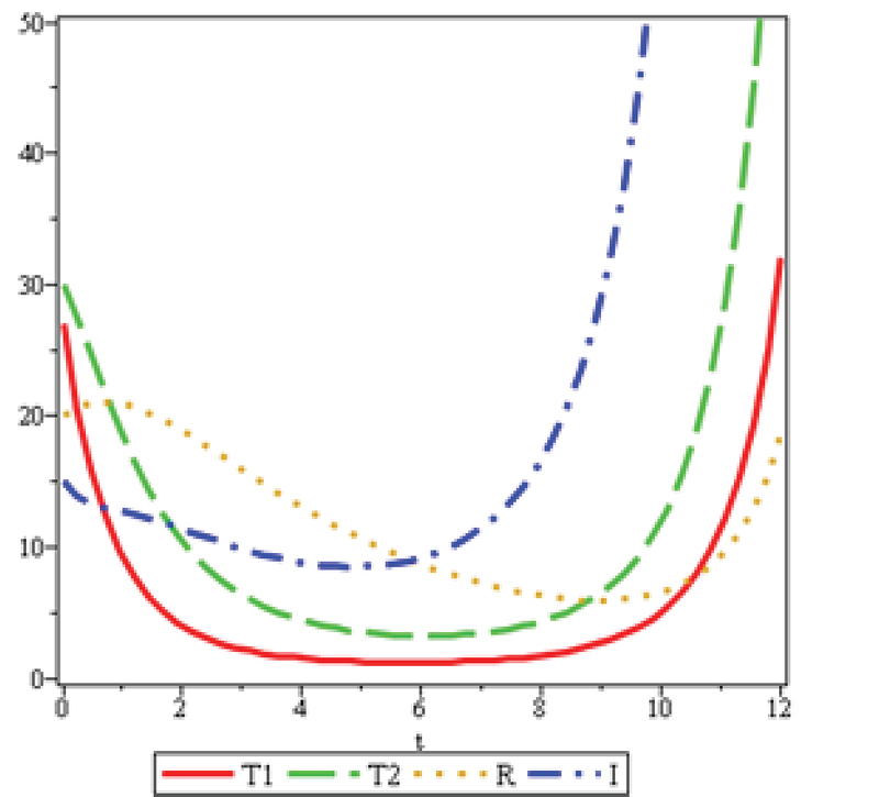
, and
Figure 8.
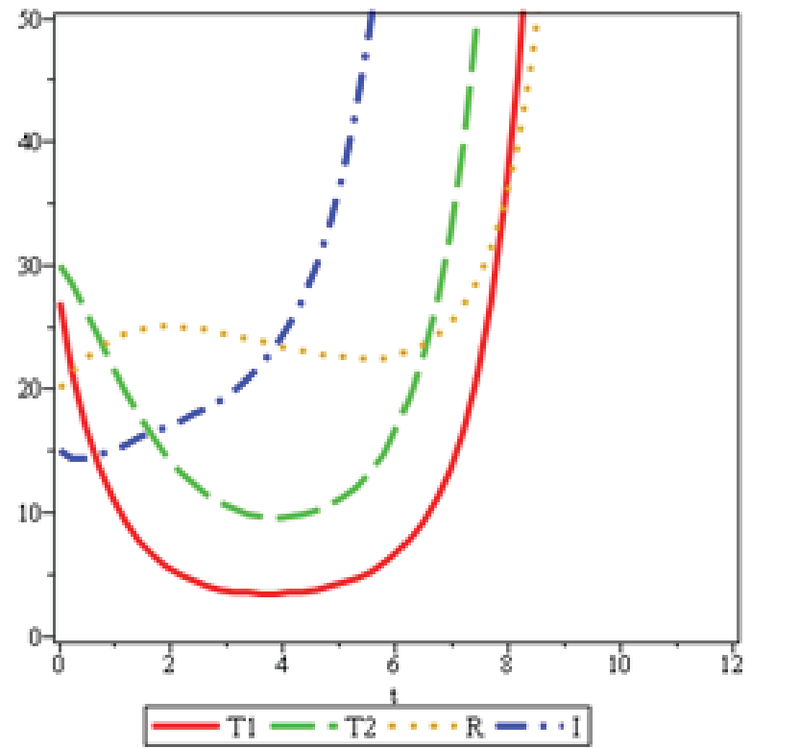
and .
Figure 9.
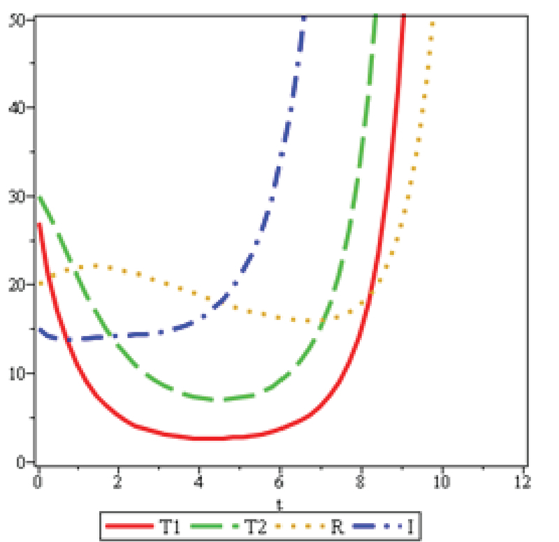
, and .
3. Discussion
The analysis of mathematical models depends on the sustainability of the disease in the community. In this model, the population volume is considered constant at a constant time and provides a good estimate for short periods with similar patients' conditions. Information obtained from the Yazd Infertility Center confirms that the ovarian reserve decreases as the age increases, thus, the number of patients attending IVF treatment increases, as seen clearly in Figures 7 and 8.
4. Conclusions
In this research, model is considered to cure infertility in couples. It is proved that the disease free equilibrium point for model is locally stable and it is not asymptotically stable, when. Here, is the number of patients who during treatment come across with the illness for the second time, and return to the clinic for secondary treatment. Furthermore, by using the Rung-Kutta method, we solved the model for achieving numerical solution. Considering the numerical results, the patients with ovariarn reserve less than 3.5 with two category of age range 20-25 and 25-30, it is shown that as age increases the ovarian reserve decreases, hence, Clomiphene Citrate and Gonadotropin treatments are not responsive. Obviously, IVF treatment is recommended in this group of patients. The main achievement of this study was that more ovarian reserve resulted in more cured infertile patients.
Conflict of Interest
The authors declare that they have no competing interests.
Acknowledgments
The authors would like to thank Professor Abbas Aflatoonian for his medical advice.
References
- 1.Vahidi Serajeldin, Ardalan Ali, Mohammad Kazem. Prevalence of Primary Infertility in the Islamic Republic of Iran in 2004-2005. Asia Pacific Journal of Public Health. 2009;21(3):287–293. doi: 10.1177/1010539509336009. [DOI] [PubMed] [Google Scholar]
- 2. Fritz MA, Speroff L. Clinical gynecologyic endocrinology and infertility. 8th Ed; Wolters Kluwer; Philadelphia: 2011.
- 3. Revised 2003 consensus on diagnostic criteria and long-term health risks related to polycystic ovary syndrome (PCOS) Human Reproduction. 2004;19(1):41–47. doi: 10.1093/humrep/deh098. [DOI] [PubMed] [Google Scholar]
- 4. Molaei MR, Waezizadeh T, Rezaeezadeh M. A mathematical model for HAV. U.P.B. Sci. Bull 2013; 75: 47-56.
- 5. Diekmann O, Hessterbeek JA, Matz JA. On the definition and the computation of the basic reoroduction ratio R0 in the models for infectious diseases in hetrrogeneous populations. J Math Biol 1990; 28: 356-382. [DOI] [PubMed]
- 6. Taherian M, Toomanian M, Molaei M. Two dynamical models for cholera, Theor Biol Forum 2016; 109: 131-148. . [DOI] [PubMed]
- 8.Li Xue-Zhi, Zhou Lin-Lin. Global stability of an SEIR epidemic model with vertical transmission and saturating contact rate. Chaos, Solitons & Fractals. 2009;40(2):874–884. doi: 10.1016/j.chaos.2007.08.035. [DOI] [Google Scholar]
- 9. Chern SS, Chen WH, Lam KS. Lectures on differential Geometry. World Scientific Publishing Co. Pte . Ltd 2000.
- 10. Farkas M. Dynamical models in biology, Academic Press; 2001.
- 11. Dahlquist G, Bjorck A, Anderson N. Numerical methods Prentice-Hall. Inc., Englewood Cliffs 1974.


