Rigid Motion Correction for Brain PET/MR Imaging using Optical Tracking

Abstract

A significant challenge during high-resolution PET brain imaging on PET/MR scanners is patient head motion. This challenge is particularly significant for clinical patient populations who struggle to remain motionless in the scanner for long periods of time. Head motion also affects the MR scan data. An optical motion tracking technique, which has already been demonstrated to perform MR motion correction during acquisition, is used with a list-mode PET reconstruction algorithm to correct the motion for each recorded event and produce a corrected reconstruction. The technique is demonstrated on real Alzheimer’s disease patient data for the GE SIGNA PET/MR scanner.

I. Introduction

A typical PET/MR brain scan lasts between 10–60 minutes, with the PET acquisition generally spanning the entire scan time. Any head motion with a magnitude of a similar order to the PET spatial resolution (i.e. millimetres) will result in a blurring of the final reconstructed image. While the subject’s head is usually restrained in the head coil to mitigate motion, most subjects nonetheless exhibit some motion, particularly in the axial direction. It is common to perform a retrospective, frame-by-frame motion correction technique. This works well when there is sporadic motion (for example, after the patient coughs, the position of the head may change). If patient motion is erratic (for example, for a patient with a motion disorder), a frame-by-frame motion correction scheme may not work adequately. This problem is exacerbated on a PET/MR system, where, given the duration of the PET scan during a PET/MR study, the tracer dose is generally minimised to reduce the patient radiation exposure. Therefore there are usually insufficient event statistics to reliably perform a frame-by-frame motion correction scheme using an adequately high frame-rate.

Although motion correction (MC) for brain imaging has been present in the literature since the early 1990’s, it has still not found its way into standard clinical routine. The theory of how to perform a reconstruction with MC has largely been reported [1], [2], and therefore most current reports on MC focus on various implementations of the technique. Abdominal motion is a more complicated problem, and both the methods for motion estimation and image reconstruction are still being developed in the literature. A recent review of the latest developments for both head and abdominal motion correction can be found in [3] and [4], together with another important earlier review in [5].

The absence of MC from standard clinical routine of brain studies can be attributed to two major factors:

• Poor PET image resolution: Until recently, the spatial resolution of reconstructed PET images was such that small motions of the head would not add significant blurring to the image; therefore, motion correction was seen as an unnecessary complication.

• Inadequate motion tracking technology: The motion trackers used to date have either imposed a significant additional burden on the procedure for the scan setup for either the technologists or the patient, or the robustness and reliability of the trackers have been lacking.

With modern PET scanners, however, a spatial resolution of 4 mm is becoming common, such that even small motions with a magnitude of only ~2 mm can cause noticeable image degradation, and modern motion trackers have reached the point where the additional burden of the clinical routine is negligible or absent, while becoming much more robust.

Huang et al. presented a head motion tracker for a PET/MR system which used microcoils attached to a phantom which can be tracked by the MR system [6]. MR navigators (fast, 1 or 2 dimensional acquisitions) have also been used to track head motion, for example in [7]; these usually require fairly complicated MR sequences in order to allow the MR to still be clinically available for uses other than just motion tracking, and no motion information is available at times when the MR is not active. Modern, external optical tracking devices currently offer very robust and accurate motion estimates while imposing a minimal intrusion into the clinical routine or MR sequences. Several trackers which avoid the use of markers on the patient have been presented (e.g. [8], [9], but this is difficult to achieve robustly within the small confines of a head coil.

Recently, an optical motion tracking system was developed for the GE SIGNA PET/MR (GE Healthcare, Waukesha, WI, USA) to perform real time motion correction for the MR data [10], [11]. The recorded motion data are used to reorientate the MR gradients in real time to correct for the measured motion. The tracker has been developed to have a minimal effect on the standard clinical procedure. The scheme was then extended to use the same recorded motion data to correct each measured PET event for motion before performing a list-mode PET reconstruction [12]. To the best of our knowledge this is the first time that a motion correction scheme is implemented which corrects both the PET and MR during a simultaneous scan, using the same motion data. Our aim in this work was to demonstrate the application of this scheme in the clinical setting with Alzheimer’s disease patients.

In addition we show results from an investigation into the effect of the subset size on a list-mode PET reconstruction.

II. Method

A. Optical Tracker

An MR-safe, external tracker, developed by HobbitView Inc. in collaboration with GE Healthcare, was used to record the motion data [10], [11]. This device consists of a single optical camera attached directly to the head coil of the PET/MR scanner. It tracks a large, curved marker temporarily attached to the patient’s forehead. The attachment of the marker is a very simple task and does not cause any discomfort to the patient. The marker is covered in a checkerboard-like pattern with half the squares containing a unique coded symbol which allows the tracking software to identify the square’s location on the marker. The tracker only needs to see some of these squares to generate a position estimate. This permits a large range of motion, particularly for lateral rotations. The tracker reports the 6 degrees-of-freedom (3 translations and 3 rotations) of the marker for each motion data point. The motion of the marker is assumed to correspond to the motion of the brain. While it is possible for the marker to move with the skin and thus relative to the brain, as is discussed in [11] this is mitigated by the size of the marker and the large area of attachment on the forehead; over many studies involving many patients this has not been observed to be a noticeable problem.

The tracker operates at a frequency of 40 — 100 Hz. A spatial calibration between the tracker and the scanner is performed once, and the tracker is rigidly and reliably reattached in the same position on the head coil for each scan [13]. Temporal synchronisation is achieved by the fact that both the scanner and the tracker use the same timing system for their start times, and is accurate to within 1 ms.

B. List-mode Algorithm

The motion data is used to transform the endpoints of each list-mode event at the corresponding times, thereby correcting for the head motion. A list-mode reconstruction algorithm [14], [15] is then performed using the following formulation:

$${\lambda }_j^{n+1}=\frac{{\lambda }_j^n}{{\tilde{s}}_j}\sum _m{c}_{i_m^{\prime }j}\frac{1/I_{i_m^{\prime }}}{\sum _k{c}_{i_m^{\prime }k}{\lambda }_k^n+\frac{S_{i_m}+R_{i_m}}{a_{i_m}{s}_{i_m}}},$$ (1)

where ${\lambda }_j^n$ is the image value at pixel j and iteration n, C_ij is the system matrix, i_m is the line-of-response (LOR) i associated with list-mode event m (note that we use LOR to refer to a line defined by any two points), with $i_m^{\text{'}}$ being that LOR after motion correction, I_i is the in vivo attenuation correction factor for LOR i, a_i is the combined in vivo and hardware attenuation correction factor, S_t and R_i are the scatter and randoms contributions, respectively, and ${\tilde{s}}_j$ is the time-averaged sensitivity image, given by (as proposed in [1]):

$${\tilde{s}}_{j^{\prime }}=\sum _p\frac{1}{w_p}\sum _j{T}_{p,j^{\prime }j}\sum _i{c}_{ij}{H}_i{\sigma }_i,$$ (2)

where w_p is the weighting (i.e. fractional duration) of motion data point p, T_{ρ, j’j} is the transformation matrix for motion data point p from pixel j to j’, H_i is the hardware attenuation correction factors for LOR i, and σ_i is the scanner sensitivity factors for LOR i. Note that the in vivo and hardware attenuating materials are treated separately since the former exhibits motion while the latter do not.

Both the MR and PET data are corrected to the same reference frame. They are therefore automatically aligned to each other which avoids any mismatch between the PET image and the attenuation map.

C. Point Spread Function Modelling

The implemented projectors project a tube-of-response (TOR) along the LOR defined by an event’s endpoints. The cross-section of the TOR varies in both directions orthogonal to the LOR. In the transaxial plane the TOR accounts for the crystal size and depth-of-interaction effect, which varies with radial position in the scanner. In the axial plane a static and symmetrical kernel is used. The spatially variant point spread function (PSF) model persists correctly with motion correction.

D. Subset Selection

Subsets are used to accelerate the reconstruction algorithm [16]. For list-mode reconstruction, one can choose the subsets as a fraction of the total number of measured events, with all subsets being mutually exclusive and exhaustive. It is assumed that the number of events in each subset is large enough such that each subset is statistically representative of the entire set. Therefore the sensitivity image is calculated using all possible LORs in the scanner, and then scaled by the number of subsets. We identified two important aspects of using subsets, in a list-mode reconstruction in particular, that require careful consideration, namely: the scheme used to select the subsets, and the effect of the size of the subset on the reconstruction.

a). Subset Selection Scheme:

There are two obvious schemes for selecting the subsets: selecting temporally contiguous subsets of events, or distributing the events evenly in time among the subsets by placing each subsequent event in each subsequent subset and looping through the subsets to the end of the data set. The distributed scheme has a number of advantages over the contiguous scheme:

• the noise statistics of each subset are approximately the same;

• the correction factors are identical for each subset (scatter, randoms, decay, duration, etc.);

• if there is motion, the motion present in each subset is almost exactly the same.

Therefore the distributed subset selection scheme is used in this work.

b). Subset Size:

For a list-mode reconstruction, a subset must be thought of slightly differently to a sinogram reconstruction. If we consider a particular scan type (e.g. neu-roimaging with FDG), and if we allow for a certain amount of noise in each subset, then we could (in theory) decide that E list-mode events are statistically representative of the whole data set. That number, E, depends on aspects such as the activity distribution, and is independent of the total number of measured events in the data set. (Note that randoms complicate this assumption since they have a different relationship to the count rate than the true coincidences do, but this is beyond the scope of the current work and will be investigated in the future.) Therefore we could keep E constant across data sets of similar scan types, and for large data sets we would have many subsets, and for small data sets would have few subsets. The noise level in all subsets though, across the data sets, would be similar, leading to similar convergence properties. This is somewhat different to a sinogram reconstruction where subsets of the same size across different data sets might have different noise properties. In this investigation we try to determine a lower bound for this E for a particular test case of the NEMA image quality phantom.

We will use the term “image update” to refer to the processing of one subset during the reconstruction, with the total number of image updates therefore being the product of the number of iterations and subsets. This total number of updates gives a rough indication of the convergence level reached. The number of list-mode events used per update, E, can be any factor of the total number of events, N. By decreasing E more image updates are performed per iteration. Therefore, for a given number of updates, with a lower E fewer iterations are required, which implies a faster reconstruction (with respect to time) since each iteration is one full pass through the data set. If E is too small, however, the subsets may be significantly different from each other, which may negatively impact the reconstruction.

III. Experiments & Studies

A NEMA image quality phantom was scanned in a GE SIGNA PET/MR scanner (GE Healthcare, Waukesha, WI, USA) with an injected activity of 71 MBq of ¹⁸F-FDG (contrast of 4:1) for 10 minutes in order to test the effect of the number of events per update on the reconstruction.

Three point sources were rigidly attached to each other and moved in the scanner to test the efficacy of the motion correction scheme.

A patient with Alzheimer’s disease underwent a brain scan for 75 minutes after being injected with 341 MBq of ¹⁸F-florbetaben¹, while their head motion was being tracked. The following MR sequences with motion correction capability were acquired: GRE, IR-SPGR and resting state fMRI. Both the PET and MR acquisitions were corrected for motion to demonstrate the feasibility of the scheme within the clinical setting.

The attenuation map for the PET reconstruction was generated using an atlas which is adjusted according to MR data acquired during a sequence specifically for this purpose. This was the standard protocol for this scanner at the time this data was acquired.

The tracker itself is currently not incorporated into the attenuation map since it is constructed using very lightly attenuating materials, with the mass of the entire prototype assembly just over 160 g. However, in the future the camera system will be embedded in the head coil and will then automatically be included in the attenuation map for the coil.

IV. Results

A. Subset Size Investigation

The NEMA phantom data set contained 650 million listmode events. The data was reconstructed using 9 different number of events of per update (E) ranging between approximately 1 and 108 million events (corresponding to 650 and 6 subsets per iteration, respectively). While this may seem like a large number of subsets, recall that for list-mode reconstruction the important parameter is E, regardless of the size of the data set, and by extension therefore the number of subsets. We wanted to investigate a wide range of values for E, and for this particular data set that implied a large number of subsets for a small E.

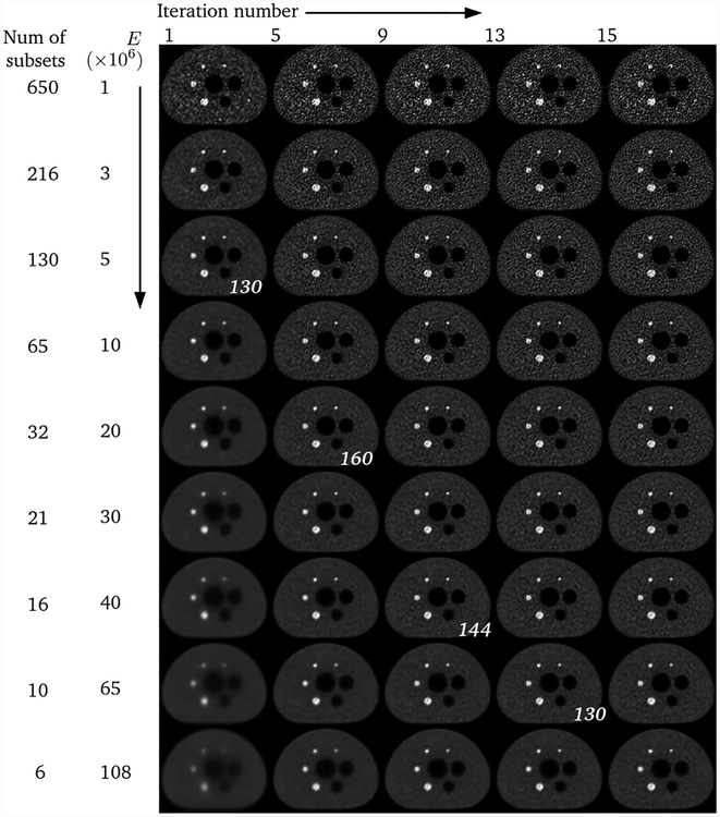
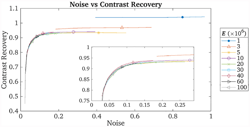
Figure 1 shows the results of these reconstructions. In the first row, convergence seems to have been reached within the first few iterations (since there were 650 updates per iteration) but the noise level is high. In the last row, on the other hand, convergence has been slow (since there are only 6 updates per iteration). Figure 2 shows the noise versus contrast recovery metrics for these reconstructions. The background region-of-interest (ROI) was comprised of 3 cylindrical regions in the warm section of the phantom, and the contrast recovery was calculated using the 22 mm hot sphere. The convergence paths for reconstructions with E ≥ 5 ×10⁶ events all lie approximately on top of each other, implying that these reconstructions all reach a similar result but with differing convergence rates with regards to the iteration number. The reconstructions with E ≤ 3 × 10⁶ events seem to exhibit a positive bias. A likely explanation is that, when E is very low, the assumption that each subset is statistically representative of the whole data set is no longer true, and noise is introduced into the reconstruction by each subset differing significantly from the others. Such noise could cause noise-induced bias, which is a known characteristic of OSEM. Therefore we can conclude that the reconstruction after a given number of updates is independent of E for E ≥ 5 × 10⁶ events.

Fig. 1.

Each row shows a different reconstruction of the NEMA phantom data using increasing E (and therefore decreasing number of subsets), with increasing number of iterations for each reconstruction from left to right. The italicised numbers indicate reconstructions with similar number of updates, which should therefore be comparable in image quality.

Fig. 2.

Plot of image noise versus contrast recovery for the 22 mm hot sphere for reconstructions with varying E. The symbols indicate the values at iteration 8. The inset shows that the plots for E ≥ 5 × 10⁶ all lie approximately on top of each other.

B. Moving Point Sources

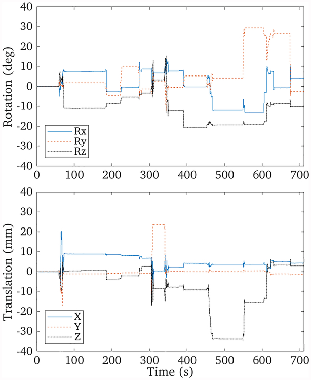
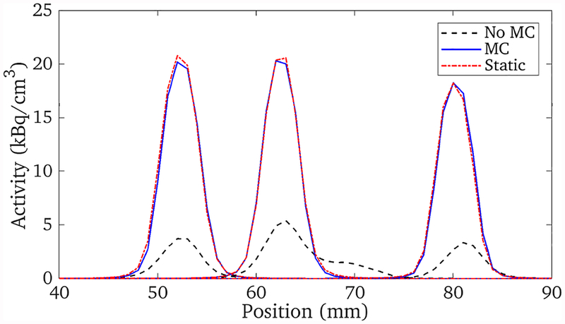
The three point sources were moved with a range of approximately ±30° and ±30 mm, with motion along all 6 DOFs, as shown in figure 3. The data set consisted of 10 million events spanning 700 seconds. Figure 4 shows the results of the list-mode reconstructions of the data with and without motion correction, as well as a reconstruction of a stationary data set acquired just prior to that with motion. The profiles through these reconstructions are shown in figure 5. The full-width at half maximum of the stationary and motion corrected reconstructions for the three point sources agreed with each other to within 1%.

Fig. 3.

Tracked motion data of the three point sources over the 700 second scan. A large range of motion was exhibited

Fig. 4.

Maximum intensity projections of the reconstructions of the point source data. The left and middle reconstructions are of the same data set but without and with motion correction, respectively. The right reconstruction is of the stationary data set, whose position and orientation were used as a reference frame for the motion corrected reconstruction in the middle. The white lines indicate the locations of the profiles shown in figure 5.

Fig. 5.

The profiles through the reconstructions shown in figure 4. The motion corrected and stationary data reconstructions agree with each other very closely.

The reference frame for the motion corrected reconstruction was that of the stationary data. Therefore the final reconstruction is well aligned with the stationary reconstruction without any need for further image registration. This demonstrates that, for clinical studies, the PET data can be corrected to the reference frame of the attenuation map to ensure that these are well aligned.

C. Patient Studies

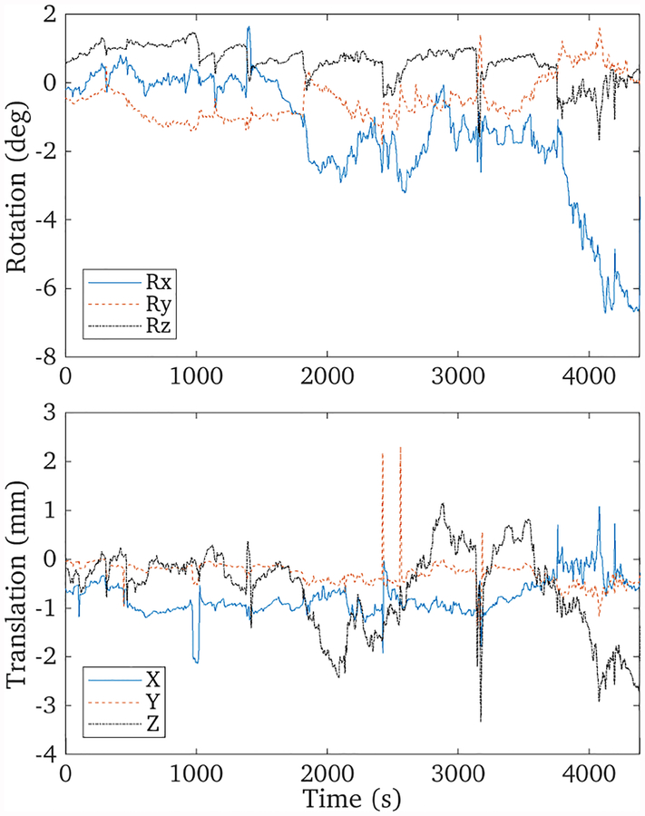
The recorded motion of the patient’s head is shown in figure 6. The motion ranges between [—8, 2]° and [—3, 2] mm, and substantial motion was observed in the final 10 minutes of the scan. The extent of this patient’s motion was, however, considerably less than is often observed with Alzheimer’s disease patients.

Fig. 6.

Tracked motion data of the patient brain scan over the 70 minute scan. Substantial motion can be observed in the last 10 minutes of the scan, corresponding to a nodding motion of the head.

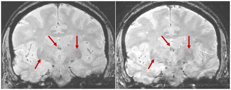
Figure 7 shows the results of applying motion correction during the MR acquisition using the GRE sequence. The two data sets shown were acquired sequentially, with and without motion correction. A motion artefact is not present in the corrected reconstruction, and the spatial resolution of the image has improved with motion correction. These data were acquired simultaneously with the PET data.

Fig. 7.

Comparing GRE images with (left, TR = 2500 ms) and without (right, TR = 2700 ms) motion correction (both: TE = 20 ms, FOV = 24 × 18 cm, slice thickness = 2 mm, inter-slice spacing = 0 mm, matrix = 384 × 256). The arrows indicate motion artefacts which are absent with motion correction.

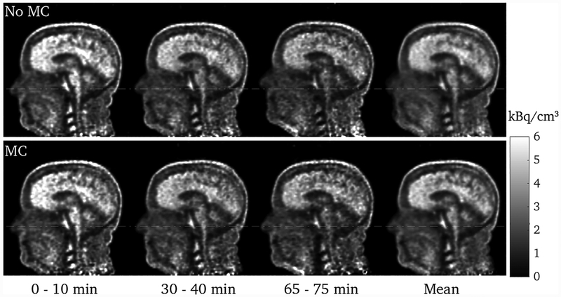
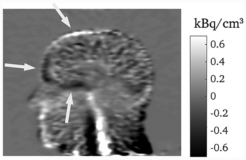
The full PET list-mode data set consisted of 1.2 × 10⁹ events. Reconstructions of 10 minute frames from the beginning, middle, and end of the scan are shown in figure 8, each containing 210, 150, and 110 million events, respectively. The upward nodding motion of the head can be observed in the last 10 minute frame, and this has been corrected for with motion correction. Since the attenuation map corresponds to the head in the position at the beginning of the scan, the motion in the last 10 minutes causes a mismatch between the data and the attenuation map in the uncorrected reconstruction. The effect of this is demonstrated in figure 9: the non-MC reconstruction has been registered to the MC reconstruction, and the difference image taken; this difference image shows the quantitative differences due to the attenuation mismatch in the non-MC reconstruction.

Fig. 8.

Sagittal slices through the head for frames at the beginning, middle, and end of the scan, and the mean of these three, without (top) and with (bottom) motion correction. The white dashed line is a visual guide. The motion is most evident by the lifting of the nose. The effect of the head motion has clearly been much reduced with motion correction.

Fig. 9.

Difference image for the last 10 minute frame between the MC reconstruction and the non-MC reconstruction after it has been registered to the MC reconstruction. The differences in quantification indicated by the arrows are due to the mismatch between the emission data and the attenuation map in the non-MC reconstruction.

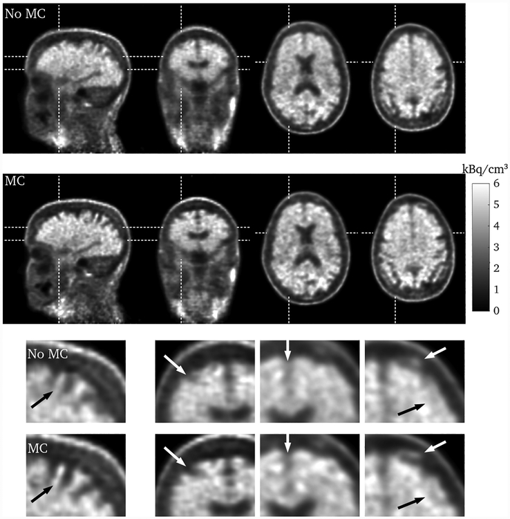
Figure 10 shows sagittal, coronal, and transverse slices through the brain for the entire scan duration. Certain regions of the brain can be better resolved after motion correction, in particular the definition of the gyri. In this case the motion of the patient’s head was not as extensive as is often observed, but the motion correction nevertheless has had a substantial effect.

Fig. 10.

Sagittal, coronal, and two transverse slices through the brain for the entire scan duration, without (first row) and with (second row) motion correction. The bottom two rows show zoomed in sections of the images. The dashed lines indicate from where the slices are taken, and the red arrows highlight regions where the effect of the motion correction can be seen.

V. Conclusion

We have presented a rigid motion correction scheme which uses an external, marker-based, optical camera to track the motion of the patient’s head and then perform motion correction on both the MR (prospectively, in real-time) and on the PET data (during reconstruction). The motion correction of the PET data is performed on an event-by-event basis and a list-mode reconstruction is conducted.

The choice of the number of events to use per update (E) for the list-mode reconstruction was investigated. It was found that for E ≥ 5 ×10⁶ the resulting reconstructions were independent of E at a given number of updates. Using a low E is desirable since it implies that, to perform a certain number of updates, fewer iterations are required. Our investigation therefore puts a lower bound on E.

The efficacy of the motion correction scheme was demonstrated with moving point source data. It was further demonstrated that the scheme works well within a clinical setting by implementing it during the scan of a patient with Alzheimer’s disease. Motion artefacts were removed and the spatial resolution enhanced for both the MR and PET data.

With some further refining and dissemination to other research sites for testing, it is our hope that head motion correction will soon become more commonly used in standard clinical practice.

References

- [1].Rahmim A, Bloomfield P, Houle S, Lenox M, Michel C, Buckley KR, Ruth TJ, and Sossi V, “Motion compensation in histogram-mode and list-mode EM reconstructions: beyond the event-driven approach,” IEEE Transactions on Nuclear Science, vol. 51, no. 5, pp. 2588–2596, 2004. [Google Scholar]
- [2].Carson RE, Barker WC, Liow J-S, and Johnson CA, “Design of a motion-compensation OSEM list-mode algorithm for resolution-recovery reconstruction for the HRRT,” in IEEE Medical Imaging Conference Proceeding, vol. 5, 2003, pp. 3281–3285. [Google Scholar]
- [3].Gillman A, Smith J, Thomas P, Rose S, and Dowson N, “PET motion correction in context of integrated PET/MR: Current techniques, limitations, and future projections,” Medical Physics, vol. 44, no. 12, pp. e430–e445, 2017. [DOI] [PubMed] [Google Scholar]
- [4].Catana C, “Motion correction options in PET/MRI,” in Seminars in Nuclear Medicine, vol. 45, no. 3 Elsevier, 2015, pp. 212–223. [DOI] [PMC free article] [PubMed] [Google Scholar]
- [5].Rahmim A, Rousset O, and Zaidi H, “Strategies for motion tracking and correction in PET,” PET clinics, vol. 2, no. 2, pp. 251–266, 2007. [DOI] [PubMed] [Google Scholar]
- [6].Huang C, Ackerman JL, Petibon Y, Brady TJ, El Fakhri G, and Ouyang J, “MR-based motion correction for PET imaging using wired active MR microcoils in simultaneous PET-MR: Phantom study,” Medical Physics, vol. 41, no. 4, 2014. [DOI] [PMC free article] [PubMed] [Google Scholar]
- [7].Keller SH, Hansen C, Hansen C, Andersen FL, Ladefoged C, Svarer C, Kjær A, Højgaard L, Law I, Henriksen OM et al. , “Motion correction in simultaneous PET/MR brain imaging using sparsely sampled MR navigators: a clinically feasible tool,” European Journal of Nuclear Medicine and Molecular Imaging: Physics, vol. 2, no. 1, p. 14, 2015.26501815 [Google Scholar]
- [8].Olesen OV, Sullivan JM, Mulnix T, Paulsen RR, Hojgaard L, Roed B, Carson RE, Morris ED, and Larsen R, “List-mode PET motion correction using markerless head tracking: Proof-of-concept with scans of human subject,” IEEE Transactions on Medical Imaging, vol. 32, no. 2, pp. 200–209, 2013. [DOI] [PubMed] [Google Scholar]
- [9].Kyme AZ, Maclaren J, Aksoy M, and Bammer R, “Feasibility of marker-free motion tracking for motion-corrected MRI and PET-MRI,” in IEEE Medical Imaging Conference Proceeding, 2016, pp. 1–3. [Google Scholar]
- [10].Aksoy M, Forman C, Straka M, Skare S, Holdsworth S, Hornegger J, and Bammer R, “Real-time optical motion correction for diffusion tensor imaging,” Magnetic Resonance in Medicine, vol. 66, no. 2, pp. 366–378, 2011. [DOI] [PMC free article] [PubMed] [Google Scholar]
- [11].Aksoy M, Maclaren J, and Bammer R, “Prospective motion correction for 3D pseudo-continuous arterial spin labeling using an external optical tracking system,” Magnetic Resonance Imaging, vol. 39, pp. 44–52, 2017. [DOI] [PMC free article] [PubMed] [Google Scholar]
- [12].Spangler-Bickell M, Maclaren J, Aksoy M, Khalighi M, Bammer R, Rettmann D, Tohme M, Jansen F, and Nuyts J, “Rigid motion correction for PET brain imaging during simultaneous PET/MR,” ISMRMworkshop on Motion Correction in MRI and MRS, Cape Town, South Africa, September 2017. [Google Scholar]
- [13].Maclaren J, Aksoy M, Ooi MB, Zahneisen B, and Bammer R, “Prospective motion correction using coil-mounted cameras: Crosscalibration considerations,” Magnetic Resonance in Medicine, vol. 79, no. 4, pp. 1911–1921, 2018. [DOI] [PMC free article] [PubMed] [Google Scholar]
- [14].Reader AJ, Erlandsson K, Flower MA, and Ott RJ, “Fast accurate iterative reconstruction for low-statistics positron volume imaging,” Physics in Medicine & Biology, vol. 43, no. 4, p. 835, 1998. [DOI] [PubMed] [Google Scholar]
- [15].Parra L and Barrett HH, “List-mode likelihood: EM algorithm and image quality estimation demonstrated on 2-D PET,” IEEE Transactions on Medical Imaging, vol. 17, no. 2, pp. 228–235, 1998. [DOI] [PMC free article] [PubMed] [Google Scholar]
- [16].Hudson HM and Larkin RS, “Accelerated image reconstruction using ordered subsets of projection data,” IEEE Transactions on Medical Imaging, vol. 13, no. 4, pp. 601–609, 1994. [DOI] [PubMed] [Google Scholar]