A framework for uncertainty and risk analysis in Total Maximum Daily Load applications

Abstract

In the United States, the computation of Total Maximum Daily Loads (TMDL) must include a Margin of Safety (MOS) to account for different sources of uncertainty. In practice however, TMDL studies rarely include an explicit uncertainty analysis and the estimation of the MOS is often subjective and even arbitrary. Such approaches are difficult to replicate and preclude the comparison of results between studies. To overcome these limitations, a Bayesian framework to compute TMDLs and MOSs including an explicit evaluation of uncertainty and risk is proposed in this investigation. The proposed framework uses the concept of Predictive Uncertainty to calculate a TMDL from an equation of allowable risk of non-compliance of a target water quality standard. The framework is illustrated in a synthetic example and in a real TMDL study for nutrients in Sawgrass Lake, Florida.

1. Introduction

Section 303(d) of the U.S. Clean Water Act identifies a Total Maximum Daily Load (TMDL) as the maximum pollutant load that a water body can assimilate without violating a specific water quality standard. A TMDL is computed as the sum of the allowable loads from point and non-point sources ($\sum WLA$ and $\sum LA$, respectively) plus a margin of safety (MOS) as follows (U.S. Environmental Protection Agency, 1999; Shirmohammadi et al., 2006):

$$TMDL=\sum WLA+\sum LA+MOS$$ (1)

The MOS is a fraction of the TMDL which fundamentally accounts for the uncertainty in the modeling and calculation of the assimilative capacity of the water body. The main sources of this uncertainty are model structure uncertainty, input data uncertainty and model parameter uncertainty. The model structure uncertainty results from errors in model formulation and numerical solution of the equations describing a particular physical, biological or chemical process. Input data uncertainty results from errors in field and laboratory measurements used to force and calibrate the models. Finally, parameter uncertainty results from the use of inaccurate model parameter values. Given these multiple sources of uncertainty, the MOS represents a critical component of the TMDL. However, objective and standardized approaches for the computation of the MOS are limited.

Traditionally, the MOS has been either implicitly incorporated in a TMDL by using conservative assumptions for the estimation of the assimilative capacity of the water body or explicitly incorporated in the TMDL as an independent load allocation as in Eq. (1) (U.S. Environmental Protection Agency, 1991). The lack of an objective approach for the computation of the MOS has resulted, however, in a wide range of subjective and often arbitrary criteria for its computation which in most cases cannot be replicated nor used for comparative analyses between TMDL studies. In addition, the use of subjective approaches generally result in unclear relationships between the TMDL and the MOS and more importantly between the MOS and the water quality standards. The limitations of using subjective approaches for the computation of the MOS have been documented by several researchers including Dilks and Freedman (2004) in a review of 172 TMDLs performed in eight states, Langseth and Brown (2010) in a review of 50 TMDLs from New England, and Crumpacker and Butkus (2009) in a review of 23 TMDLs from the states of Washington, Oregon, and California. Langseth and Brown (2010) point out that none of the TMDLs reviewed in their study explicitly consider the risk of violating the water quality standards as the basis to define the MOS.

To overcome the limitations of the subjective approaches the National Research Council recommends the use of objective uncertainty analyses as the basis for the MOS and TMDL calculation (NRC, 2001). This recommendation is also supported by several researchers and practitioners who also advocate the use of uncertainty analysis as a more transparent, reproducible and robust strategy to define the MOS and TMDL (Ames and Lall, 2008; Dilks and Freedman, 2004; Langseth and Brown, 2010; Liang et al., 2016; Reckhow, 2003; Shirmohammadi et al., 2006). Dilks and Freedman (2004) argued that an objective uncertainty-based-method to compute the MOS and TMDL should have four important attributes. First, the method should explicitly account for the impacts of uncertainty on the estimation of the MOS and TMDL. Second, the method should be reproducible. Third, the method should explicitly define the degree of protection expected from the TMDL as the probability that the water quality standard will be satisfied once the TMDL is implemented. And fourth, the method should identify data limitations and also implementation problems that could result from TMDLs computed under limited data availability or with the use of poor quality datasets. This latter aspect, however, is more related with policy making and requires stakeholder involvement during the definition of the TMDLs.

To incorporate explicit uncertainty analyses in the TMDL process, research has been conducted to compute the MOS and TMDL based on methods such as First Order Variance Analysis (Park and Roesner, 2012; Zhang and Yu, 2004), Point Estimation Methods (Franceschini and Tsai, 2008), Bayesian Networks (Alameddine et al., 2011; Ames and Lall, 2008; Patil and Deng, 2011) and Risk Assessments (Borsuk et al., 2002; Gronewold and Borsuk, 2009; Hantush and Chaudhary, 2014; Langseth and Brown, 2010). Methods based on risk assessments and Bayesian inference have been subject of increasing attention during the last decade because they can be used to explicitly calculate the probability of non-compliance or failure of the TMDL due to multiple sources of uncertainty. Borsuk et al. (2002) presented a probabilistic and Bayesian approach to calculate the risk of non compliance and MOS of TMDLs assuming the errors between the model predictions and observations are independent, normally distributed and unbiased. More recently Ames and Lall (2008) developed a Bayesian network to obtain uncertainty and risk estimates for TMDLs; Gronewold and Borsuk (2009) developed a software tool to estimate the probability of compliance of TMDLs from deterministic model results; and Langseth and Brown (2010) developed a strategy to compute the MOS using risk based concepts traditionally used in engineering design, although their strategy does not include an explicit method for the propagation of uncertainty to model predictions. Hantush and Chaudhary (2014) extended the method proposed by Borsuk et al. (2002) for more general cases where the errors between the model predictions and the observations are correlated and biased and also computed the MOS from an equation of risk of non-compliance.

Risk-based approaches apply the concept of performance failure to compute a TMDL. In engineering, a system experiences a performance failure when it is unable to perform as expected (Singh et al., 2007). In the TMDL context, the probability of failure of the TMDL after implementation is known as the risk of non-compliance. This probability can be computed using a mathematical model, if the target concentration (c*) and also the allowed frequency of non-compliance (β) of a water quality standard are defined. Traditionally, the computation of a TMDL under a risk-based framework must satisfy:

$$P\left(Y>c^{*}|\mathbf{\text{θ}},\mathbf{X}\right)\le \beta$$ (2)

where $P\left(Y>c^{*}|\mathbf{\text{θ}},\mathbf{X}\right)$ is the probability that a simulated water quality variable Y will exceed c* given a vector of model parameters θ, and a matrix of input data X such as flows and contaminant loads from point and non-point sources (e.g. Borsuk et al., 2002; Hantush and Chaudhary, 2014). Risk based approaches based on Eq. (2) have, however, an important limitation. Eq. (2) assumes that the left side of the equation which represents the probability that the model predictions of a variable of interest (Y) will exceed the target concentration c*, is equal to the probability that the actual concentrations (Z) will exceed the target concentration c*, or $P\left(Z>c^{*}\right)$, which is the probability of interest for management purposes. The above is an inaccurate assumption because the model exceedance probability $P\left(Y>c^{*}|\mathbf{\text{θ}},\mathbf{X}\right)$ and the actual exceedance probability $P\left(Z>c^{*}\right)$ can only be equal if the model is a perfect representation of the real world and is able to reproduce observed concentrations with a 100% accuracy i.e. an ideal case. In reality $P\left(Y>c^{*}|\mathbf{\text{θ}},\mathbf{X}\right)<>P\left(Z>c^{*}\right)$ and thus, a reformulation of Eq. (2) is necessary to have an accurate assessment of the risk of failure of the TMDL i.e. $P\left(Z>c^{*}\right)$ and also a more accurate basis for the MOS computation.

This investigation has three main objectives. The first objective is to reformulate Eq. (2) to obtain a more accurate assessment of the probability that the real world observations will exceed the target concentration $P\left(Z>c^{*}\right)$, i.e. the TMDL risk of failure. The second objective is to present a Bayesian strategy to solve the resulting equation for $P\left(Z>c^{*}\right)$; and the final objective is to propose a strategy to compute the MOS and TMDL that satisfy an allowable risk of non-compliance (β).

The proposed approach to calculate $P\left(Z>c^{*}\right)$ incorporates a Bayesian parameter inference strategy to explicitly account for the impacts of model and parametric uncertainty. The Bayesian parameter inference is based on the likelihood function recently proposed by Hantush and Chaudhary (2014) which is relatively general for most practical cases. The method is demonstrated in a theoretical biochemical oxygen demand TMDL using the estuarine Streeter-Phelps model, and in a real application of the Water Quality Analysis Simulation Program (WASP) (Ambrose et al., 1993) to determine a nutrient TMDL in Sawgrass Lake, Florida, USA. The paper is organized as follows. Section 2 formulates the Bayesian framework to compute $P\left(Z>c^{*}\right)$, MOS and TMDL. Section 3 and Section 4 present the case studies and results, and Section 5 presents the discussion and conclusions of the investigation.

2. Risk of non-compliance of a Total Maximum Daily Load (TMDL)

A critical piece of information for decision makers and stakeholders is the probability or risk of failure of the TMDL. This is the probability that the water quality of a receiving water body will exceed a particular standard following the TMDL implementation or $P\left(Z>c^{*}\right)$. The existing risk based approaches assume that this probability is equal to the probability that the model predictions Y will exceed the target standard c* or $P\left(Y>c^{*}|\mathbf{\text{θ}},\mathbf{X}\right)$. In practice, because of the existence of multiple sources of uncertainty, models are unable to reproduce observations with perfect accuracy and as a results $Y\ne Z$ and $P\left(Y>c^{*}|\mathbf{\text{θ}},\mathbf{X}\right)\ne P\left(Z>c^{*}\right)$. To formulate an alternative expression to compute $P\left(Z>c^{*}\right)$ it is necessary to bear in mind that decisions and inferences about Z (the future water quality concentrations under TMDL conditions) are ‘conditional’ on the information provided at present by the model predictions (Y), where $Y=g(\widehat{\mathbf{\text{θ}}},\mathbf{X})$, g represents a deterministic model and $\widehat{\mathbf{\text{θ}}}$ is a vector of calibrated parameters. This conditionality can be explicitly taken into account to reformulate Eq. (2) as follows:

$$P(Z>c^{*}|(Y|\widehat{\mathbf{\text{θ}}},\mathbf{X})>c^{*})\le \beta$$ (3)

Eq. (3), hereafter also known as the probability of failure or non-compliance, represents the probability that the future water quality concentrations under TMDL conditions will exceed the standard concentration given that the standard concentration is exceeded by the model predictions. Eq. (3) is derived from the concept of predictive uncertainty (Krzysztofowicz, 1999; Mantovan and Todini, 2006; Todini, 2009). Comparing Eqs. (2) and (3) shows that Eq. (3) is a more realistic formulation of the risk of violating a water quality standard.

The conditional cumulative distribution function given by Eq. (3) is mathematically equivalent to $P[Z>c^{*}|(Y|\widehat{\mathbf{\text{θ}}},\mathbf{X})>c^{*}]=1-F_{Z|Y}[Z=c^{*}|(Y|\widehat{\mathbf{\text{θ}}},\mathbf{X})=c^{*}]$ or

$$P[Z>c^{*}|(Y|\widehat{\mathbf{\text{θ}}},\mathbf{X})>c^{*}]=1-\frac{F_{Y,Z}\left[(Y|\widehat{\mathbf{\text{θ}}},\mathbf{X})=c^{*},Z=c^{*}\right]}{F_Y\left[(Y|\widehat{\mathbf{\text{θ}}},\mathbf{X})=c^{*}\right]}$$ (4)

where F_Y,Z is the joint cumulative probability distribution of Y and Z, and F_Y is the marginal cumulative distribution of Y. Eq. (4) is derived from the definition of the conditional density function $f_{\mathit{\text{Z|Y}}}\left(\mathit{\text{z|y}}\right)$ which is given by

$${\widehat{f}}_{Z|Y}(z|y)=\frac{{\widehat{f}}_{Y,Z}(y,z)}{{\widehat{f}}_Y(y)}$$ (5)

where ${\widehat{f}}_{Y,Z}(y,z)$ is the joint probability density function of Y and Z, and ${\widehat{f}}_Y(y)$ is the marginal probability density of Y (Walpole et al., 2013). The implicit notation ${\widehat{f}}_{Y,Z}$ and ${\widehat{f}}_Y$ is used to express that both distributions are conditional on a given set of parameters, $\widehat{\mathbf{\text{θ}}}$, i.e. ${\widehat{f}}_{Y,Z}(y,z)=f_{Y,Z}[(y|\widehat{\mathbf{\text{θ}}},\mathbf{X}),\text{z}]$. If Z and Y are continuous and bounded by finite domains [a, b] and [d, e], respectively, and c* existed in both domains, Eq. (4) could be solved by

$$P[z>c^{*}|\left(Y(\widehat{\mathbf{\text{θ}}},\mathbf{x})>c^{*}\right]=1-\frac{{\int }_a^{c^{*}}{\int }_d^{c^{*}}{\widehat{f}}_{Y,Z}(y,z)dydz}{{\int }_d^{c^{*}}{\widehat{f}}_Y(y)dy}$$ (6)

where by definition ${\widehat{f}}_Y(y)={\int }_a^b{\widehat{f}}_{Y,Z}(y,z)dz$. Given that it is infeasible in practice to derive analytical expressions for ${\widehat{f}}_{Y,Z}(y,z)$ and ${\widehat{f}}_{Z|Y}(z|y)$, Eq. (6) must be evaluated in discrete form by means of

$$P[Z>c^{*}|(Y|\widehat{\mathbf{\text{θ}}},\mathbf{X})>c^{*}]=1-\frac{{\sum }_{z=a}^{c^{*}}{\sum }_{y=d}^{c^{*}}{\widehat{f}}_{Y,Z}(y,z)}{{\sum }_{y=d}^{c^{*}}{\widehat{f}}_Y(y)}$$ (7)

or if the water quality standard is formulated in terms of a minimum concentration that must be maintained for a specific purpose (e.g. dissolved oxygen) by

$$P[Z\le c^{*}|(Y|\widehat{\mathbf{\text{θ}}},\mathbf{X})\le c^{*}]=\frac{{\sum }_{z=a}^{c^{*}}{\sum }_{y=d}^{c^{*}}{\widehat{f}}_{Y,Z}(y,z)}{{\sum }_{y=d}^{c^{*}}{\widehat{f}}_Y(y)}$$ (8)

To solve Eq. (7) or Eq. (8) it is necessary to know ${\widehat{f}}_{Y,Z}(y,z)$ or ${\widehat{f}}_{Z|Y}(z|y)$ which contain all the necessary information to draw inferences about the future water quality concentrations (Z) under TMDL conditions, based on the model predictions Y. Therefore, a strategy to find ${\widehat{f}}_{Y,Z}(y,z)$ and ${\widehat{f}}_{Z|Y}(z|y)$ must be formulated. In the ideal case, if the model perfectly matches the observations at any time t, y_t = z_t any inference about Z could be constructed on the basis of ${\widehat{f}}_Y(y)$ without the need of ${\widehat{f}}_{Z|Y}(z|y)$ because then and only then $f_Z(z)={\widehat{f}}_Y(y)$ and the problem would be reduced to the conventional Eq. (2).

Eqs. (7) and (8) represent the uncertainty on Z based on a specific model, a set of input datasets, and a given set of model parameters. If other sources of uncertainty such as model structure or model parameters substantially impact model predictions, then these sources of uncertainty need to be individually incorporated in the evaluation of Eq. (7) or Eq. (8) as discussed below.

2.1. Computation of the conditional distribution ${\widehat{f}}_{Z|Y}$

Todini (2008) proposed the Model Conditional Processor (MCP) as a general approach to obtain the joint density function ${\widehat{f}}_{Y,Z}(y,z)$ and the conditional probability density function ${\widehat{f}}_{Z|Y}(z|y)$ in hydrological applications. In the MCP, the probability distributions of the observations (Z) and model predictions (Y) are conveniently transformed into normal distributions with zero mean and unit variance. This transformation is convenient because the join distribution of the transformed variables is a normal bivariate density function that can be easily used to obtain a mathematical expression for the conditional distribution ${\widehat{f}}_{Z|Y}(z|y)$. Todini (2008) formulated the MCP based on the concepts of predictive uncertainty and as a possible generalization of the Hydrologic Uncertainty Processor (Krzysztofowicz and Kelly, 2000) and as an alternative to the Bayesian Model Averaging (BMA) method (Krzysztofowicz, 1999). In the MCP, the transformations of Z and Y into the normal space (η and $\widehat{\eta }$, respectively) are performed as follows:

• First, the quantiles associated with the empirical Weibull ranking distributions of Z and Y are calculated by sorting the observations $\text{Z}=\left\{{\text{z}}_1,{\text{z}}_2\dots {\text{z}}_{\text{n}}\right\}$ and the corresponding model predictions $\text{Y}=\left\{{\text{y}}_1,{\text{y}}_2\dots {\text{y}}_{\text{n}}\right\}$ in ascending order, and by assigning to each element a probability of $\text{P}\left(\text{Z}\le {\text{z}}_{\text{i}}\right)=\text{i}/(\text{n}+1)$ and $\text{P}\left(\text{Y}\le {\widehat{\text{y}}}_{\text{i}}\right)=\text{i}/(\text{n}+1)$ respectively.

• Second, the assigned Weibull probabilities for Z and Y are re organized according to the original time sequence of Z and Y.

• Third, the time series Z and Y are transformed to time series in the normal space η and $\widehat{\mathrm{\eta }}$ respectively using the Normal Quantile Transform, NQT (Van der Waerden, 1952, 1953). The process consists in computing from a standard normal distribution the values of η and $\widehat{\mathrm{\text{η}}}$ that correspond to the Weibull probabilities computed in the previous step. The transformed variables η and $\widehat{\mathrm{\eta }}$ are marginally distributed according to a normal distribution N(0,1) and the joint distribution ${\widehat{f}}_{H,\widehat{H}}(\eta ,\widehat{\eta })$ (where H is the capital of η) follows a normal bivariate density function from which is possible to calculate the distribution ${\widehat{f}}_{H,\widehat{H}}(\eta |\widehat{\eta })$ as (Coccia and Todini, 2011; Todini, 2008),

$${\widehat{f}}_{H,\widehat{H}}(\eta |\widehat{\eta })=\frac{1}{\sqrt{2\pi {\sigma }_{\eta |\widehat{\eta }}^2}}\mathit{exp}\left(-\frac{\eta -{\mu }_{\eta |\widehat{\eta }}}{2{\sigma }_{\eta |\widehat{\eta }}^2}\right)$$ (9)

where

$${\mu }_{\eta |\widehat{\eta }}={\rho }_{\eta \widehat{\eta }}\cdot \widehat{\eta }$$ (10)

$${\sigma }_{\eta |\widehat{\eta }}^2=1-{\rho }_{\eta \widehat{\eta }}^2$$ (11)

and ${\rho }_{\eta \widehat{\eta }}$ is the correlation coefficient between the series η and $\widehat{\eta }$. To compute ${\rho }_{\eta \widehat{\eta }}$ the series η and $\widehat{\eta }$ must be sorted according to the original time sequence of Z and Y.

• The final step to compute ${\widehat{f}}_{Z|Y}(z|y)$ consists in resampling the distribution ${\widehat{f}}_{H,\widehat{H}}(\eta |\widehat{\eta })$ in the normal space and converting the sampled quantises into the real space by means of the inverse process. If during resampling the probabilities are larger than n/(n + 1) or smaller than 1/(n + 1), Coccia and Todini (2011) suggest the use of the following models to adjust the upper and lower tails of the Weibull distributions associated with Z and Y

  $$P(z)=p_{low}\cdot {\left[\frac{z}{z\left(p_{low}\right)}\right]}^a$$ (12)

  $$P(z)=1-\left(1-p_{up}\right)\cdot {\left[\frac{z_{\mathit{max}}-z}{z_{\mathit{max}}-z\left(p_{up}\right)}\right]}^b$$ (13)

  where p_low and p_up are the lower and upper probability limits from where the tail models Eqs. (12) and (13) are applied. z(p_low) and z(p_up) are the values of Z corresponding to the probability limits p_low and p_up. z_max is the maximum value of Z for which the probability is assumed to be 1 (e.g. twice the maximum value of z). Finally, a and b are the exponents that need to be estimated such as for example by means of a Least Square procedure.

2.1.1. Computation of uncertainty estimates based on ${\widehat{f}}_{Z|Y}$

A useful application of the conditional distribution ${\widehat{f}}_{Z|Y}(z|y)$ is to estimate the uncertainty around model predictions. Given that ${\widehat{f}}_{Z|Y}(z|y)$ is conditional on the set of model parameters $\widehat{\mathbf{\text{θ}}}$, the distribution can be used for example, to evaluate the 95% confidence intervals around the predictions of a manually calibrated model. To compute the 95% confidence intervals it is necessary to find from the cumulative distribution ${\widehat{F}}_{H|\widehat{H}}(\eta |\widehat{\eta })$, this is, from the image of ${\widehat{F}}_{Z|Y}(z|y)$ in the normal space the values of η_0.025 and η_0.975 that satisfy $P\left(H\le \eta |\widehat{\eta }={\widehat{\eta }}_t\right)=0.025$ and $P\left(H\le \eta |\widehat{\eta }={\widehat{\eta }}_t\right)=0.975$ respectively. The cumulative distribution ${\widehat{F}}_{H|\widehat{H}}(\eta |\widehat{\eta })$ is obtained from the integration of Eq. (9) and is given by

$${\widehat{F}}_{H|\widehat{H}}(\eta |\widehat{\eta })=\frac{1}{2}\left(1+erf\left(\frac{\eta -{\mu }_{\eta |\widehat{\eta }}}{{\sigma }_{\eta |\widehat{\eta }}\sqrt{2}}\right)\right)$$ (14)

The inverse of ${\widehat{F}}_{H|\widehat{H}}(\eta |\widehat{\eta })$ i.e. ${\widehat{F}}^{-1}(p)$ where p denotes a probability value, is used to directly obtain the unknown values of η i.e. ${\widehat{F}}_{H|\widehat{H}}^{-1}(0.025)={\eta }_{0.025}$ and ${\widehat{F}}_{H|\widehat{H}}^{-1}(0.975)={\eta }_{0.975}.{\widehat{F}}_{\eta |\widehat{\eta }}^{-1}(p)$ by

$${\widehat{F}}_{H|\widehat{H}}^{-1}(p)={\mu }_{\eta |\widehat{\eta }}+{\sigma }_{\eta |\widehat{\eta }}\sqrt{2}{erf}^{-1}(2p-1)$$ (15)

Once the values of η_0.025 and η_0.975 have been computed with Eq. (15), these values are transformed into the real space using the empirical distribution of Z computed in Section 2.1 in order to obtain the values of z_0.025 and z_0.975, respectively.

2.2. Assessment of parametric uncertainty

The distribution ${\widehat{f}}_{Z|Y}(z|y)$ computed in Section 2.1 is conditional on the set of calibrated parameters $\widehat{\mathbf{\text{θ}}}$ or ${\widehat{f}}_{Z|Y}(z|y)=f_{Z|Y}[z|(y|\widehat{\mathbf{\text{θ}}},\mathbf{X})]$. If parametric uncertainty is an important source of uncertainty, then the full probability distribution of the model parameters $f_{\mathbf{\Theta }}(\mathbf{\text{θ}})$ must be obtained and marginalized out from ${\widehat{f}}_{Z|Y}(z|y)$. Once marginalized, the notation ${\widehat{f}}_{Z|Y}(z|y)$ can be dropped and instead $f_{Z|Y}(z|y)$ can be used to indicate that this distribution is not conditional on the parameters anymore, this is, $f_{Z|Y}(z|y)=f_{Z|Y}[Z|(y|\mathbf{X})]$. The distribution $f_{\mathbf{\text{θ}}}(\mathbf{\text{θ}})$ is known as the posterior probability distribution of the model parameters and is conditional on the water body concentrations (Z) and model input dataset including the point and non-point sources (X) i.e. $f_{\mathbf{\text{θ}}}(\mathbf{\text{θ}}|Z,\mathbf{X})$. The distribution $f_{\mathbf{\text{θ}}}(\mathbf{\text{θ}}|Z,\mathbf{X})$ can be marginalized out from ${\widehat{f}}_{Z|Y}(z|y)$ by,

$$f_{Z|Y}(z|y)=\underset{\mathbf{\Theta }}{\int }f(z|(y|\mathbf{\text{θ}},\mathbf{X}))f_{\mathbf{\text{θ}}}(\mathbf{\text{θ}}|Z,\mathbf{X})d\mathbf{\text{θ}}$$ (16)

where Θ is the ensemble of all possible parameter realizations. Because it is impossible to find an analytical solution to the multidimensional integral over Θ, Eq. (16) needs to be evaluated in discrete form as

$$f_{Z|Y}(z|y)=\sum _{i=1}^{m}f[z|\left(y|{\mathbf{\text{θ}}}_i,\mathbf{X}\right)]f_{\mathbf{\text{θ}}}\left({\mathbf{\text{θ}}}_i|Z,\mathbf{X}\right)$$ (17)

where m is a finite number of samples (i.e. parameter combinations) from the posterior probability distribution $f_{\mathbf{\text{θ}}}(\mathbf{\text{θ}}|Z,\mathbf{X})$ (Camacho et al., 2015; Mara et al., 2016). These samples, and in general, an approximate solution for $f_{\mathbf{\text{θ}}}(\mathbf{\text{θ}}|Z,\mathbf{X})$ can be obtained using Bayesian analysis by noting that

$$f_{\mathbf{\text{θ}}}(\mathbf{\text{θ}}|Z,\mathbf{X})=\frac{f(Z,\mathbf{X}|\mathbf{\text{θ}})f_{\mathbf{\Theta }}(\mathbf{\text{θ}})}{\underset{\mathbf{\Theta }}{\int }f(Z,\mathbf{X}|\mathbf{\text{θ}})f_{\mathbf{\text{θ}}}(\mathbf{\text{θ}})d\mathbf{\text{θ}}}$$ (18)

where $f_{\mathbf{\Theta }}(\mathbf{\text{θ}})$ is the prior probability density function of the model parameters and $f(Z,\mathbf{X}|\mathbf{\text{θ}})$ is the conditional probability density function of observations given the parameters θ. The denominator in Eq. (18) is a constant that ensures the area under $f_{\mathbf{\text{θ}}}(\mathbf{\text{θ}}|Z,\mathbf{X})$ is equal to one and therefore can be discarded to obtain a tractable form of Eq. (18) (Gelman et al., 2004; Gilks et al., 1996). This is convenient, given that the multidimensional integral $\underset{\mathbf{\Theta }}{\int }f(Z,\mathbf{X}|\mathbf{\text{θ}})f_{\mathbf{\text{θ}}}(\mathbf{\text{θ}})d\mathbf{\text{θ}}$ cannot be analytically computed in practice. Eq. (18) can also be modified by taking into account that in theory $f(Z,\mathbf{X}|\mathbf{\text{θ}})$ represents the likelihood function of the parameters or $f(Z,\mathbf{X}|\mathbf{\text{θ}})=L(\mathbf{\text{θ}}|Z,\mathbf{X})$. Further details on Bayesian analysis and likelihood functions can be found elsewhere (Kennedy and O’Hagan, 2001; Mantovan and Todini, 2006; Qian et al., 2003).

In practice, a likelihood function works similar to an objective function assigning a probability to a given set of parameter values based on the level of agreement achieved between predictions and observations. Parameter sets that result in a poor agreement (large residuals) between predictions and observations are assigned a small likelihood value. This means that the parameters have a low probability of being representative of the system under analysis. Meanwhile, parameter sets that result in a good agreement (small residuals) between predictions and observations are assigned a high likelihood value. This means that the parameters have a high probability of being representative of the system under analysis.

After appropriate modifications, Eq. (18) can be rewritten as

$$f_{\mathbf{\text{θ}}}(\mathbf{\text{θ}}|Z,\mathbf{X})\propto L(\mathbf{\text{θ}}|Z,\mathbf{X})f_{\mathbf{\Theta }}(\mathbf{\text{θ}})$$ (19)

where $L(\mathbf{\text{θ}}|Z,\mathbf{X})$ is calculated from the errors between the observations Z and model predictions Y. For this purpose, the observations Z can be expressed as a function of the model predictions Y using the following additive model

$$Z=Y+\epsilon$$ (20)

where ε represents a vector of errors or deviations of Y from Z caused by measurement, model input, model parameter and model structure errors. In some cases, the errors can be unbiased, independent and identically distributed and could be described using a normal or Gaussian distribution $N\left(0,{\sigma }_{\epsilon }^2\right)$ (Cho et al., 2016). However, this idealistic Gaussian error model is rarely applicable as the errors often exhibit temporal correlations, heteroscedasticity, and skewness (Li et al., 2011; Maranzano and Krzysztofowicz, 2004). Because of this, it is usually necessary to find an alternative model capable of describing complex error structures (Schoups and Vrugt, 2010), or to implement mathematical transformations to satisfy the basic Gaussian error model. The following first-order autoregressive error model is relatively general for most real applications where the errors may be biased or/and autocorrelated (Hantush and Chaudhary, 2014; Li et al., 2011)

$${\epsilon }_t-\mu =\varphi \left[{\epsilon }_{t-1}-\mu \right]+\epsilon$$ (21)

where μ is the mean of the residuals, ϕ is a first order correlation coefficient and $\epsilon ~N\left(0,{\sigma }_{\epsilon }^2\right)$. The Likelihood function for this error model is computed for each set of parameter samples θ_i, i = 1, 2,...m as follows:

$$L\left({\mathbf{\text{θ}}}_i|Z,\mathbf{X}\right)={(2\pi )}^{-n/2}{\left({\sigma }_{\epsilon i}\right)}^{-n}\prod _{j=1}^n\mathit{exp}\left\{-\frac{1}{2}{\left[\frac{{\epsilon }_j-{\mu }_i-{\varphi }_i\left({\epsilon }_{j-1}-{\mu }_i\right)}{{\sigma }_{\epsilon i}}\right]}^2\right\}$$ (22)

Eq. (22) is valid for moderate to large sample sizes of n. The likelihood function defined above overcomes the limitations of Bayesian inference methods that assume the errors are independent and unbiased (e.g. Borsuk et al., 2002). Further details related to the computation of this likelihood function is presented in Appendix C. Meanwhile the procedure to obtain calibrated parameter estimates from $f_{\mathbf{\text{θ}}}(\mathbf{\text{θ}}|\mathbf{Z},\mathbf{X})$ is discussed in Appendix D.

2.2.1. Computation of uncertainty estimates including parametric uncertainty

In Section 2.1.1 it was explained how to obtain estimates of model uncertainty conditional on a specific set of parameter values using ${\widehat{F}}_{H|\widehat{H}}(\eta |\widehat{\eta })$. If the impacts of parametric uncertainty are incorporated in the evaluation of the 95% confidence intervals, it is necessary to find the unconditional cumulative distribution function ${\widehat{F}}_{H|\widehat{H}}(\eta |\widehat{\eta })$. Once obtained, similar transformations as those presented in Section 2.1.1 for ${\widehat{F}}_{H|\widehat{H}}(\eta |\widehat{\eta })$ can be implemented for ${\widehat{F}}_{H|\widehat{H}}(\eta |\widehat{\eta })$ to obtain the unconditional cumulative distribution function $F_{Z|Y}[z|(y|\mathbf{\text{θ}},\mathbf{X})]$ and the unconditional values of z_0.025 and z_0.975. ${\widehat{F}}_{H|\widehat{H}}(\eta |\widehat{\eta })$ is computed by simply integrating out the effects of the posterior parameter distribution $f_{\mathbf{\text{θ}}}(\mathbf{\text{θ}}|\mathbf{Z},\mathbf{X})$ from ${\widehat{F}}_{H|\widehat{H}}(\eta |\widehat{\eta })$ by means of

$$F_{H|\widehat{H}}(\eta |\widehat{\eta })=\underset{\mathbf{\Theta }}{\int }{\widehat{F}}_{H|\widehat{H}}(\eta |\widehat{\eta })f_{\mathbf{\text{θ}}}(\mathbf{\text{θ}}|Z,\mathbf{X})d\mathbf{\text{θ}}$$ (23)

or in discrete form also by replacing ${\widehat{F}}_{H|\widehat{H}}(\eta |\widehat{\eta })$ using Eq. (14) as,

$$F_{H|\widehat{H}}(\eta |\widehat{\eta })=\sum _{i=1}^m\frac{1}{2}\left[1+\mathbf{\text{erf}}\left(\frac{\eta -{\mu }_{\eta |\widehat{\eta }}}{{\sigma }_{\eta |\widehat{\eta }}\sqrt{2}}\right)\right]f_{{\mathbf{\text{θ}}}_i}\left({\mathbf{\text{θ}}}_i|Z,\mathbf{X}\right)$$ (24)

where erf is the Gaussian error function. Eq. (23) and Eq. (24) represent the Bayesian averaged cumulative distribution ${\widehat{F}}_{H|\widehat{H}}(\eta |\widehat{\eta })$ weighted by the posterior parameter distribution $f_{{\mathbf{\text{θ}}}_i}\left({\mathbf{\text{θ}}}_i|Z,\mathbf{X}\right)$. As in Section 2.1.1, the values of η for which P(H ≤ η|$\widehat{\eta }$ = ${\widehat{\eta }}_{\mathit{0}}$) = 0.025 and P(H ≤ η|${\widehat{\eta }}_1$ = ${\widehat{\eta }}_{\mathit{0}}$) = 0.975 can be obtained by means of $F_{\eta |\widehat{\eta }}^{-1}(P)={\sum }_{i=1}^m{\hat{F}}_{\eta |\widehat{\eta }}^{-1}(P)*f_{{\mathbf{\text{θ}}}_i}\left({\mathbf{\text{θ}}}_i|Z,\mathbf{X}\right)$ by using ${\hat{F}}_{\eta |\widehat{\eta }}^{-1}(P)$ from Eq. (15). The resulting values are then transformed into real space using the empirical distribution of Z computed in Section 2.1 to obtain the values of z_0.025 and z_0.975, respectively.

2.3. Computation of Total Maximum Daily Loads and probability of non-compliance

Once the conditional ${\widehat{f}}_{Z|Y}[z|(y|\widehat{\mathbf{\text{θ}}},\mathbf{X})]$, or unconditional $f_{Z|Y}[z|(y|\mathbf{X})]$ distribution has been computed using the strategies outlined in Section 2.1 and 2.2, it is possible to use them in scenario analysis mode to directly determine the TMDL. For this, it is necessary to evaluate the probability of violating the water quality standard under different contaminant load reductions (reflected in the model by changing the model inputs X) until finding a load reduction that simultaneously satisfies the target concentration c* and the allowable probability of non-compliance β.

The conditional distribution ${\widehat{f}}_{Z|Y}[z|(y|\widehat{\mathbf{\text{θ}}},\mathbf{X})]$ can be used in TMDL studies where there is a high level of confidence in the calibrated parameter values, or in studies where even though parametric uncertainty can be an important source of error, it is computationally unfeasible to conduct Monte Carlo simulations to compute the posterior parameter distribution and the unconditional distribution $f_{Z|Y}[z|(y|\mathbf{X})]$. For example in studies with medium and large scale receiving water body models such as lakes and estuaries. If the TMDL is computed using ${\widehat{f}}_{Z|Y}[z|(y|\widehat{\mathbf{\text{θ}}},\mathbf{X})]$, that is, conditional on the calibrated parameters values, then, to estimate the probability that after the TMDL implementation the concentrations Z will exceed the target concentration c* given that the model predictions Y exceed c* i.e. $P(Z>c^{*}|(Y|\widehat{\mathbf{\text{θ}}},\mathbf{X})>c^{*})$ it is necessary to: 1) estimate the values of Y = c* and Z = c* in the normal space, or $\widehat{\eta }=c_{\widehat{\eta }}^{*}$ and $\eta =c_{\eta }^{*}$, respectively, 2) compute ${\widehat{F}}_{\eta |\widehat{\eta }}\left(\eta =c_{\eta }^{*}|\widehat{\eta }=c_{\widehat{\eta }}^{*}\right)$ using Eq. (14) which is equivalent to the probability $P(Z=c^{*}|(Y|\widehat{\mathbf{\text{θ}}},\mathbf{X})=c^{*})$ and 3) compute the probability $P(Z>c^{*}|(Y|\widehat{\mathbf{\text{θ}}},\mathbf{X})>c^{*})$ as $P(Z>c^{*}|(Y|\widehat{\mathbf{\text{θ}}},\mathbf{X})>c^{*})=1-P(Z=c^{*}|(Y|\widehat{\mathbf{\text{θ}}},\mathbf{X})=c^{*})$. The above three steps are repeated for different load reduction simulations until $P(Z>c^{*}|(Y|\widehat{\mathbf{\text{θ}}},\mathbf{X})>c^{*})\le \beta$.

If computational resources are not a limitation and the posterior parameter distribution can be obtained through Monte Carlo simulation using the procedures discussed in Section 2.2, then the unconditional distribution $f_{Z|Y}[z|(y|\mathbf{X})]$ should be used to account for the parametric uncertainty in the TMDL study. Steps 1) through 3) are also applied when using $f_{Z|Y}[z|(y|\mathbf{X})]$ with the only difference that instead of using Eq. (14) i.e. ${\widehat{F}}_{\eta |\widehat{\eta }}\left(\eta =c_{\eta }^{*}|\widehat{\eta }=c_{\widehat{\eta }}^{*}\right)$, Eq. (24) or ${\widehat{F}}_{H|\widehat{H}}\left(\eta =c_{\eta }^{*}|\widehat{\eta }=c_{\widehat{\eta }}^{*}\right)$ is used. These three steps are repeated iteratively by changing; the contaminant load (X) until the probability of non-compliance is less than or equal to β to satisfy Eq. (3).

The iterative load reduction process is stopped at the load condition that satisfies $P(Z>c^{*}|(Y|\widehat{\mathbf{\text{θ}}},\mathbf{X})>c^{*})\le \beta$. This load directly represents the TMDL and includes an explicit evaluation of uncertainty.

2.4. Margin of safety computation

The Margin of Safety (MOS) represents a fraction of the maximum permissible load L (i.e. r_fL where 0 < r_f < 1) which is subtracted to obtain the final TMDL estimate, i.e.,

$$TMDL=L-r_{f}L=L-MOS$$ (25)

The TMDL was computed in Section 2.3 and was derived from an explicit uncertainty analysis framework. The maximum permissible load L, on the other hand, can be obtained as usual, by running a calibrated model for different contaminant loads, until the model predictions satisfy the target concentration c*. Once the TMDL and L are computed, is possible to determine the resulting MOS for the problem as

$$MOS=L-TMDL$$ (26)

The application of the uncertainty and risk analysis framework introduced in this section is illustrated in the following examples. The program scripts are available upon request.

3. Example 1: TMDL for BOD in an estuary with a point source

This example considers a very long estuary subject to a waste water point discharge at x = 0 (Fig. 1). The estuary is assumed well mixed in the lateral and vertical directions such that the water quality only changes in the longitudinal direction. The problem consists of computing the maximum biochemical oxygen demand (BOD) load that can be discharged into the estuary in order to maintain a minimum level of dissolved oxygen of c* = 5 mg/L with an acceptable risk of non-compliance of β = 10%. The steady state Streeter-Phelps model adapted to estuaries (Chapra, 1997) is used to solve the problem. The model is obtained from a mass balance of BOD and DO in the system, considering steady state conditions. The resulting model includes advection and dispersion terms (Martin and McCutcheon, 1999) for the BOD and DO concentrations and is given by:

$$\frac{dBOD}{dt}=-U\frac{dBOD}{dx}+E\frac{d^{2}BOD}{d{x}^2}-k_{d}BOD=0$$ (27)

$$\frac{dD}{dt}=-U\frac{dD}{dx}+E\frac{d^{2}D}{d{x}^2}-k_{a}D+k_{d}BOD=0$$ (28)

where BOD [ML⁻³] represents the biochemical oxygen demand concentration, $U\left[{\text{LT}}^{-1}\right]$ represents the net flow velocity, $E\left[{\text{L}}^2{\text{T}}^{-1}\right]$ represents the dispersion coefficient which simulates the effects of tidal dispersion, x [L] is the longitudinal direction extending from an upstream point of nontidal influence to the mouth of the estuary, k_d [T⁻¹] is a first order decay rate for BOD, D [ML⁻³] represents the DO deficit referred to the local saturation level (i.e. D = O_s − O) and k_a [T⁻¹] is a first order reaeration rate constant. Parameters E, k_d, and k_a are calibrated based on comparisons between simulations and observations of BOD and DO concentrations. Meanwhile, the input variables W, Q, U are specified using field observations. The analytical solution of Eqs. (27) and (28) is,

$$BOD=\{\begin{array}{ll}BO{D}_0{e}^{px}\hfill & \text{for}x\le 0\hfill \\ BO{D}_0{e}^{rx}\hfill & \text{for}x\ge 0\hfill \end{array}$$ (29)

and

$$D=\{\begin{array}{l}\frac{k_d}{\left(k_a-k_d\right)}\frac{W}{Q}\left[\frac{1}{m_1}\mathit{exp}\left\{\frac{Ux}{2E}\left(1+m_1\right)\right\}-\frac{1}{m_2}\mathit{exp}\left\{\frac{Ux}{2E}\left(1+m_2\right)\right\}\right]\mathit{\text{for}}x\le 0\hfill \\ \frac{k_d}{\left(k_a-k_d\right)}\frac{W}{Q}\left[\frac{1}{m_1}\exp \left\{\frac{Ux}{2E}\left(1-m_1\right)\right\}-\frac{1}{m_2}\exp \left\{\frac{Ux}{2E}\left(1-m_2\right)\right\}\right]\mathit{\text{for}}x\ge 0\hfill \end{array}$$ (30)

where W [MT⁻¹] is the waste water BOD load, Q is the flowrate $\left[{\text{L}}^3{\text{T}}^{-1}\right]$, and $BO{D}_{\mathit{0}}=W/\left(Q{m}_1\right)$ is the BOD concentration in the receiving water body at the point of discharge. The remaining expressions are given by $m_1=\sqrt{1+4k_{d}E/U^2},m_2=\sqrt{1+4k_{a}E/U^2}$, $p=U\left(1+m_1\right)/2E$ and $r=U\left(1-m_1\right)/2E$.

Fig. 1.

Conceptual representation of the Streeter-Phelps model applied for an estuary with a point source (Eqs. (29) and (30)). The estuary is assumed well mixed in the vertical and lateral directions.

3.1. Generation of synthetic concentrations of dissolved oxygen

Eqs. (29) and (30) were solved and randomly perturbed to generate a synthetic dataset of BOD and DO concentrations for a long estuary, subject to the following conditions (Fig. 1): E = 300m²/s, k_d = 0.35/day, k_a = 0.30/day, W = 300g/s, Q = 3.5m³/s, U = 0.01m/s, and O_s = 10 mgO/L. The magnitude of E was selected to reflect the turbulent dispersion caused by tidal oscillations. Fig. 2 shows the resulting longitudinal steady state evolution of in-stream BOD and DO concentrations from the point of discharge at x = 0. Computations were performed every Δx = 500 m from a point located at x = −45,000 m upstream of the discharge to a point located x = 50,000 m downstream of the discharge. The model predicts a sharp increase of the BOD concentration at the point of discharge up to approximately 12 mg/L, which decreases upstream and downstream of the point source due to dispersion and BOD decay. The amount of oxygen consumed is shown as a DO deficit and reaches a maximum of approximately 7 mg/L near to the discharge point (Fig. 2a). The ultimate response of the DO in the estuary will follow the profile shown in Fig. 2b (continuous blue line). The concentration of DO saturation is shown in Fig. 2b as a constant value of 10 mgO/L. The model predicts that the waste water discharge causes a drop in the estuary’s DO concentration up to approximately 3 mg/L close to the point source and that a violation of the standard of 5 mg/L occurs in the estuary segment that extents approximately between −8,000 m < x < 12,000 m.

Fig. 2.

Solution of the model given by Eqs. (29) and (30) and synthetic data generated for the uncertainty analysis. a) Steady state profiles of BOD and DO deficit (dashed blue and red lines respectively) resulting from the solution of Eqs. (29) and (30), and synthetic BOD samples generated after incorporating an error term (green dots). b) DO concentration for saturation conditions (red solid line), steady state profile of DO resulting from the solution of the ESP model (dashed blue line) and synthetic DO samples after incorporating an error term (green dots). (For interpretation of the references to colour in this figure legend, the reader is referred to the Web version of this article.)

The profiles of BOD and DO in Fig. 2 (BOD_m and DO_m) are used as a set of field observations collected for a TMDL study (BOD_obs and DO_obs). For this, an observational error (ξ) is included into BOD_m and DO_m to represent equipment inaccuracies and other procedural errors (i.e. $BO{D}_{obs}=BO{D}_m+{\xi }_1$ and $D{O}_{obs}=D{O}_m+{\xi }_2$). The magnitude of ξ can be defined from the precision of existing DO and BOD measurement techniques. Generally, the errors in DO measurement vary between zero and 5%, while the errors in BOD measurements vary between 5 and 15% (Kunz, 2011). Based on the above information the observational error terms ξ₁ and ξ₂ can be defined as random variables that follow a normal distribution centered at the BOD_m and DO_m values, and with standard deviations equal to 10% of the BOD_m value i.e. ${\xi }_2~N\left({\mu }_{{\xi }_2}=BO{D}_m,{\sigma }_{{\xi }_2}=0.1BO{D}_m\right)$ and 5% of DO_m value, i.e. ${\xi }_1~N\left({\mu }_{{\xi }_1}=D{O}_m,{\sigma }_{{\xi }_1}=0.05D{O}_m\right)$. Thus, recalling the properties of a normal distribution, approximately 99.7% of the samples of ξ₁ and ξ₂ will be bounded by $\pm 3{\sigma }_{{\xi }_1}$ (i.e. $\pm 0.3BO{D}_m$) and $\pm 3{\sigma }_{{\xi }_2}$ (i.e. $\pm 0.15D{O}_m$), respectively.

By adding ξ₁ and ξ₂ to BOD_m and DO_m respectively we obtain the “observed” profiles BOD_obs and DO_obs shown as circles in Fig. 2. BOD_obs and DO_obs, or “observed” profiles are used to determine the maximum load of BOD that can be discharged into the estuary to maintain the DO concentration above 5 mg/L.

3.2. Uncertainty analysis

The uncertainty analysis requires as a first step a definition of the parametric space of E, k_d, and k_a. This is, the range of minimum and maximum values that each parameter can take. Once defined, different combinations of E, k_d, and k_a are constructed by randomly sampling the parametric space. The model defined by Eqs. (29) and (30) is then executed with each parameter combination to evaluate the predictive capacity of the model to reproduce the set of observations BOD_obs and DO_obs.

Based on the literature values of E, k_d, and k_a (Camacho et al., 2014; Chapra, 1997; Wool et al., 2003; Zou et al., 2006), the parametric space was defined by 200m²/s < E < 500m²/s, 0.2/day < k_d < 0.6/day, and 0.15/day < k_a < 0.6/day. Non-informative uniform distributions were used to sample the parametric space. The uniform priors were used in this investigation to reflect a lack of preference for a particular combination of ${\mathbf{\text{θ}}}_i=\left[E_i,k_{di},k_{ai}\right]$. However, other investigations could use informative distributions such as triangular distributions if there is information that may be included in the inference process such as BOD decay rates determined in laboratory and dispersive coefficients and reaeration rates from tracer experiments. For this exercise a total of 40,000 parameter combinations were constructed by sampling from the non-informative distributions.

The model was executed 40,000 times using each parameter combination and keeping constant W (300g/s), Q (3.5m³/s), U (0.01 m/s), and O_s (10 mgO/L). Then, for each parameter combination the model predictions of BOD and DO as well as the synthetic observations BOD_obs and DO_obs were used to compute the conditional predictive distributions of BOD and DO i.e. ${\widehat{f}}_{BO{D}_{obs}|BO{D}_{sim}}\left(BO{D}_{obs}|BO{D}_{\sin }\right)$ and ${\widehat{f}}_{D{O}_{obs}|D{O}_{sim}}\left(D{O}_{obs}|D{O}_{sim}\right)$ as explained in Section 2.1 using Eq. (9) through Eq. (13). To obtain the unconditional predictive distributions $f_{BO{D}_{obs}|BO{D}_{sim}}$ and $f_{D{O}_{obs}|D{O}_{sim}}$ it was necessary to compute the posterior distribution of model parameters $f_{\mathbf{\text{θ}}}(\mathbf{\text{θ}}|Z,\mathbf{X})$ as explained in Section 2.2. and to marginalize it from ${\widehat{f}}_{BO{D}_{obs}|BO{D}_{sim}}$ and ${\widehat{f}}_{D{O}_{obs}|D{O}_{sim}}$ using Eq. (17). The posterior parameter distribution $f_{\mathbf{\text{θ}}}(\mathbf{\text{θ}}|Z,\mathbf{X})$ was computed based on Eq. (22) using the following likelihood function $L(\mathbf{\text{θ}}|Z,\mathbf{X})$

$$L\left({\theta }_i|Z,\mathbf{X}\right)=\frac{{(2\pi )}^{-n_1/2}}{{\left({\sigma }_{{\epsilon }_{11}}\right)}^{n_1}}\prod _{j=1}^{n_1}\exp \left\{-\frac{1}{2}{\left[\frac{{\epsilon }_{1j}-{\mu }_{1i}-{\varphi }_{1i}\left({\epsilon }_{1j-1}-{\mu }_1\right)}{{\sigma }_{{\epsilon }_1}}\right]}^2\right\}*\frac{{(2\pi )}^{-n_2/2}}{{\left({\sigma }_{{\epsilon }_{2i}}\right)}^{n_2}}\prod _{k=1}^{n_2}\exp \left\{-\frac{1}{2}{\left[\frac{{\epsilon }_{2k}-{\mu }_{2i}-{\varphi }_{1i}\left({\epsilon }_{2k-1}-{\mu }_2\right)}{{\sigma }_{{\epsilon }_2}}\right]}^2\right\}$$ (31)

which represents the product of the individual likelihood functions for BOD and DO, evaluated for a specific parameter combination ${\mathbf{\text{θ}}}_i=\left[E_i,k_{di},k_{ai}\right]$. The parameters of this likelihood function $[{\mu }_{1i},{\varphi }_{1i},{\sigma }_{{\epsilon }_{1i}}]$ and $\left[{\mu }_{2i},{\varphi }_{2i},{\sigma }_{{\epsilon }_{2i}}\right]$ were computed as explained in Appendix C using the series of residuals between the synthetic observations and model predictions of BOD (i.e. ε₁) and DO (i.e. ε₂) respectively.

A statistical analysis of ε₁ and ε₂ for different parameter (θ) combinations shows that Eq. (31) is appropriate to describe the most important statistical properties of the residuals. For example, for the parameter set E_i = 416, k_di = 0.37, k_ai = 0.27 the histogram and partial autocorrelation function of the residuals ε₁ and ε₂ shows that the residuals are normally distributed and can be represented by a simple AR(1) model (Fig. 3).

Fig. 3.

Frequency distribution and partial autocorrelation function of the series of residuals ε₁ (BOD) and ε₂ (DO). A likelihood function for normally distributed and uncorrelated errors e.g. AR(1) can be used to represent the statistical properties of ε₁ and ε₂.

After computing the unconditional predictive distributions $f_{BO{D}_{obs}|BO{D}_{sim}}$ and $f_{D{O}_{obs}|D{O}_{sim}}$ the Bayesian averaged profiles of BOD and DO and the uncertainty bounds at the 95% confidence level were computed in the normal space using Eq. (24) by solving for $\text{BOD}{F}_{{\eta }_{\mathit{\text{BOD}}}|{\widehat{\eta }}_{\mathit{\text{BOD}}}}^{-1}(0.025)$ and $F_{{\eta }_{\mathit{\text{BOD}}}|{\widehat{\eta }}_{\mathit{\text{BOD}}}}^{-1}(0.975)$, and for DO $F_{{\eta }_{DO}|{\widehat{\eta }}_{DO}}^{-1}(0.025)$ and $F_{{\eta }_{DO}|{\widehat{\eta }}_{DO}}^{-1}(0.975)$. The results were then converted to the real space using the ranking distributions of the synthetic observations BOD_obs and DO_obs as described in Section 2.2.1. The results of these computations are presented in Fig. 4 which shows that the Bayesian averaged profiles of BOD and DO closely follow the synthetic observations, and that most of these synthetic observations fall within the computed 95% confidence bounds. The uncertainty bounds associated with the DO profile are larger than those associated with the BOD profile. This is because the DO concentration in the estuary is not only affected by the decay of the organic matter (represented by the parameter k_d) but also strongly affected by reaeration processes (represented by k_a). This explains why the shape of the upper DO confidence bound which represents high reaeration rates and a fast recovery capacity of the estuary is substantially different from that of the lower confidence bound which represents low reaeration rates and slow recovery capacity of the estuary. Finally, note that the uncertainty in the predictions of BOD and DO is minimal at x = 0 where the equations are reduced to a simple mass balance of BOD and DO regardless of the magnitude of k_d and k_a.

Fig. 4.

Comparisons between synthetic profiles of BOD and DO and the Bayesian model predictions including 95% confidence limits.

3.3. Estimation of calibrated parameters

The calibrated values of $E(\widehat{E}),k_d\left({\widehat{k}}_d\right)$, and $k_a\left({\widehat{k}}_a\right)$, were defined by first computing the marginal distributions of E, k_d, and k_a from the posterior parameter distribution $f_{\mathbf{\text{θ}}}(\mathbf{\text{θ}}|Z,\mathbf{X})$ obtained in Section 3.2, and then by computing the mean of the resulting distributions. Fig. 5 shows the marginal distributions of E, k_d, and k_a derived from the posterior parameter distribution $f_{\mathbf{\text{θ}}}(\mathbf{\text{θ}}|Z,\mathbf{X})$. The marginal distributions (shaded bars) show the regions within the parametric space where there is a significant probability of finding the optimal or calibrated parameter values. In this case, 290 < E < 340, 0.32 < k_d < 0.37, and 0.24 < k_a < 0.32. From the 40,000 model runs, those performed with parameter samples from the above ranges resulted in the closest agreement between model predictions and “observations” and had the largest likelihood values (Eq. (31)). Model runs with parameter combinations outside these ranges resulted in almost null values of the likelihood function, thus indicating a poor agreement between model predictions and observations.

Fig. 5.

Posterior marginal distributions of the ESP model parameters.

The means of the marginal distributions of E, k_d, and k_a are presented in Table 1, along with the parameter values used to generate the “observations”. Table 1 also includes the standard deviation of each distribution which can be used as a measure of uncertainty in the estimation of E, k_d, and k_a. The computed means closely match the true parameter values with relative errors of less than 7%. These are very good parameter estimates taking into account that the “observations” of BOD and DO were distorted by random error.

Table 1.

Comparison of single point parameter estimates and true parameter values of the ESP model.

Parameter name (units)	Mean and std dev. Bayesian estimate	True value	Abs. and relative difference
$E\left(\frac{m^2}{s}\right)$	317.2 (7.1)	300	17.2 (5.7%)
ka(1/day)	0.28 (0.01)	0.3	0.03 (−6.67%)
kd(1/day)	0.34 (0.001)	0.35	0.01 (−2.8%)

3.4. TMDL and MOS

To compute the TMDL or maximum permissible load of BOD to maintain a DO concentration above 5 mg/L with a 10% risk of non-compliance three strategies were implemented and compared. The first was a conventional approach where the calibrated model was used to evaluate different load reduction scenarios until the standard was achieved. In the second and third approaches the conditional(${\widehat{f}}_{BO{D}_{obs}|BO{D}_{sim}}$ and ${\widehat{f}}_{D{O}_{obs}|D{O}_{sim}}$) and unconditional ($f_{BO{D}_{\mathit{\text{obs}}}|BO{D}_{\mathit{\text{sim}}}}$ and $f_{D{O}_{obs}|D{O}_{sim}}$) distributions were used to estimate the permissible load. The latter two approaches included an acceptable probability or risk of non-compliance but in the second strategy the load was computed conditional on the calibrated model parameters while in the third strategy the load was computed unconditional on the model parameters.

The first strategy to estimate the permissible load was to run the model for different BOD load reduction scenarios (W_scenario) until finding the maximum load W_max for which the resulting DO profile and in particular the concentration below the point source was above the 5 mg/L standard. The location below the point source is critical because the minimum DO concentration in the estuary occurs at this location regardless of the magnitude of the BOD load. The results are summarized in Fig. 6 and Table 2. Fig. 6 shows the minimum DO levels predicted for the estuary under different BOD load conditions. Table 2 presents the maximum BOD load W_max that can be discharged into the estuary to maintain a minimum DO concentration of 5 mg/L. The table also includes the maximum BOD loads that would be allowed if the standard were 4 mg/L, 6 mg/L and 7 mg/L. The BOD load computed under the conventional approach is, from Section 2.4, an estimate of the load L in Eq. (25), as it does not include any assessment of uncertainty nor includes the risk of non-compliance. Table 2 indicates that the BOD load reduction necessary to achieve the DO standard of 5 mg/L is equal to L = 220 g/s.

Fig. 6.

Dissolved Oxygen concentrations as a function of the BOD load for different risks of non-compliance. This figure suggests that the conventional approach is close to a risk of non-compliance of 50%.

Table 2.

Estimated loads of BOD for different DO standards and risks of non-compliance.

DO Stand. (mg/L)	L (g/s)	10% Risk of non-compliance				30% risk of non-compliance
		BOD Load (TMDL) (g/s)	Reductiona (%)	MOS (g/s)	rf	BOD Load (TMDL) (g/s)	Reductiona (%)	MOS (g/s)	rf
4	270	202	33	68	0.25	255	15	15	0.06
5	220	135	55	85	0.39	195	35	25	0.11
6	180	93	69	87	0.48	150	50	30	0.17
7	130	60	80	70	0.54	100	67	30	0.23

^aLoad reduction from current conditions.

The second strategy was to run the model for different BOD loads (W_scenario) and to evaluate for each scenario the probability of non-compliance $P(D{O}_{obs}>5mg/L|(D{O}_{\mathit{sim}}|\widehat{\mathbf{\text{θ}}},{\mathbf{BOD}}_{\mathbf{\text{load}}})>5mg/L)$ using the conditional distribution ${\widehat{F}}_{D{O}_{obs}|D{O}_{sim}}$ (conditional on the calibrated parameter estimates). The process was repeated until finding the maximum BOD load for which this probability satisfied $P_{D{O}_{obs}>5}=P(D{O}_{obs}>5mg/L|\left(D{O}_{sim}|\widehat{\mathbf{\text{θ}}},{\mathbf{BOD}}_{\mathbf{\text{load}}}\right)>5mg/L)\le 0.1$ at the point of discharge. The third strategy was similar to the second strategy but instead of using the conditional distribution ${\widehat{F}}_{D{O}_{obs}|D{O}_{sim}}$, the probability of non-compliance $P_{{DO}_{obs}>5}=P(D{O}_{obs}>5mg/L|\left(D{O}_{sim}|{\mathbf{BOD}}_{\mathbf{\text{load}}})>5mg/L\right)\le 0.1$ was evaluated using the unconditional distribution $F_{D{O}_{obs}|D{O}_{\mathit{sim}}}$.

The maximum load W_max computed from ${\widehat{F}}_{D{O}_{obs}|D{O}_{\mathit{sim}}}$ in the second strategy or from $F_{D{O}_{obs}|D{O}_{\mathit{sim}}}$ in the third strategy is, from Section 2.4, a direct estimate of the TMDL load in Eq. (25). Fig. 6 and Table 2 summarize the results obtained after implementing the above strategies. Fig. 6 shows the minimum DO concentrations obtained under different BOD loads (W_scenario) and for a 10% risk of non-compliance. It also shows how the BOD loads and resulting minimum DO concentrations change if the risk of non compliance is set to 30% and 50%.

Fig. 6 shows that as the BOD load is reduced the minimum DO concentration in the estuary increases. The figure also shows that there is a high agreement between the BOD load estimates obtained using the distribution ${\widehat{F}}_{D{O}_{obs}|D{O}_{\mathit{sim}}}$, this is, conditional on the calibrated parameters, and the estimates obtained with the unconditional distribution $F_{D{O}_{obs}|D{O}_{\mathit{sim}}}$. This result fundamentally indicates that parametric uncertainty is small for this TMDL application. To explain this statement, note from Eq. (23) that the conditional and unconditional distributions, in this case ${\widehat{F}}_{D{O}_{obs}|D{O}_{\mathit{sim}}}$ and $F_{D{O}_{obs}|D{O}_{\mathit{sim}}}$, are equal in the absence of parametric uncertainty because then the posterior parameter distribution $f_{\mathbf{\text{θ}}}(\mathbf{\text{θ}}|Z,\mathbf{X})$ collapses into a Dirac Delta unitary function centered at the mean of the parameter values. The narrow shape of the marginal parameter distributions (Fig. 5) supports the conclusion that parametric uncertainty is small for this TMDL application.

In this particular problem, Fig. 6 also indicates that the BOD loads computed with the first strategy or conventional approach almost coincide with the loads computed with the conditional and unconditional distributions under a 50% risk of non-compliance. As an example, the computed load reduction necessary to achieve the 5 mg/L DO standard is approximately 27% (from 300 g/s to 220 g/s) using the conventional approach, and approximately 22% (from 300 g/s to 235 g/s) using the conditional and unconditional distributions.

For the second and third strategies Fig. 6 shows that the lower the risk of non-compliance, the larger the load reduction necessary to maintain the estuary’s DO concentration above a certain level. As an example, the BOD load reduction necessary to maintain the DO concentration above 5 mg/L is approximately 22% from 300 g/s to 235 g/s using a 50% risk of non-compliance, and about 35% from 300 g/s to about 195 g/s using a 30% risk of non-compliance. For the conditions of the problem, Fig. 6 and Table 2 indicate that the BOD load reduction necessary to achieve the DO standard of 5 mg/L with a 10% risk of non-compliance is approximately 55% corresponding to a reduction from 300 g/s to 135 g/s. Note that the BOD load of W_max =135 g/s corresponds in this case to the TMDL estimate, as it includes all major sources of uncertainty as well as an acceptable degree of non-compliance.

To compute the MOS and the fraction of load (r_f) that accounts for all sources of uncertainty in the problem, it is necessary to use Eq. (25) with TMDL = 135 g/s and L = 220 g/s which was obtained from the conventional approach. In this case, MOS = 85 g/L and r_f = 0.39. This later value indicates that the conventional estimate of BOD load (L) is reduced by approximately 39% to account for different sources of uncertainty. The fraction r_f is extremely important, because an appropriate documentation of the values obtained in different projects can be useful to guide the definition of TMDLs in data limited projects. For illustrative purposes, Table 2 shows the values of L, MOS and r_f computed for different DO standards and for a 10% and 30% risk of non compliance.

4. Nutrient Total Maximum Daily Load example

This section illustrates the application of the framework outlined in Section 2 to support the development of a nutrient TMDL for Sawgrass Lake, Florida. Sawgrass Lake is a 412 acre water body located in southern Osceola County and is part of the upper St. Johns River (Fig. 7). The lake is shallow with an average depth of 1.5 meters and receives nutrient inputs from an approximately 7000 acre watershed mostly dominated by wetlands, agricultural areas and rangeland. The lake was listed as impaired for nutrients in the Florida 1998 303 (d) list, and in 2009 the U.S. Environmental Protection Agency (USEPA) conducted a TMDL study for nutrients and BOD to reduce the presence of aquatic plants and large masses of nuisance hydrilla which is common in unbalanced systems (U.S. Environmental Protection Agency, 2009). The goal of the TMDL was to bring the water quality of the lake to levels consistent with the standards of waters for recreation and propagation of a healthy and well-balanced population of fish and wildlife (U.S. Environmental Protection Agency, 2009). Based on the modeling results, however, the 2009 study concluded that it was not feasible to set a specific TMDL for the system given that the desired water quality levels could not be attained even by removing all the existing anthropogenic inputs from the watershed.

Fig. 7.

Location of Sawgrass lake.

The U.S. Environmental Protection Agency used a linked watershed and lake water quality model for the 2009 study. The watershed model was developed using the Loading Simulation Program C++ (LSPC) and the lake model was developed using the Water Quality Analysis and Simulation Program (WASP). The models were calibrated against observations of Biochemical Oxygen Demand (BOD), Dissolved Oxygen (DO), Total Nitrogen (TN), Ammonium (NH4), Nitrates (NO3), Total Phosphorus (TP), Orthophosphates (PO4), and Chlorophyll a (Chla) available from 1998 through 2008. The watershed model was forced with observations of rainfall and nutrient point source loadings and the simulation results used to force the lake model with flows and input concentrations as detailed in U.S. Environmental Protection Agency (2009). Once calibrated, the models were used to evaluate the response of the lake to different nutrient load reduction scenarios and ultimately to support a TMDL definition for the system.

The 2009 Sawgrass Lake WASP water quality model was used in this investigation to illustrate the applicability of the uncertainty analysis framework described in Section 2.0 in practical TMDL studies. For this purpose, two basic aspects of the original model developed in 2009 were retained. First, the simulation period which covers an 11 year period starting on 1/1/1998 and ending on 12/31/2008, and second, the nutrient loads and boundary conditions obtained from the watershed model for the 11 year simulation period. The reader is referred to U.S. Environmental Protection Agency (2009) for a detailed description of the forcing time series of nutrients, BOD and DO included in the WASP lake model which were developed from the calibrated and validated LSPC watershed model. For this investigation, the WASP model setup and boundary conditions developed by USEPA in 2009 were assumed correct and the model parameters and estimates of uncertainty were recomputed using the procedures outlined in Section 2. A summary of the available observations to support the calibration and uncertainty analysis of the WASP model is presented in Table 3.

Table 3.

Summary of available observations to support the calibration and uncertainty analysis of the Sawgrass Lake model.

Variable	Period of Available Data	No Observations	Average
DO	1/5/1998 – 12/31/2008	174	5.0 mg/L
BOD	1/10/2006 – 9/3/2008	70	3.2 mg/L
Chla	1/5/1998 – 9/3/2008	130	15.7 μg/L
TN	1/5/1998 – 9/3/2008	159	2.0 mg/L
OrgN	1/5/1998 – 9/3/2008	156	1.9 mg/L
NH4	1/5/1998 – 9/3/2008	158	0.05 mg/L
NO3	1/5/1998 – 9/3/2008	163	0.03 mg/L
TP	1/5/1998 – 9/3/2008	159	0.11 mg/L
OrgP	1/10/2006 – 9/3/2008	59	0.09 mg/L
PO4	1/10/2006 – 9/3/2008	62	0.042 mg/L

4.1. Target nutrient concentrations

The purpose of a nutrient TMDL is to maintain nutrients levels below specific thresholds to avoid excessive algae development and thus protect the ecological integrity and service of aquatic systems. In the State of Florida, nutrient numeric standards for lakes are generally expressed in terms of annual geometric mean thresholds and can vary from 0.01 mgP/L to 0.16 mgP/L for TP, and from 0.51 mgN/L to 2.23 mgN/L for TN. The actual nutrient standards, however, also depend on other factors such as the levels of Chla and turbidity as stated in Florida’s rule 62–302.531(2). For simplicity and illustrative purposes, this investigation used arbitrarily defined thresholds for Total Phosphorus and Total Nitrogen in Sawgrass Lake. The target for Total Phosphorus was set to a maximum annual geometric mean concentration of TP = 0.075 mg/L and for Total Nitrogen to a maximum geometric mean concentration of TN = 1.25 mg/L. The allowable frequency of non-compliance was set to 1 in 3 years or approximately 30%. The set of nutrient thresholds is reasonable and within the ranges observed in similar nutrient TMDL studies conducted in the state of Florida.

4.1.1. Description of Water Quality Analysis and Simulation Program WASP

The TMDL for Sawgrass Lake was defined based on the WASP model predictions of the lake’s water quality under different nutrient loading conditions. WASP is a generalized framework for modeling the fate and transport of contaminants in surface waters (Ambrose et al., 1993). The model represents an aquatic system as a network of segments connected by advective and dispersive mass fluxes. WASP is capable of representing one-dimensional (1D), two-dimensional (2D), and fully 3D systems and includes algorithms for simple eutrophication processes; advanced eutrophication processes with several species of phytoplankton, periphyton, and benthic algae, and algorithms for fate and transport of mercury and organic toxicants. The kinetics (Ambrose et al., 1993) and processes included in the conventional eutrophication module are based on the Potomac Eutrophication Model (Thomann and Fitzpatrick, 1982) and are general for most practical problems involving the analysis of variables such as organic phosphorus OrgP, PO4, OrgN,NH4, NO3, DO,BOD, Chla, and total suspended solids (TSS). WASP has been widely applied in the past to support the development of TMDLs in the United States (Camacho et al., 2014; Wool et al., 2003; Zou et al., 2006).

4.2. TMDL estimation procedure

The nutrient TMDL for Sawgrass Lake was defined using the WASP water quality model and the uncertainty framework presented in Section 2 as follows.

4.2.1. Model calibration and uncertainty analysis

As a first step, the calibration parameters and parametric space i.e. the range of maximum and minimum values typically observed or reported for each parameter were identified (Table 4). Then, 2000 combinations of parameter values were sampled from the parametric space using uniform probability distributions. The WASP model was then executed 2000 times using each sampled set of model parameters and for each model execution the likelihood functions listed in Table 4 were evaluated to obtain the posterior probability distributions of the model parameters following the Bayesian inference procedure described in Section 2.2. The simulation period for the runs was 1/1/1998 – 12/31/2008.

Table 4.

Water quality variables, model parameters and likelihood functions evaluated for the Sawgrass Lake model uncertainty analysis.

Variable	Inferred Model Parameter(s)a	Parameter Range (1/day)	Likelihood Function
OrgN	KOrgN	0.01–0.04	$L_{OrgN}\left({\mathrm{\theta }}_i\right)=\frac{{(2\pi )}^{-n/2}}{{\left({\sigma }_{{\epsilon }_{\mathit{\text{OrgNi}}}}\right)}^{n_{\mathit{\text{OrgN}}}}}\prod _{j=1}^{n_{\mathit{\text{OrgN}}}}exp\left\{-\frac{1}{2}{\left(\frac{{\epsilon }_{\mathit{\text{OrgNj}}}-{\mu }_{\mathit{\text{OrgNi}}}-{\varphi }_{\mathit{\text{OrgNi}}}\left({\epsilon }_{\mathit{\text{OrgNj}}-1}-{\mu }_{\mathit{\text{OrgN}}}\right)}{{\sigma }_{{\epsilon }_{\mathit{\text{OrgNi}}}}}\right)}^2\right\}$
NH4	KNit	0.025–0.1	$L_{NH4}\left({\mathrm{\theta }}_i\right)=\frac{{(2\pi )}^{-n/2}}{{\left({\sigma }_{{\epsilon }_{NH4i}}\right)}^{n_{NH4}}}\prod _{j=1}^{n_{NH4}}exp\left\{-\frac{1}{2}{\left(\frac{{\epsilon }_{NH4j}-{\mu }_{NH4i}-{\varphi }_{NH4i}\left({\epsilon }_{NH4j-1}-{\mu }_{NH4}\right)}{{\sigma }_{{\epsilon }_{NH4i}}}\right)}^2\right\}$
NO3	KDenit	0.05–0.3	$L_{NO3}\left({\mathit{\theta }}_i\right)=\frac{{(2\pi )}^{-n/2}}{{\left({\sigma }_{{\epsilon }_{NO3i}}\right)}^{n_{\mathit{NO}3}}}\prod _{j=1}^{n_{NO3}}exp\left\{-\frac{1}{2}{\left(\frac{{\epsilon }_{NO3j}-{\mu }_{NO3i}-{\varphi }_{NO3i}\left({\epsilon }_{NO3j-1}-{\mu }_{NO3}\right)}{{\sigma }_{{\epsilon }_{\mathit{NO}3i}}}\right)}^2\right\}$
TN	KOrgN, KNit, KDenit		$L_{TN}\left({\mathrm{\theta }}_i\right)=\frac{{(2\pi )}^{-n/2}}{{\left({\sigma }_{{\epsilon }_{TNi}}\right)}^{n_{\mathit{TN}}}}\prod _{j=1}^{n_{TN}}exp\left\{-\frac{1}{2}{\left(\frac{{\epsilon }_{TNj}-{\mu }_{TNi}-{\varphi }_{TNi}\left({\epsilon }_{TNj-1}-{\mu }_{TN}\right)}{{\sigma }_{e_{\mathit{TN}i}}}\right)}^2\right\}$
OrgP	KOrgP	0.1–0.5	$L_{OrgP}\left({\mathrm{\theta }}_i\right)=\frac{{(2\pi )}^{-n/2}}{{\left({\sigma }_{{\epsilon }_{\mathit{\text{Orgpi}}}}\right)}^{n_{\mathit{\text{OrgP}}}}}\prod _{j=1}^{n_{\mathit{\text{OrgP}}}}exp\left\{-\frac{1}{2}{\left(\frac{{\epsilon }_{OrgPj}-{\mu }_{OrgPi}-{\varphi }_{OrgPi}\left({\epsilon }_{OrgPj-1}-{\mu }_{OrgP}\right)}{{\sigma }_{{\epsilon }_{OrgPi}}}\right)}^2\right\}$
TP	KOrgP		$L_{TP}\left({\mathrm{\theta }}_i\right)=\frac{{(2\pi )}^{-n/2}}{{\left({\sigma }_{{\epsilon }_{TPi}}\right)}^{n_{TP}}}\prod _{j=1}^{n_{TP}}exp\left\{-\frac{1}{2}{\left(\frac{{\epsilon }_{TPj}-{\mu }_{TPi}-{\varphi }_{TPi}\left({\epsilon }_{TPj-1}-{\mu }_{TP}\right)}{{\sigma }_{{\epsilon }_{TNi}}}\right)}^2\right\}$
BOD	KBOD	0.1–0.5	$L_{BOD}\left({\mathrm{\theta }}_i\right)=\frac{{(2\pi )}^{-n/2}}{{\left({\sigma }_{{\epsilon }_{BODi}}\right)}^{n_{BOD}}}\prod _{j=1}^{n_{BOD}}exp\left\{-\frac{1}{2}{\left(\frac{{\epsilon }_{BODj}-{\mu }_{BODi}-{\varphi }_{BODi}\left({\epsilon }_{BODj-1}-{\mu }_{BOD}\right)}{{\sigma }_{{\epsilon }_{BODi}}}\right)}^2\right\}$
Chla	KGrowth KRespKDeath	1.75–2.75 0.08–0.15 0.05–0.15	$L_{Chla}\left({\mathrm{\theta }}_i\right)=\frac{{(2\pi )}^{-n/2}}{{\left({\sigma }_{{\epsilon }_{Chlai}}\right)}^{n_{Chla}}}\prod _{j=1}^{n_{Chla}}exp\left\{-\frac{1}{2}{\left(\frac{{\epsilon }_{\mathit{\text{Chlaj}}}-{\mu }_{\mathit{\text{Chlai}}}-{\varphi }_{\mathit{\text{Chlai}}}\left({\epsilon }_{\mathit{\text{Chlaj}}-1}-{\mu }_{\mathit{\text{Chla}}}\right)}{{\sigma }_{{\epsilon }_{\mathit{\text{Chlai}}}}}\right)}^2\right\}$

^aK_OrgN: OrgN mineralization rate to NH4, K_Nit: NH4 nitrification rate to NO3, K_Denit: NO3 denitrification rate to N2, K_OrgP: OrgP mineralization rate to PO4, K_BOD: BOD decay rate, K_Growth; K_Resp and K_Death: Phytoplankton growth, respiration and death rates respectively.

The calibrated parameter values were defined from the posterior probability distributions by calculating the mean of the distributions. The results of this process are summarized in Table 5 including the standard deviation of the posterior parameter distributions which represent an estimate of uncertainty in the calibrated values.

Table 5.

Bayesian parameter estimates for the Sawgrass Lake model.

Parameter	Calibrated Value (1/day)	Standard deviation (1/day)
KOrgN	0.03	0.005
KNit	0.077	0.0004
KDenit	0.27	0.0071
KOrgP	0.21	0.11
KBOD	0.18	0.002
KGrowth	2.1	0.1
KResp	0.12	0.007
KDeath	0.12	0.01

To obtain estimates of uncertainty on the predictions of TN and TP, the unconditional distributions $f_{T{N}_{obs}|T{N}_{\mathit{sim}}}$ and $f_{T{P}_{obs}|T{P}_{sim}}$ were calculated as described in Sections 2.1 and 2.2, that is, by first computing for each of the 2000 model executions the conditional distributions of TN ${\widehat{f}}_{T{N}_{obs}|T{N}_{sim}}\left(T{N}_{obs}|T{N}_{sim}\right)$ and TP ${\widehat{f}}_{T{P}_{obs}|T{P}_{sim}}\left(T{P}_{obs}|T{P}_{sim}\right)$ using Eq (9) through (13) and then by marginalizing out the posterior distribution of the model parameters impacting the predictions of TN and TP i.e. $f_{{\theta }_N}\left({\theta }_N|T{N}_{sim},X\right)$ and $f_{{\theta }_P}\left({\theta }_P|T{P}_{sim},X\right)$ using Eq. (17). Once obtained, the unconditional distributions of TN and TP, $f_{T{N}_{obs}|T{N}_{sim}}$ and $f_{T{P}_{obs}|T{P}_{sim}}$ were used to compute the Bayesian averaged model predictions of TN and TP and associated 95% confidence bounds using Eq. (24). The above process was also implemented to estimate the uncertainty in the predictions of Chla, DO, BOD and the different subspecies of Nitrogen (OrgN, NH4 and NO3) and Phosphorus (OrgP, PO4). Results of this activity are presented from Figs. 8–10 for all the simulated variables.

Fig. 8.

Observations (red dots) versus Bayesian averaged model predictions (blue line) plus 95% confidence bounds for TN and nitrogen subspecies. (For interpretation of the references to colour in this figure legend, the reader is referred to the Web version of this article.)

Fig. 10.

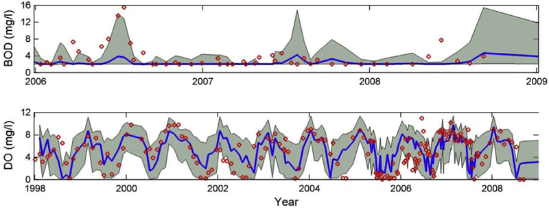
Observations (red dots) versus Bayesian averaged model predictions (blue line) plus 95% confidence bounds for BOD and Dissolved Oxygen. (For interpretation of the references to colour in this figure legend, the reader is referred to the Web version of this article.)

The results show that the Bayesian averaged model predictions capture the main trends and variations exhibited by the observations, and also that the computed confidence bounds enclose most of the observations. The existence of observations outside the 95% uncertainty bounds suggest that there may be processes not accounted for by the current model structure, parameters and forcing conditions. For example, there may be missing loads in the model inputs if there are unreported loads into the system. Or, there may be more complex model components such as a sediment digenesis model that are necessary to simulate with more accuracy the magnitude and seasonal variability of the benthic nutrient fluxes. The Sawgrass modeling results reflect the level of model skill typically observed in TMDL applications.

4.2.2. Nutrient TMDL and MOS

The unconditional distributions $f_{T{N}_{obs}|T{N}_{sim}}$ and $f_{T{P}_{obs}|T{P}_{\mathit{sim}}}$ were used to calculate the load reductions of TN and TP necessary to achieve the water quality goals in Sawgrass Lake. In particular, the maximum loads of TN and TP were computed to satisfy $P_{{\overline{TN}}_{obs}>1.25}=P({\overline{TN}}_{obs}>1.25mg/L\left|{(\overline{TN}}_{sim}\right|{\mathbf{\text{TN}}}_{\mathbf{\text{load}}})>1.25mg/L)\le \beta$ and $P_{{\overline{\mathit{TP}}}_{obs}>0.075}=P({\overline{TP}}_{obs}>0.075\mathit{\text{mg}}/L\left|{(\overline{TP}}_{\mathit{sim}}\right|{\mathbf{\text{TP}}}_{\mathbf{\text{load}}})>0.075\mathit{\text{mg}}/L)\le \beta$ where ${\overline{TN}}_{obs}$ and ${\overline{TP}}_{obs}$ are the annual geometric means of TN and TP, TN_load and TP_load are the unknown TMDL loads and β is the acceptable risk of non-compliance (β).

The strategy to obtain the loads TN_load and TP_load was as follows: First, the model was executed with different values of TN_load and TP_load by applying reduction factors to the input time series of N and P loads. Second, the unconditional distributions $f_{{\mathit{\text{TN}}}_{\mathit{\text{obs}}}|T{N}_{\mathit{\text{sim}}}}$ and $f_{T{P}_{\mathit{\text{obs}}}|T{P}_{\mathit{\text{sim}}}}$ were updated using TN_load and TP_load and the posterior probability distributions computed in Section 4.2.1. Third, the updated distributions $f_{{\mathit{\text{TN}}}_{\mathit{\text{obs}}}|T{N}_{\mathit{\text{sim}}}}$ and $f_{T{P}_{\mathit{\text{obs}}}|T{P}_{\mathit{\text{sim}}}}$ were used to compute the Bayesian average model predictions of TN and TP for the simulation period 1/1/1998 – 12/31/2008 and the results used to computed the geometric means ${\overline{TN}}_{sim}$ and ${\overline{TP}}_{sim}$. Finally, Eq. (24) was used to compute ${\overline{TN}}_{obs}$ and ${\overline{TP}}_{obs}$ using different values of β. Results of the above process are summarized in Fig. 11 for different load reduction scenarios ranging from 10% to 90% of the baseline loads of TN and TP and for the following risks of non-compliance: β = 10%, 30%, 50% 70% and 90%.

Fig. 11.

Expected ${\overline{\mathit{TP}}}_{obs}$ and ${\overline{TN}}_{obs}$ concentrations for different load reduction alternatives and risks of non compliance.

Fig. 11 shows how the computed load reductions of TN and TP vary as a function of β. In the particular case of TN, Fig. 11 indicates that in order to meet the nutrient concentration of TN ≤ 1.25 mg/L it is necessary to have a TN load reduction of at least 26% for a 10% risk of non-compliance, or a load reduction of at least 11% for a 90% risk of non-compliance. In the case of TP, Fig. 11 suggests that in order to meet the nutrient concentration of TP ≤ 0.075 mg/L it is necessary to reduce the current TP load in at least 37% for a 10% risk of non-compliance, or in at least 12% for a 90% risk of non-compliance. From these results, it is clear that the higher the risk of non-compliance β, the lower the load reduction necessary for the TMDL. And vice versa, the lower the risk of non-compliance, the larger the load reduction necessary. β is then an important parameter that should be defined based on economic and engineering feasibility studies, and between stakeholders and other parties involved in the definition and enforcement of the local environmental legislation.

For the particular requirements of the problem, the necessary load reductions to satisfy the annual geometric mean concentrations of TN = 1.25 mg/L and TP = 0.075 mg/L with a risk of non-compliance of β =30% were 25% reduction of TN and 31% reduction of TP. The margins of safety (MOS) associated with these load reductions were calculated using Eq. (25). To obtain the maximum allowable loads without an account for uncertainty (L in Eq. (25)), the calibrated model (Table 5) was executed with reduced loads of TN and TP until the geometric means of TN and TP satisfied the standard concentrations. The calculated load reductions were 17% for TN and 20% for TP. The MOS for TN and TP were then computed as the difference between the load reductions calculated with the calibrated model using the traditional approach and the load reductions calculated using the full uncertainty analysis. The resulting MOS were 8% for TN and 10% for TP.

5. Discussion and conclusions

This investigation presented a strategy to explicitly evaluate and incorporate uncertainty in the estimation of TMDLs and MOS. The most relevant aspects of this strategy include:

• It uses an improved equation (Eq. (3)) to calculate the TMDL risk of non-compliance which is defined as the probability that water quality observations will violate a particular standard once the TMDL is implemented (Appendix A). The TMDL is determined using Eq. (3) by calculating the risk of non-compliance of different load reduction alternatives and by selecting the maximum load that satisfies a predefined acceptable risk of non-compliance.

• The framework, as in other existing risk based approaches requires the definition of an acceptable risk of non-compliance β (e.g Borsuk et al., 2002; Chen et al., 2012; Hantush and Chaudhary, 2014).

• The new expression to compute the risk of non-compliance (Eq. (3)) allows an explicit assessment of parametric and model uncertainty in the TMDL process and provides a path to explicitly evaluate the MOS as was presented in Section 2. Eq. (3) also includes a new explicit mathematical expression to account for the conditionality between the observations and model predictions. When the equation is used, it provides an estimate of observable future water quality conditions conditional on the predictions of the model and taking into account model and parametric sources of uncertainty. The resulting approach is a formal strategy that is solved based on Monte Carlo analysis and Bayesian inference.

The formulation of a TMDL as a problem of risk of non-compliance has important advantages. The most evident is that this risk can be related more naturally to current water quality standards. For instance, for the state of Florida, the recently adopted nutrient criteria rule 62–302.531 issued on 2/17/2016, states that the annual geometric means of TN and TP should not be exceeded more than once in any consecutive three year period. This frequency can be translated into an acceptable frequency or risk of non-compliance of 1 in 3 or β = 33.33% which can be used to compute the necessary nutrient load reduction as illustrated in the Sawgrass Lake example. In the proposed framework the Margin of Safety (MOS) becomes a function of the risk of non-compliance, thus facilitating the comparison between different TMDL studies and results. The risk of non-compliance is the basis for a more objective and convenient approach to set the goals of the TMDL and to define the MOSs.

An additional advantage of defining an acceptable risk of non-compliance for the TMDL is that it is also possible to link this risk to a formal probabilistic expression to compute the TMDL. This investigation introduces the conditional probability given by Eq. (3) for this purpose. Eq. (3) represents the probability that once the TMDL for a target variable such as TN or TP is implemented, the actual water body concentrations will exceed a specific standard, given that the standard is exceeded by the model predictions. This equation can be used to calculate the TMDL if a specific risk of non-compliance is provided as illustrated for Sawgrass Lake. The conditional probability given by Eq. (3) also represents an expression of uncertainty, and thus, constitutes an objective approach to incorporate uncertainty in TMDL studies.

The conditional probability distribution shown in Eq. (3) is computed using the model conditional processor proposed by Todini (2008). This strategy is robust and relatively straightforward to implement but has a couple of limitations that must be taken into account during its implementation. The first limitation is that the selection of a probability model to fit the upper and lower tails of the observations, i.e. Eq. (12) and Eq. (13), can be very challenging, especially because water quality time series are generally short and discontinuous. Because the tail models fit in particular extreme probabilities, it is important to evaluate if the models in Eq. (12) and Eq. (13) are the best alternative to the problem at hand or if other alternative models can provide a better fit. The second challenge also resulting from the fact that water quality time series are short and discontinuous is that the correlation coefficient between observations and model predictions in the normal space can be very low and lead unrealistically to high levels of uncertainty, see Eq. (11). The above problems are challenges that require more research as of 2018, but it is reasonable to think that as methods to obtain water quality observations become cheaper and more portable, the limitations caused by short time series will be resolved.

The framework introduced in Section 2 also accounts for the impacts of parametric uncertainty by marginalizing the posterior parameter distribution from the conditional distribution using Eq. (16). The computation of the posterior parameter distribution relies on the use of the likelihood function recently proposed by Hantush and Chaudhary (2014) and follows the traditional Bayesian inference process (Dilks et al., 1992). Once computed, is possible to obtain the marginal distributions of the individual parameters and calibrated estimates using any central tendency measure such as the average or median of the distribution.

Finally, the Margin of Safety (MOS), which is an important aspect of a TMDL application can be obtained through Eq. (26) by computing the difference between the permissible load calculated using the uncertainty framework presented in Section 2, and the permissible load calculated as usual using the calibrated model. The rationale of Eq. (26) suggests in principle that the load computed using the traditional approach is close to the expected or most probable load reduction necessary to achieve the TMDL goals, and that the load computed using the proposed approach accounts for the confidence level necessary to achieve such goals taking into account the existence of different sources of uncertainty.

Fig. 9.

Observations (red dots) versus Bayesian averaged model predictions (blue line) plus 95% confidence bounds for TP, phosphorus subspecies and Chlorophyll a. (For interpretation of the references to colour in this figure legend, the reader is referred to the Web version of this article.)

Appendix A. Definition of risk in the context of Total Maximum Daily Load applications

Because the definition of risk can vary depending on the field of study and the strategies used for its calculation, it is necessary to provide an explicit definition of risk for TMDL studies. In engineering, risk is defined as the probability of failure of a system. This definition of risk is derived from the concept of performance failure which is used in engineering to describe a system that is unable to perform as expected. As described by Singh et al. (2007), a system fails when the demand, or loading D exceeds the capacity or resistance R of the system. The probability of failure or risk can be expressed in terms of D and R as

$$P_f=P\left(D>R\right)$$ (A.1)

The above concepts can be applied in the context of water quality. A TMDL reaches a point of performance failure when the receiving water body is unable to maintain the water quality below or above the levels defined by the water quality standards. For example, if a water quality standard defines a minimum concentration that must be maintained in the water body c*, the TMDL has a performance failure when the observed concentrations Z exceed c*. The probability of failure or risk can now be expressed in terms of Z and c* as

$$P_{f_{-}TMDL}=P\left(Z>c^{*}\right)$$ (A.2)

To directly evaluate $P\left(Z>c^{*}\right)$, the TMDL must be implemented and then the water quality concentrations Z monitored long enough to allow the adjustment of a probability distribution. This is obviously unrealistic as decision makers need to know $P\left(Z>c^{*}\right)$ prior to the TMDL implementation. To solve this issue, an approximation of $P\left(Z>c^{*}\right)$ can be obtained by using mathematical model predictions of the water quality concentrations under the TMDL. In particular, if the model predictions are denoted by Y, then Eq. (A.2) can be calculated as

$$P_{f_{-}TMDL}=P\left(Z>c^{*}|Y>c^{*}\right)$$ (A.3)

Equation (A.3) is solved following the procedures described in Section 2 and can be used in two ways. First to know the probability of failure P_{f_TMDL} of a TMDL if the TMDL is known, and second, to back calculate the TMDL if the probability of failure P_{f_TMDL} is known. The first application is a traditional problem where the demand or loading D and the capacity or resistance R of the system are known. The second application requires the definition of an allowable probability of failure. This probability can be directly obtained from the definition of a particular water quality standard, or by consensus between stakeholders and state agencies of water quality protection.

In practice, water quality standards have an acceptable frequency of “failure” of the TMDL. These are acute or sporadic events when the water quality is allowed to fall below the desired levels without causing a permanent damage to the ecological integrity of the water body. This frequency can be translated into a probability (β) (similar to the way the frequency of heads and tails outcomes of a coin toss is translated into probability) to back calculate the TMDL as proposed in this investigation. By using the probability β, the TMDL must satisfy P_{f_TMDL} < β or

$$P_{f_{-}TMDL}=P\left(Z>c^{*}|Y>c^{*}\right)<\beta$$ (A.4)

Appendix B. Practical implications of the use of Bayesian Analysis

For practitioners unfamiliar with Bayesian Analysis sometimes is difficult to identify the differences between a traditional calibration procedure and calibrations based on Bayesian Analysis. A brief discussion on the topic is presented below.

Traditionally, during a manual calibration or automatic calibration procedure, a model is executed several times with different parameter combinations. For each run, the goodness of fit is evaluated using statistics such as relative error, index of agreement, mean squared error, Nash and Sutcliffe criterion and hypothesis testing comparing means, variances etc between the model predictions and observations. The process is repeated until a desired level of model performance has been reached and ultimately leads to the calibrated set of parameter values.

The purpose of a Bayesian Monte Carlo analysis is not only to obtain the calibrated parameter values but to obtain the full probability distribution of the model parameters to be able to quantify the level of dispersion in the distributions and propagate it to the model predictions to determine the impacts of parametric uncertainty (Mantovan and Todini, 2006). The parameter distributions are obtained by means of Eq. (18). Once the parameter distributions are calculated, then it is possible to obtain the calibrated parameter values using any measure of central tendency of the distributions such as the median or mean. With the posterior parameter distribution it is also possible to obtain the 5% and 95% confidence bounds around the predictions of the calibrated model.

At the core of the Bayesian analysis lies the likelihood function which is a probability density function used to describe the statistical properties of the residuals between the model predictions and the observations. The residuals are usually biased, have trends and/or are correlated. These are some of the most critical statistical properties that must be captured while developing the likelihood function. The use of the likelihood function ensures that the Bayesian analysis will converge to the true parameter probability distributions (Bayesian consistency) if an infinite combinations of model parameter values are evaluated through Monte Carlo experiments (Bayesian coherence).

The likelihood function presented in this investigation is able to represent the bias and correlation of the residuals. In the theoretical example was demonstrated that by using this likelihood function the Bayesian analysis procedure was able to back calculate with high accuracy the parameter values used to generate the data. For more details on Bayesian analysis the reader is referred to Kennedy and O’Hagan (2001); Mantovan and Todini (2006) and Qian et al.(2003).

Appendix C. Calculation of the likelihood function $L(\mathbf{\text{θ}}|Z,\mathbf{X})$

The following first-order autoregressive error model is used by Hantush and Chaudhary (2014) and Li et al. (2011) to represent a sequence of errors that is biased and autocorrelated

$${\epsilon }_t-\mu =\varphi \left[{\epsilon }_{t-1}-\mu \right]+\epsilon$$ (C.1)

where μ is the mean of the residuals, ϕ is a first order correlation coefficient and $\epsilon ~N\left(0,{\sigma }_{\epsilon }^2\right)$. Note from the properties of autoregressive models that ϕ < 1 to satisfy stationarity. Further, note that because ε is Gaussian, ε is also Gaussian and follows the distribution $\epsilon ~N\left[\mu ,{\sigma }_{\epsilon }^2/\left(1-{\varphi }^2\right)\right]$. The likelihood function for this error model is given by,

$$L\left({\mathbf{\text{θ}}}_i\right)={(2\pi )}^{-n/2}{\left({\sigma }_{\epsilon i}\right)}^{-n}\prod _{j=1}^n\mathit{exp}\left\{-\frac{1}{2}{\left[\frac{{\epsilon }_j-{\mu }_i-{\varphi }_i\left({\epsilon }_{j-1}-{\mu }_i\right)}{{\sigma }_{\epsilon i}}\right]}^2\right\}$$ (C.2)

Eq. (C.2) is a conditional distribution and is valid for moderate to large sample sizes of n. Parameters of this error model (μ, ϕ and ${\sigma }_{\epsilon }^2$) can be estimated using Bayesian analysis, maximum likelihood, nonlinear least squares or any other approach. Bayesian analysis is probably the most common approach, but requires large amounts of Monte Carlo simulations to compute $\widehat{\mu }$, $\widehat{\varphi }$ and ${\widehat{\sigma }}_{\epsilon }^2$ and the parameters from the hydrologic or water quality model. To reduce the number of parameters for the inference process, Hantush and Chaudhary (2014) proposed the use of maximum likelihood, which, although it requires a considerable amount of algebraic operations, provides analytical estimates of $\widehat{\mu }$, $\widehat{\varphi }$ and ${\widehat{\sigma }}_{\epsilon }^2$. These estimates are computed first by equating the partial derivatives of the logarithm of Eq. (C.2) to zero with respect to each parameter and then by solving for the unknowns $\widehat{\mu }$, $\widehat{\varphi }$ and ${\widehat{\sigma }}_{\epsilon }^2$. This process leads to (Hantush and Chaudhary, 2014):

$${\widehat{\mu }}_i=\frac{1}{n\left(1-{\widehat{\varphi }}_i\right)}\sum _{j=1}^n\left({\epsilon }_j-{\widehat{\varphi }}_i{\epsilon }_{j-1}\right)$$ (C.3)

$${\widehat{\sigma }}_{{\epsilon }_i}^2=\frac{1}{n}\sum _{j=1}^n{\left[{\epsilon }_j-{\widehat{\mu }}_i-{\widehat{\varphi }}_i\left({\epsilon }_{j-1}-{\widehat{\mu }}_i\right)\right]}^2$$ (C.4)

and finally $\widehat{\varphi }$ is computed by solving the quadratic equation $A{\widehat{\varphi }}^2+B\widehat{\varphi }+C=0$

$${\widehat{\varphi }}_i=\frac{-B\pm \sqrt{B^2-4AC}}{2A}$$ (C.5)

where

$$\begin{gathered} A={\left(\sum _{j=1}^n{\epsilon }_{j-1}\right)}^2-n\sum _{j=1}^n{\left({\epsilon }_{j-1}\right)}^2 \\ B=n\sum _{j=1}^n{\left({\epsilon }_{j-1}\right)}^2-\sum _{j=1}^n{\epsilon }_{j-1}\left(\sum _{j=1}^n{\epsilon }_j+\sum _{j=1}^n{\epsilon }_{j-1}\right)+n\sum _{j=1}^n{\epsilon }_j{\epsilon }_{j-1} \\ C=\sum _{j=1}^n{\epsilon }_j\left(\sum _{j=1}^n{\epsilon }_{j-1}\right)-n\sum _{j=1}^n{\epsilon }_j{\epsilon }_{j-1} \end{gathered}$$ (C.6)

Note that for every parameter combination ${\mathbf{\text{θ}}}_i,i=1,2,\dots m$, of the hydrologic or water quality model, there exists a corresponding set of parameters ${\widehat{\mu }}_i,{\widehat{\varphi }}_i$ and ${\widehat{\sigma }}_{{\epsilon }_i}^2$ of the error model. To obtain the overall parameter estimates of the error model it is possible to compute a weighted average value based on the support of the posterior distribution $f_{\mathbf{\text{θ}}}(\mathbf{\text{θ}}|Z,\mathbf{X})$ by

$$\widehat{\mu }=\sum _{i=1}^m{\widehat{\mu }}_i{f}_{{\mathbf{\text{θ}}}_i}\left({\mathbf{\text{θ}}}_i|Z,\mathbf{X}\right)$$ (C.7)

$${\widehat{\sigma }}_{\epsilon }^2=\sum _{i=1}^m{\widehat{\sigma }}_{{\epsilon }_i}^2{f}_{{\mathbf{\text{θ}}}_i}\left({\mathbf{\text{θ}}}_i|Z,\mathbf{X}\right)$$ (C.8)

$$\widehat{\varphi }=\sum _{i=1}^m{\widehat{\varphi }}_i{f}_{{\mathbf{\text{θ}}}_i}\left({\mathbf{\text{θ}}}_i|Z,\mathbf{X}\right)$$ (C.9)

Appendix D. Estimation of Calibrated Parameters from the Posterior Parameter Distribution f_θ

Once $f_{\mathbf{\text{θ}}}(\mathbf{\text{θ}}|Z,\mathbf{X})$ has been computed (Section 2.2), it is easy to proceed with the computation of the marginal distributions of the water quality model parameters ${\theta }_1,{\theta }_2\dots {\theta }_p\text{i.e.}f\left({\theta }_1\right),f\left({\theta }_2\right)\dots f\left({\theta }_p\right)$ and to obtain single point estimates ${\widehat{\theta }}_1,{\widehat{\theta }}_2\dots {\widehat{\theta }}_p$. As an example, the general expression for the marginal distribution of the parameter θ_k i.e. f(θ_k) is given by

$$f\left({\theta }_k\right)=\underset{{\theta }_1\dots {\theta }_{k-1},{\theta }_{k+1}\dots {\theta }_p}{\int }{f}_{\mathbf{\text{θ}}}(\mathbf{\text{θ}}|\mathbf{Z},\mathbf{X})d{\theta }_1\dots d{\theta }_{k-1}d{\theta }_{k+1}\dots d{\theta }_p$$ (D.1)

or in discrete terms by,

$$f\left({\theta }_k\right)=\sum _{{\theta }_1\dots {\theta }_{k-1},{\theta }_{k+1}\dots {\theta }_p}{f}_{\mathbf{\text{θ}}}(\mathbf{\text{θ}}|\mathbf{Z},\mathbf{X})$$ (D.2)

and once obtained, it is possible to find the single point estimate of θ_k (i.e. ${\widehat{\theta }}_k$) by computing the mean or expected value of the distribution f(θ_k), which is mathematically equivalent to the first moment of area

$$f\left({\theta }_k\right)={\int }_d^e{\theta }_{k}f\left({\theta }_k\right)d{\theta }_k$$ (D.3)

or in discrete terms

$$f\left({\theta }_k\right)=\sum _{l=d}^e{\theta }_{k}f\left({\theta }_k\right)$$ (D.4)

where [d, e] represents the range of θ_k.

References

- Alameddine I, Cha Y, Reckhow KH, 2011. An evaluation of automated structure learning with Bayesian networks: an application to estuarine chlorophyll dynamics. Environ. Model. Software 26 (2), 163–172. [Google Scholar]
- Ambrose RB, Wool TA, Martin JL, 1993. The Water Quality Analysis Simulation Program, WASP5, Part a: Model Documentation. U.S. EPA Center for Exposure Assessment Modeling, Athens, GA. [Google Scholar]
- Ames DP, Lall U, 2008. Developing total maximum daily loads under uncertainty: decision analysis and the margin of safety. J. Contemp. Water Res. Educ. 140 (1), 37–52. [Google Scholar]
- Borsuk ME, Stow CA, Reckhow KH, 2002. Predicting the frequency of water quality standard Violations: a probabilistic approach for TMDL development. Environ. Sci. Technol. 36 (10), 2109–2115. [DOI] [PubMed] [Google Scholar]
- Camacho RA, Martin JL, McAnally W, Díaz-Ramirez J, Rodriguez H, Sucsy P, Zhang S, 2015. A comparison of bayesian methods for uncertainty analysis in hydraulic and hydrodynamic modeling. JAWRA J. Am. Water Res. Assoc. 51 (5), 1372–1393. [Google Scholar]
- Camacho RA, Martin JL, Watson B, Paul MJ, Zheng L, Stribling JB, 2014. Modeling the factors controlling phytoplankton in the St. Louis bay estuary, Mississippi and evaluating estuarine responses to nutrient load modifications. J. Environ. Eng. 141 (3), 04014067. [Google Scholar]
- Chapra S, 1997. Surface Water - Quality Modeling. Waveland Press, Long Grove, Illinois. [Google Scholar]
- Chen D, Dahlgren RA, Shen Y, Lu J, 2012. A Bayesian approach for calculating variable total maximum daily loads and uncertainty assessment. Sci. Total Environ. 430, 59–67. [DOI] [PubMed] [Google Scholar]
- Cho E, Arhonditsis GB, Khim J, Chung S, Heo T-Y, 2016. Modeling metal-sediment interaction processes: parameter sensitivity assessment and uncertainty analysis. Environ. Model. Software 80, 159–174. [Google Scholar]
- Coccia G, Todini E, 2011. Recent developments in predictive uncertainty assessment based on the model conditional processor approach. Hydrol. Earth Syst. Sci. 15 (6), 3253–3274. [Google Scholar]
- Crumpacker AL, Butkus S, 2009. Approaches to defining TMDL margins of safety. Proc. Water Environ. Federation 2009 (6), 122–136. [Google Scholar]
- Dilks DW, Canale RP, Meier PG, 1992. Development of Bayesian Monte Carlo techniques for water quality model uncertainty. Ecol. Model. 62, 149–162. [Google Scholar]
- Dilks DW, Freedman PL, 2004. Improved consideration of the margin of safety in total maximum daily load development. J. Environ. Eng. 130 (6), 690–694. [Google Scholar]
- Franceschini S, Tsai CW, 2008. Incorporating reliability into the definition of the margin of safety in total maximum daily load calculations. J. Water Resour. Plann. Manag. 134 (1), 34–44. [Google Scholar]
- Gelman A, Carlin JB, Stern HS, Rubin DB, 2004. Bayesian Data Analysis. Chapman and Hall/CRC, Boca Raton, Fla. [Google Scholar]
- Gilks WR, Richardson S, Spiegelhalter DJ, 1996. Markov Chain Monte Carlo in Practice. Chapman and Hall, London. [Google Scholar]
- Gronewold AD, Borsuk ME, 2009. A software tool for translating deterministic model results into probabilistic assessments of water quality standard compliance. Environ. Model. Software 24 (10), 1257–1262. [Google Scholar]
- Hantush M, Chaudhary A, 2014. Bayesian framework for water quality model uncertainty estimation and risk management. J. Hydrol. Eng. 19 (9), 04014015. [Google Scholar]
- Kennedy MC, O’Hagan A, 2001. Bayesian calibration of computer models. J. Roy. Stat. Soc. Series B (Statistical Methodology) 63 (3), 425–464. [Google Scholar]
- Krzysztofowicz R, 1999. Bayesian theory of probabilistic forecasting via deterministic hydrologic model. Water Resour. Res. 35 (9), 2739–2750. [Google Scholar]
- Krzysztofowicz R, Kelly KS, 2000. Hydrologic uncertainty processor for probabilistic river stage forecasting. Water Resour. Res. 36 (11), 3265–3277. [Google Scholar]
- Kunz RG, 2011. Environmental Calculations: a Multimedia Approach. John Wiley and Sons. [Google Scholar]
- Langseth DE, Brown N, 2010. Risk-based margins of safety for phosphorus TMDLs in lakes. J. Water Resour. Plann. Manag. 137 (3), 276–283. [Google Scholar]
- Li L, Xu CY, Xia J, Engeland K, Reggiani P, 2011. Uncertainty estimates by Bayesian method with likelihood of AR (1) plus Normal model and AR (1) plus Multi-Normal model in different time-scales hydrological models. J. Hydrol. 406 (1–2), 54–65. [Google Scholar]
- Liang S, Jia H, Xu C, Xu T, Melching C, 2016. A Bayesian approach for evaluation of the effect of water quality model parameter uncertainty on TMDLs: a case study of Miyun Reservoir. Sci. Total Environ. 560–561, 44–54. [DOI] [PubMed] [Google Scholar]
- Mantovan P, Todini E, 2006. Hydrological forecasting uncertainty assessment: incoherence of the GLUE methodology. J. Hydrol. 330 (1–2), 368–381. [Google Scholar]
- Mara TA, Delay F, Lehmann F, Younes A, 2016. A comparison of two Bayesian approaches for uncertainty quantification. Environ. Model. Software 82, 21–30. [Google Scholar]
- Maranzano CJ, Krzysztofowicz R, 2004. Identification of likelihood and prior dependence structures for hydrologic uncertainty processor. J. Hydrol. 290 (1–2), 1–21. [Google Scholar]
- Martin JL, McCutcheon SC, 1999. Hydrodynamics and Transport for Water Quality Modeling. CRC Press, Boca Raton, FL. [Google Scholar]
- NRC, 2001. Assessing the TMDL Approach to Water Quality Management National Research Council Water Science and Technology Board, Division of Earth and Life Studies, Washington, D.C. [Google Scholar]
- Park D, Roesner LA, 2012. Evaluation of pollutant loads from stormwater BMPs to receiving water using load frequency curves with uncertainty analysis. Water Res. 46 (20), 6881–6890. [DOI] [PubMed] [Google Scholar]
- Patil A, Deng Z-Q, 2011. Bayesian approach to estimating margin of safety for total maximum daily load development. J. Environ. Manag. 92 (3), 910–918. [DOI] [PubMed] [Google Scholar]
- Qian SS, Stow CA, Borsuk ME, 2003. On Monte Carlo methods for bayesian inference. Ecol. Model. 159, 269–277. [Google Scholar]
- Reckhow KH, 2003. On the need for uncertainty assessment in TMDL modeling and implementation. J. Water Resour. Plann. Manag. 129, 245–246. [Google Scholar]
- Schoups G, Vrugt JA, 2010. A formal likelihood function for parameter and predictive inference of hydrologic models with correlated, heteroscedastic, and non-Gaussian errors. Water Resour. Res. 46 (10), W10531. [Google Scholar]
- Shirmohammadi A, Chaubey I, Harmel RD, Bosch DD, Munoz-Carpena R, Dharmasri C, Sexton A, Arabi M, Wolfe ML, Frankenberger J, Graff C, Sohrabi TM, 2006. Uncertainty in TMDL models. Transac. ASABE 49 (4), 1033–1049. [Google Scholar]
- Singh VP, Jain SK, Tyagi A, 2007. Risk and Reliability Analysis. ASCE press, Reston, VA. [Google Scholar]
- Thomann RV, Fitzpatrick JJ, 1982. Calibration and Verification of a Mathematical Model of the Eutrophication of the Potomac Estuary. Prepared for Department of Environmental Services. Government of the District of Columbia, Washington, D.C. [Google Scholar]
- Todini E, 2008. A model conditional processor to assess predictive uncertainty in flood forecasting. Int. J. River Basin Manag. 6 (2), 123–137. [Google Scholar]
- Todini E, 2009. Predictive uncertainty assessment in real time flood forecasting In: Baveye P, Laba M, Mysiak J (Eds.), Uncertainties in Environmental Modelling and Consequences for Policy Making. Springer Netherlands, pp. 205–228. [Google Scholar]
- U.S. Environmental Protection Agency, 1991. Guidance for Water Quality-based Decisions: the TMDL Process. Washington, D.C. [Google Scholar]
- U.S. Environmental Protection Agency, 1999. Protocol for Developing Nutrient TMDLs. Washington, D.C, p. 135. [Google Scholar]
- U.S. Environmental Protection Agency, 2009. Proposed Total Maximum Daily Loads for the Sawgras Lake WBID 28931 Nutrients and Dissolved Oxygen. Region 4, p. 33. [Google Scholar]
- Van der Waerden BL, 1952. Order tests for two-sample problem and their power I. Indagat. Math. 14, 453–458. [Google Scholar]
- Van der Waerden BL, 1953. Order tests for two-sample problem and their power II. Indagat. Math. 15, 303–310. [Google Scholar]
- Walpole RE, Myers RH, Myers SL, Ye KE, 2013. Probability and Statistics for Engineers and Scientists: Pearson New International Edition. Pearson Education Limited. [Google Scholar]
- Wool TA, Davie SR, Rodriguez HN, 2003. Development of three-dimensional hydrodynamic and water quality models to support TMDL decision process for the Neuse River estuary, North Carolina. J. J. Water Resour. Plann. Manag. 129, 295–306. [Google Scholar]
- Zhang HX, Yu SL, 2004. Appliying the first-order error analysis in determining the marging of safety for total maximum daily load computations. J. Environ. Eng. 130 (6), 664–673. [Google Scholar]
- Zou R, Carter S, Shoemaker L, Parker A, Henry T, 2006. Integrated hydrodynamic and water quality modeling system to support nutrient total maximum daily load development for Wissahickon Creek, Pennsylvania. J. Environ. Eng. 132 (4), 555–566. [Google Scholar]