Audiovisual detection at different intensities and delays

Abstract

In the redundant signals task, two target stimuli are associated with the same response. If both targets are presented together, redundancy gains are observed, as compared with single-target presentation. Different models explain these redundancy gains, including race and coactivation models (e.g., the Wiener diffusion superposition model, Schwarz, 1994, Journal of Mathematical Psychology, and the Ornstein Uhlenbeck diffusion superposition model, Diederich, 1995, Journal of Mathematical Psychology). In the present study, two monkeys performed a simple detection task with auditory, visual and audiovisual stimuli of different intensities and onset asynchronies. In its basic form, a Wiener diffusion superposition model provided only a poor description of the observed data, especially of the detection rate (i.e., accuracy or hit rate) for low stimulus intensity. We expanded the model in two ways, by (A) adding a temporal deadline, that is, restricting the evidence accumulation process to a stopping time, and (B) adding a second “nogo” barrier representing target absence. We present closed-form solutions for the mean absorption times and absorption probabilities for a Wiener diffusion process with a drift towards a single barrier in the presence of a temporal deadline (A), and numerically improved solutions for the two-barrier model (B). The best description of the data was obtained from the deadline model and substantially outperformed the two-barrier approach.

Background

Integrating information from different senses improves perception and action, speeds up response time (RT), enhances detection and discrimination accuracy, and facilitates goal-directed arm movements (Cluff, Crevecoeur, & Scott, 2015; Crevecoeur, Munoz, & Scott, 2016; Diederich & Colonius, 2004b; Miller, 1982, 1986; Nickerson, 1973; Sakata, Yamamori, & Sakurai, 2004; Seilheimer, Rosenberg, & Angelaki, 2014; Stein & Stanford, 2008; Van Atteveldt, Murray, Thut, & Schroeder, 2014). Despite this extensive research, many questions about how the behavioral benefits of multisensory integration emerge remain unanswered (Chandrasekaran, 2017; Cluff et al., 2015; Crevecoeur et al., 2016).

The goal of this study was to further describe and understand how the behavioral benefits of multisensory integration on detection rate (i.e., accuracy or alternatively hit rate) and RT in two monkeys during simple detection of redundant audiovisual signals depend on both the intensity as well as the stimulus onset asynchrony (SOA). Several past studies have investigated how behavioral benefits of multisensory integration depend on intensity, SOA or the combination of the two (Crevecoeur et al., 2016; Diederich & Colonius, 2004b; Dixon & Spitz, 1980; Holmes, 2009; Stein, Meredith, Huneycutt, & McDade, 1989; Todd, 1912; van Wassenhove, Grant, & Poeppel, 2007). The typical pattern observed when studies manipulate sensory intensity is that multisensory benefits increase as sensory intensities decrease. This phenomenon is termed “inverse effectiveness” and is considered a hallmark of multisensory integration (Stein & Stanford, 2008). Similarly, SOA manipulations also exert effects on behavioral benefits. When sensory intensities are matched, maximal multisensory benefits are observed when the sensory cues occur near simultaneously, that is in “physiological synchrony” (Hershenson, 1962; Meredith, Nemitz, & Stein, 1987). When both intensity and SOA are manipulated, the interaction between these factors is often nonlinear and complex (Diederich & Colonius, 2004a). For instance, strong stimuli are integrated only when presented in near-synchrony, whereas for weaker stimuli, the time window of integration is larger (Diederich & Colonius, 2004b).

The majority of the studies described above focused on describing the behavioral benefits and rarely used formal models of multisensory integration to describe the behavior. A few studies have addressed this gap and modeled multisensory benefits depending on both sensory intensity and SOA (e.g., Diederich, 1995; Gondan, Götze, & Greenlee, 2010). These studies used the redundant signals task, in which participants are asked to respond in the same way to stimuli of different sources. If both stimuli are presented at the same time or with small stimulus onset asynchrony (SOA), redundancy gains are observed that typically exceed those from probability summation of the inputs (Miller, 1982, 1986). Because accuracy was at ceiling in most conditions, the studies by Diederich (1995) and Gondan et al. (2010) mainly focused on response time and placed relatively less emphasis on accuracy.

As a starting point to describe both the accuracy and RTs in a redundant signals task, we used the Wiener diffusion superposition model (Schwarz, 1989, 1994) that assumes additivity of visual and auditory inputs and accumulation to a bound (“absorbing barrier”). As currently implemented, the model assumes that evidence accumulation continues for infinite time (Figure 1A). For the Wiener process drifting to a single absorbing barrier, this implies that the observer will always detect the stimulus. Thereby, the model provides an approximate description of the RTs in many experiments, but it cannot account for detection accuracy, which was non-perfect for the two monkeys in the present study.

Figure 1. A schematic of the three models considered in the study.

A One barrier Wiener diffusion superposition model (DSM), with an upper bound at $u$. This model has been used to describe response times in multisensory detection tasks (Schwarz, 1994). B Extension of Model A with a temporal deadline. C Two-barrier Wiener diffusion model with asymmetric bounds at $u$ and $-\ell$. X-axes in all graphs show time. Y-axes the activation of the decision-variable. Solid blue line shows the accumulated drift at each time point (without the noise). At time t=τ, the drift rate and the diffusion noise change to highlight the piecewise homogenous nature of these Wiener diffusion models. For all simulations, at all time points, the diffusion noise variance was set to 4.3², drift rate was 0.03 and 0.14 for before and after τ. τ was set to be 800 ms for schematic purposes. Upper barrier for the A, B were set at 200. The lower barrier ($-\ell$) was set at −300.

We extended the basic model in two ways: In most experiments, there is a finite window to respond to a sensory input or participants may internally choose to restrict their decision process to a time interval (Figure 1B). In line with this notion, some response time models for simple responses and choice tasks assume an internal deadline (“fixed stopping time”) for accumulation of sensory evidence (Busemeyer & Diederich, 2002; Diederich, 2008; Diederich & Oswald, 2016; Ratcliff, 2006; Ratcliff & Rouder, 2000; Ruthruff, 1996; Swensson, 1972). After the deadline, the response is omitted, or a guess is made (Yellott, 1971). We hypothesized that the incorporation of such a response deadline could explain both the RTs and accuracy of observers performing multisensory detection tasks. We, therefore, expanded on the single-barrier Wiener diffusion superposition model by incorporating a deadline for accumulation, and we derived closed-form expressions for the mean latencies and the probability of responses to synchronous and asynchronous stimuli in such a deadline model (Appendix A).

As a second extension, we adopted a second absorbing barrier representing omitted responses (Figure 1C, “nogo” barrier, see Gomez, Ratcliff, & Perea, 2007). This extension results in a two-barrier model, similar to Ratcliff’s diffusion decision model for two alternatives (Ratcliff, 1978; Ratcliff & McKoon, 2008). In this architecture, sensory evidence is accumulated until one of two absorbing barriers is reached: if the positive barrier is reached first, a response is initiated; whereas if the negative barrier is reached first, the response is withheld. Two-barrier diffusion models have been used to describe response times and accuracy in many two-choice tasks (Laming, 1968; Palmer, Huk, & Shadlen, 2005; Ratcliff & McKoon, 2008; Ratcliff, Smith, Brown, & McKoon, 2016; Ratcliff, Thapar, & McKoon, 2003; Smith & Ratcliff, 2004), Go-/Nogo tasks (Gomez et al., 2007), and in a redundant signals task with two alternatives (Blurton, Greenlee, & Gondan, 2014).

In the present study, Monkeys detected visual, auditory, and audiovisual vocalizations with delays between the stimulus components (Miller, 1986) in a background of noise (Chandrasekaran, Lemus, & Ghazanfar, 2013; Chandrasekaran, Lemus, Trubanova, Gondan, & Ghazanfar, 2011). The behavioral benefits accrued by monkeys when detecting audiovisual stimuli are a systematic function of both the intensities and the delay between sensory stimuli (Ulrich & Miller, 1997). We tested the three models, the basic single barrier Wiener diffusion model (Schwarz, 1989, 1994), a single barrier Wiener diffusion model with a temporal deadline, and the two-barrier Wiener diffusion model, using the mean RTs and hit rates of two monkeys performing the detection task at different signal to noise ratios (SNRs) and SOAs. It turned out that the expansion of the diffusion superposition model with a deadline greatly improved the model fit. In contrast, a two-barrier model (Gomez et al., 2007) performed rather poorly.

The manuscript is organized as follows. We first provide a compact summary of the redundant signals detection task and the Wiener diffusion superposition model, as implemented by Schwarz (1994). We then describe the detection task used in monkeys and show that the simple model fits poorly to the accuracy and response times. Our contribution is to show that extending the model by incorporating a deadline for accumulation provides a better account of the observed behavior compared to the two-barrier Wiener diffusion model.

Redundant signals task

The redundant signals task is a simple and powerful experimental paradigm for investigating multisensory perception. In this task, subjects are asked to respond in the same way to stimuli of two sensory modalities, for example, auditory and visual stimuli (A, V, Hershenson, 1962; Todd, 1912). The typical finding is that if signals from both modalities are present (redundant signals, AV), average responses are faster than from any single sensory modality (Diederich & Colonius, 2004a; Miller, 1982, 1986; Raab, 1962).

Such redundant signals effects, by themselves, are not necessarily indicative of any special mechanism that integrates the information of the different channels. For example, redundancy gains may arise from a race between the channel-specific detection processes (“race model,” Miller, 1982; Raab, 1962) for redundant stimuli but not in the single stimuli. When two racers are present, the slowest response times are removed and thus the mean response time is faster. In audiovisual detection tasks, however, redundancy gains are typically larger than predicted by race models. These redundancy gains are thought to be better explained by “coactivation models” that assume some integration of the information provided by the two sensory systems (Diederich, 1995; Diederich & Colonius, 2004b; Miller, 1986, Eq.3; Schwarz, 1989, 1994). One such model is the Wiener diffusion superposition model, which we summarize below (see also Figure 1).

Wiener diffusion superposition model

The Wiener diffusion superposition model is a coactivation model that describes redundancy gains assuming additive superposition of channel-specific Wiener diffusion processes (Schwarz, 1994; see Diederich, 1992, 1995, for a model with superposition of Ornstein-Uhlenbeck processes). Schwarz’s model assumes that the presentation of a stimulus leads to a buildup of evidence that is described by a Wiener diffusion process $\mathbf{X}\left(t\right)$ with drift $\mu$ and variance ${\sigma }^2>0$ (Ratcliff, 1978; Ratcliff & McKoon, 2008; Ratcliff et al., 2016; Smith & Ratcliff, 2004). In a model with a single criterion (“absorbing barrier”), the stimulus is ‘detected’ when an evidence criterion $c>0$ is met for the first time. The density $f_{\text{IG}}\left(t\right)$ and the distribution $F_{\text{IG}}\left(t\right)$ of the first-passage times $\mathbf{D}$ are then inverse Gaussian (Cox & Miller, 1965),

$$f_{\text{IG}}\left(t|c,\mu ,{\sigma }^2\right)=\frac{c}{\sqrt{2\pi {\sigma }^2{t}^3}}\cdot \text{exp}\left(-\frac{{\left(c-\mu t\right)}^2}{2{\sigma }^{2}t}\right)$$ (1)

$$F_{\text{IG}}\left(t\text{ | }c,\mu ,{\sigma }^2\right)=\text{Φ}\left(\mu t\text{ | }c,{\sigma }^{2}t\right)+\text{exp}\left(\frac{2c\mu }{{\sigma }^2}\right)\text{Φ}\left(-\mu t\text{ | }c,{\sigma }^{2}t\right)$$ (2)

with $\text{Φ}\left(x \text{|} m,s^2\right)$ denoting the Normal distribution function with mean $m$ and variance $s^2$. The expected detection time $E\left(\mathbf{D}\right)$ is obtained by ${\int }_0^{\infty }t\cdot f_{\text{IG}}\left(t \text{|} c, \mu ,{\sigma }^2\right)\hspace{0.17em}dt$, which simplifies to

$$E\left(\mathbf{D}\right)=c/\mu$$ (3)

Predictions for the detection times for unimodal stimuli A and V are, therefore, easily obtained, $c/{\mu }_{\text{A}}$ and $c/{\mu }_{\text{V}}$, respectively. When two stimuli are presented simultaneously, coactivation occurs. The model assumes that the two modality-specific processes superimpose linearly, ${\mathbf{X}}_{\text{AV}}\left(t\right)={\mathbf{X}}_{\text{A}}\left(t\right)+{\mathbf{X}}_{\text{V}}\left(t\right)$. The new process ${\mathbf{X}}_{\text{AV}}$ is again a Wiener diffusion process with drift ${\mu }_{\text{AV}}={\mu }_{\text{A}}+{\mu }_{\text{V}}$ and variance ${\sigma }_{\text{AV}}^2={\sigma }_{\text{A}}^2+{\sigma }_{\text{V}}^2+2{\rho }_{\text{AV}}{\sigma }_{\text{A}}{\sigma }_{\text{V}}$ (under the assumption that ${\mathbf{X}}_{\text{A}}$ and ${\mathbf{X}}_{\text{V}}$ are uncorrelated, the covariance term is zero). Since the drift parameters add up, ${\mathbf{X}}_{\text{AV}}$ reaches the response criterion earlier than any of its single constituents, resulting in faster responses to redundant stimuli,

$$E\left({\mathbf{D}}_{\text{AV}}\right)=\text{c}/\left({\mu }_{\text{A}}+{\mu }_{\text{V}}\right)$$

What happens in stimuli presented with onset asynchrony (SOA, e.g., V100A, i.e., V is presented at $t=0$, and A follows $\tau =100$ ms later)? During the first $\tau$ ms, sensory evidence is accumulated by the visual channel alone. If the criterion is reached within this interval, the stimulus is detected, and a response is initiated. This happens with probability $P\left({\mathbf{D}}_{\text{V}\left(\tau \right)\text{A}}\le \tau \right)=F_{\text{IG}}\left(\tau |c,{\mu }_{\text{V}},{\sigma }_{\text{V}}^2\right)$ given by Equation 2.

On average, this occurs within

$$E\left({\mathbf{D}}_{\text{V}\left(\tau \right)\text{A}}|{\mathbf{D}}_{\text{V}\left(\tau \right)\text{A}}\le \tau \right)=\frac{1}{P\left({\mathbf{D}}_{\text{V}\left(\tau \right)\text{A}}\le \tau \right)} {\int }_0^{\tau }t\cdot f_{\text{IG}}\left(t|c,{\mu }_{\text{V}},{\sigma }_{\text{V}}^2\right) dt$$ (4)

The solution for the integral is given by Schwarz (1994, Eq. 6). In the other case, the process has attained a subthreshold activation level $\mathbf{X}\left(\tau \right)=x<c$, with density described by

$$w_{\text{IG}}\left(x,\tau |c,{\mu }_{\text{V}},{\sigma }_{\text{V}}^2\right)=\varphi \left(x|{\mu }_{\text{V}}\tau ,{\sigma }_{\text{V}}^2\tau \right)-\text{exp}\left(\frac{2c{\mu }_{\text{V}}}{{\sigma }_{\text{V}}^2}\right)\cdot \varphi \left(x|2c+{\mu }_{\text{V}}\tau ,{\sigma }_{\text{V}}^2\tau \right),$$ (5)

(e.g., Schwarz, 1994, Eq. 7), and $\varphi$ denoting the Normal density. Because activation $x$ has already been attained at time $\tau$, the remaining activation needed to achieve the criterion is $c-x$. After time $\tau$, both channels accumulate evidence, resulting in a process drifting with ${\mu }_{\text{AV}}$:

$$E\left({\mathbf{D}}_{\text{V}\left(\tau \right)\text{A}}|\mathbf{X}\left(\tau \right)=x\right)=\tau +\frac{c-x}{{\mu }_{\text{AV}}}$$ (6)

This expectation must be integrated for all possible levels of activation $x<c$, weighted by the density (5) that level $x$ has been reached by time $t=\tau$:

$$E\left({\mathbf{D}}_{\text{V}\left(\tau \right)\text{A}}|{\mathbf{D}}_{\text{V}\left(\tau \right)\text{A}}>\tau \right)={\int }_{-\infty }^c{w}_{\text{IG}}\left(x,\tau |c,{\mu }_{\text{V}},{\sigma }_{\text{V}}^2\right)\cdot E\left({\mathbf{D}}_{\text{V}\left(\tau \right)\text{A}}|\mathbf{X}\left(\tau \right)=x\right)\hspace{0.17em}dx$$ (7)

An analytic solution for the expectation of ${\mathbf{D}}_{\text{V}\left(\tau \right)\text{A}}$ is given in Schwarz (1994, Eq. 10).

The diffusion process only describes the ‘detection’ latency $\mathbf{D}$, or processing time. To derive a prediction for the observed response time $\mathbf{T}$, an additional variable $\mathbf{M}$ is typically introduced that summarizes everything not described by the diffusion process (e.g., motor execution), such that $\mathbf{T}=\mathbf{D}+\mathbf{M}$. Therefore, the prediction for the mean response time is

$$E\left(\mathbf{T}\right)=E\left(\mathbf{D}\right)+{\mu }_{\text{M}}$$ (8)

Where the additional parameter denotes the expectation of $\mathbf{M}$. Schwarz (1994) demonstrated that such a model of additive superposition quite accurately describes the RTs reported for Participant B.D. from Miller (1986) in a speeded response task with 13 different SOAs.

The present experiment

We trained monkeys to detect visual, auditory and audiovisual vocal signals in a constant background of auditory noise (Chandrasekaran et al., 2011). We chose a free response paradigm (without explicit trial markers, Egan, Greenberg, & Schulman, 1961; Shub & Richards, 2009) because it mimics natural audiovisual communication—faces are usually continuously visible and move during vocal production. The task was a typical redundant signals task (Miller, 1982, 1986). The stimuli were chosen to approximate natural face-to-face vocal communication. The task of the monkeys was to detect the visual motion of the mouth of an avatar making a coo vocalization or the onset of the auditory component of a coo vocalization. Audiovisual stimuli were presented either in synchrony or at ten different SOAs.

Methods

Subjects

Nonhuman primate subjects were two adult male macaques (1 and 2, Macaca fascicularis). The monkeys were born in captivity and housed socially. The monkeys underwent sterile surgery for the implantation of a painless head restraint (see Chandrasekaran, Turesson, Brown, & Ghazanfar, 2010). All experiments and surgical procedures were performed in compliance with the guidelines of the Princeton University Institutional Animal Care and Use Committee.

Procedure

Experiments were conducted in a sound attenuating radio frequency enclosure. The monkey sat in a primate chair fixed 74 cm opposite a 19-inch CRT color monitor with a 1280 × 1024 screen resolution and 75 Hz refresh rate. The screen subtended a visual angle of 25° horizontally and 20° vertically. All stimuli were centrally located on the screen and occupied a total area (including blank regions) of 640 × 653 pixels. For every session, the monkeys were placed in a restraint chair and head-posted. A depressible lever (ENV-610M, Med Associates) was located at the center-front of the chair. Both monkeys spontaneously used their left hand for responses. Presentation (Neurobehavioral Systems) was used for stimulus presentation and data collection.

Stimuli

The stimuli for the behavioral task were inspired by the observation that besides providing benefits for discrimination of speech sounds (Besle, Fort, Delpuech, & Giard, 2004; Grant, Walden, & Seitz, 1998), visual speech enhances the detection of auditory speech (Grant, 2001; Grant & Seitz, 2000; Schwartz, Berthommier, & Savariaux, 2004). In such settings, the vocal components of the communication signals are degraded by environmental noise. The motion of the face, on the other hand, is usually perceived clearly. In the task, monkeys detected the onset of ‘coo’ calls. These coo calls are affiliative vocalizations commonly produced by macaque monkeys in a variety of contexts (Hauser & Marler, 1993; Rowell & Hinde, 1962).

Auditory Stimuli:

We used coo calls from two macaques as the auditory components of vocalizations; these were recorded from individuals that were unknown to the monkey subjects. Vocalizations could be one of three levels of sound intensity (85 dB, 68 dB, 53 dB) and were embedded in a constant background noise of 63 dB SPL. We therefore had auditory stimuli at three signal to noise ratios, SNRs, of High: +22 dB, Medium: +5 dB and low: –10 dB The vocalizations were resized to a constant duration of 400 ms using a phase vocoder (Flanagan & Golden, 1966) and normalized in amplitude (Figure 2A).

Figure 2. Stimuli and task structure for experiments in monkeys.

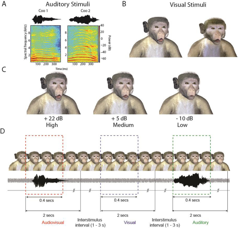
A: Waveform and spectrogram of coo vocalizations detected by the monkeys. B: Frames of the two monkey avatars at the point of maximal mouth opening for the largest SNR. C: Frames with maximal mouth opening from one of the monkey avatars for three different SNRs of +22 dB (High), +5 dB (Medium) and –10 dB (Low). D: Task structure for monkeys. An avatar face was always on the screen. Visual, auditory and audiovisual stimuli were randomly presented with an inter stimulus interval of 1–3 seconds drawn from a shifted and truncated exponential distribution. Responses within a 2 sec window after stimulus onset were considered hits. Responses in the inter-stimulus interval were considered to be response errors and led to timeouts.

Visual Stimuli.

The visual components of the vocalizations were 400 ms long videos of synthetic monkey agents making a coo vocalization. The size of the mouth opening was in accordance with the intensity of the associated vocalization: greater sound intensity was coupled to larger mouth openings by the dynamic face. For the three auditory SNRs, we had three corresponding mouth opening sizes. The animated stimuli were generated using 3D Studio Max 8 (Autodesk) and Poser Pro (Smith Micro), and were extensively modified from a stock model made available by DAZ Productions (Silver key 3D monkey, Figures. 2B, C). Further details of the generation of these visual avatars are available in a prior study (Chandrasekaran et al., 2011).

Audiovisual Stimuli.

The audiovisual stimuli were generated by presenting both the visual and auditory components either in synchrony or at 10 different SOAs. Audition could precede vision by 240, 160, 120, 80 or 40 ms and vice versa. For audiovisual stimuli the intensities were always paired; that is, the weak auditory stimulus was always paired with a small mouth opening (A_highV_high, A_mediumV_medium, A_lowV_low). We, therefore, had 3 matched audiovisual intensities and 11 asynchronies (10 SOA plus synchrony), which resulted in 33 AV conditions in total. Each block also had 3 auditory intensities and 3 visual intensities. Catch trials (C) were used to discourage from spontaneous responses and to control for fast guesses in the RT analysis (Eriksen, 1988).

Task

During the task (Figure 2D), an avatar face (e.g., Avatar 1) was continuously present on the screen; the background noise was also continuous. In the visual-only condition (V), Avatar 1 moved its mouth without any corresponding auditory component. In the auditory-only condition (A), the vocalization paired with Avatar 2 was presented with the static face of Avatar 1. Finally, in the audiovisual condition (AV), Avatar 1 moved its mouth accompanied by the corresponding vocalization of Avatar 1 and in accordance with its intensity. We, therefore, had two AV stimuli (A1V1 and A2V2). In the even blocks, the avatar face was the still frame of V1, A2 was the auditory sound played, and A1V1 was the audiovisual stimulus. The other block had the opposite configuration. This task design avoids the conflict between hearing a vocalization with the corresponding avatar face not moving (Fournier & Eriksen, 1990).

Stimuli of each condition (V, A, AV, C) were presented after a variable inter stimulus interval between 1 and 3 seconds (drawn from a shifted and truncated exponential distribution). Monkeys indicated the detection of a V, A or AV event by pressing the lever within 2 seconds following the onset of the stimulus. In the case of hits, the ISI was started immediately following a juice reward. In the case of misses, the ISI began after the two second response window.

After every block of 126 trials (33 AV stimuli + 3 A, 3 V, 3 catch stimuli, each stimulus condition repeated 3 times), a brief pause (~10 to 12 seconds) was imposed. Then, a new block was started in which, the avatar face, and the identity of the coo sound used for the auditory stimuli was switched. Within a block, all the conditions were randomly interleaved with one another.

In the behavioral dataset we analyzed here, we pooled the data across sessions. We analyzed 7477 trials from Monkey 1 and 8969 trials from Monkey 2, including hits and misses. We had approximately 191 trials per condition for Monkey 1 and about 229 trials per condition for Monkey 2.

Training

Monkeys were initially trained over many sessions to detect the coo vocalization events in visual, auditory or audiovisual conditions while withholding responses when no stimuli were presented. A press of the lever within a window starting 150 ms after onset of the vocalization event and within two seconds led to a juice reward and was defined as a hit. An omitted response in this two-second window was classified as a miss similar to the studies of free response tasks (without explicit trial markers , Egan et al., 1961; Shub & Richards, 2009). Lever presses to catch trials were defined as false alarms. In addition, the random presses during the inter-stimulus interval (ISI) were discouraged by enforcing a timeout where no stimuli were presented. The timeout was chosen randomly from a uniform distribution between 3.0 and 5.5 s. The monkeys had to wait for the entire duration of this timeout period before a new stimulus was presented. Any lever press during the timeout period led to a renewal of the timeout with the duration again randomly drawn from the same distribution. Monkeys were trained until the erroneous presses in this ISI period were below 10% of trials in any given session.

Statistical analysis of behavioral performance

We define accuracy in this detection task context as the hit rate, that is, ratio of successful detections (“hits”) performed by the participant over the sum of both successful and unsuccessful detections (“misses”). Unsuccessful detections occur when the presented stimulus is close to the detection threshold with participants often omitting responses. The false alarm rate (i.e., presses to the catch stimuli) was defined as the number of false alarms divided by the total number of catch trials. False alarms were very rare. Mean RTs and SDs were computed for the correct responses; confidence intervals were obtained by resampling the observed RTs (including omitted responses and false alarms) 1000 times and estimating the standard deviation of the mean of the resampled data.

Test of the race model inequality

An important model class for redundant signals effects in detection tasks is the so-called race model, or separate activation model (Colonius & Diederich, 2006; Gondan & Minakata, 2016; Miller, 1982, 1986; Raab, 1962). According to the race model, redundancy benefits are not due to an actual integration of visual and auditory signals but because of parallel processing of both signals. In the bimodal stimulus, the two channels engage in a race-like manner (“parallel first-terminating model,” Townsend & Ashby, 1983), so that the probability for fast responses is increased because slow processing times are canceled out by the other channel. The redundancy gains are limited, however, and a test of whether this mechanism can explain the observed RTs is the well-known race model inequality (Miller, 1982), stating that the RT distribution for redundant stimuli $F_{\text{AV}}\left(t\right)$ never exceeds the sum of the RT distributions for the unisensory stimuli $F_{\text{A}}\left(t\right), F_{\text{V}}\left(t\right)$,

$$F_{\text{AV}}\left(t\right)\le F_{\text{A}}\left(t\right)+F_{\text{V}}\left(t\right),\hspace{0.17em}\text{for}\hspace{0.17em}\text{all}\hspace{0.17em}t.$$ (9)

Eriksen (1988) demonstrated that this inequality could be refined by taking into account anticipatory responses to catch trials (C) (see also Gondan & Heckel, 2008),

$$F_{\text{AV}}\left(t\right)+F_{\text{C}}\left(t\right)\le F_{\text{A}}\left(t\right)+F_{\text{V}}\left(t\right),\hspace{0.17em}\text{for}\hspace{0.17em}\text{all}\hspace{0.17em}t.$$ (10)

For redundant targets presented with SOA $\tau$, the inequality generalizes to (Miller, 1986)

$$F_{\text{V}\left(\tau \right)\text{A}}\left(t\right)+F_{\text{C}}\left(t-\tau \right)\le F_{\text{V}}\left(t\right)+F_{\text{A}}\left(t-\tau \right),\hspace{0.17em}\text{for}\hspace{0.17em}\text{all}\hspace{0.17em}t.$$ (11)

If this inequality is violated in a given data set, then parallel self-terminating processing cannot account for the benefits observed for multisensory stimuli, suggesting an explanation based on the integration of the signals (e.g., the superposition model described above; see also, Luce, 1986; Miller, 2016).

For each condition, we determined the empirical cumulative distribution functions (eCDFs) and then computed the maximum violation, that is, the maximum difference between the left-hand side and the right-hand side of Inequality 11. A bootstrap technique was used to assess the statistical significance of the observed violations of the race model inequality (Miller, 1986).

Test of the wiener diffusion superposition model

We fit the predictions of the Wiener diffusion superposition model to the mean RTs from the two monkeys using Equation 8. For each monkey, an approximate ${\chi }_{26}^2$ goodness-of-fit statistic was given by the sum of the squared standardized deviations of the predicted and the observed average response times (e.g., Schwarz, 2006). The 26 degrees of freedom are given by the difference between the number of conditions (3 intensities, 11 SOAs plus the unisensory conditions) minus the number of model parameters: 12 parameters are due to the drift and variance for each visual and auditory SNR (3 SNRs × 2 modalities × 2 parameters). The thirteenth parameter is the average residual non-decision time (Eq. 8). Similar statistics were computed for the other models and the parameters appropriately adjusted.

Results

By and large, the behavior of the monkeys in the detection task was consistent with previous reports of human observers performing redundant signals detection tasks that involve variations in both SNR and SOA (Blurton et al., 2014; Diederich, 1995; Gondan et al., 2010; Todd, 1912). However, there were some important differences. The monkeys omitted responses to the lowest auditory SNRs, and thus the detection accuracy rates showed lawful decreases with changes in SNR for the auditory components of vocalizations. For example, both monkeys only had 55% accuracy with the low SNR auditory stimuli, and only about 90% accuracy for the medium SNR auditory stimuli. In contrast, changes in mouth opening size for the visual component of the vocalizations, which were meant to be a visual correlate of SNR, had only a minimal impact on accuracy (~90% for all SNRs).

In both monkeys, statistically significant violations of the upper bound of the race model inequality for RTs (Inequality 11) occurred for a large range of SOAs, indicating that the observed redundancy gains were inconsistent with a race model. For Monkey 1, statistically significant violations of Equation 11 (at the criterion of $P<.05$) were observed in 28 out of the 33 audiovisual conditions, for Monkey 2, this was observed in all 33 conditions.

The mean RTs showed the wing-shaped pattern observed in redundant signals tasks with SOA manipulation (Miller, 1986; Ulrich & Miller, 1997), with minimal RTs when auditory and visual cues were presented simultaneously, and roughly monotonically increasing mean RT for the asynchronous stimuli.

We next examined if the single-barrier Wiener diffusion superposition model could describe the behavior of the monkeys during this task. The fitted model showed a pattern that was consistent with the mean RTs of the monkeys (Figures 3A, B). However, the overall fit was unsatisfactory and appears poor for the lowest auditory-only SNRs (Monkey 1: ${\chi }_{26}^2=49.2$, $P=0.004$; Monkey 2: ${\chi }_{26}^2=53.9$, $P=0.001$).

Figure 3. The single-barrier diffusion superposition model provides an incomplete description of the reaction times of the monkeys and cannot model the accuracy of the monkeys.

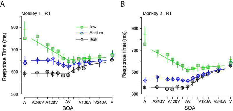
Audiovisual, visual-only and auditory-only mean RTs for both monkeys along with the predicted RT shown in lines according to the diffusion superposition model as a function of SNR (squares = low, diamonds = medium, circles = high) and SOA. Error bars denote confidence intervals (SEM: 2 × standard error of the mean) around predicted mean RTs. Panel A shows the RT for Monkey 1; Panel B shows the RT for Monkey 2. Accuracy is predicted to be at ceiling (see text).

As noted above, the monkeys omitted a substantial proportion of responses to the lowest and medium SNR auditory stimuli and thus had imperfect accuracy. By design, this is not accounted for by the single-barrier Wiener diffusion model. The integral in Equation 3 ranges from 0 to infinity, such that, absorption at the upper barrier is a certain event given enough time. Thus, the Wiener diffusion superposition model always predicts ceiling level accuracies for all intensities, which is obviously inconsistent with the observed behavioral results. A similar argument holds for superposition models based on Ornstein-Uhlenbeck processes (Diederich, 1992, 1995)

Extension 1: The diffusion superposition model with a deadline

An unrealistic assumption of the model described above is that accumulation will always complete, which in the single-barrier Wiener diffusion model implies that the monkeys have 100% detection accuracy (or hit rate). Given enough time, a Wiener diffusion process with drift $\mu >0$ will almost certainly reach the criterion. From an experimental perspective, this has several implications: The intensity of the stimulus components must be sufficiently high to ensure detection rates of 100%, and the temporal window for responding must be infinitely long to guarantee that all responses are collected.

However, if stimulus detection is limited by a deadline $d$ (we assume that the deadline is above the SOA, $d>\tau$) the proportion of correct responses is given by the distribution of the detection times at $t=d$. For unimodal and synchronous audiovisual stimuli, this probability corresponds to the inverse Gaussian distribution at time $d$, $P\left({\mathbf{D}}_i\le d\right)=F_{\text{IG}}\left(d|c,{\mu }_i,{\sigma }_i^2\right)$, with $i$ depending on the modality, $i=\text{A},\text{V},\text{AV}$. The expected detection time, conditional on stimulus detection before $d$, is obtained by integration of $t\cdot f_{\text{IG}}\left(t\right)$ from $t=0$ to $d$ (see Eq. 4), with the solution for the integral given in Schwarz (1994, Eq. 6).

In bimodal stimuli with onset asynchrony $0<\tau <d$ [say, without loss of generality, $\text{V}\left(\tau \right)\text{A}$], it is necessary to distinguish the intervals $\left[0\dots \tau \right]$ and $\left[\tau \dots d\right]$ during which the drift (and the variance) of the diffusion process amount to ${\mu }_{\text{V}}$ (${\sigma }_{\text{V}}^2$) and ${\mu }_{\text{AV}}$ (${\sigma }_{\text{AV}}^2$), respectively. The probability for correct detections amounts to the sum of the detections within $\left[0\dots \tau \right]$ in which only the first stimulus contributes to the buildup of evidence; and the detections within $\left[\tau \dots d\right]$ in which both stimuli are active.

$$\begin{gathered} P\left({\mathbf{D}}_{\text{V}\left(\tau \right)\text{A}}\le d\right)=P\left({\mathbf{D}}_{\text{V}\left(\tau \right)\text{A}}\le \tau \right)+ P\left(\tau <{\mathbf{D}}_{\text{V}\left(\tau \right)\text{A}}\le d\right) \\ =P\left({\mathbf{D}}_{\text{V}}\le \tau \right)+{\int }_{-\infty }^{c}P\left[\mathbf{X}\left(\tau \right)=x\right]\cdot P\left[{\mathbf{D}}_{\text{AV}}\le d-\tau |\mathbf{X}\left(\tau \right)=x\right] dx \\ =F_{\text{IG}}\left(\tau |c,{\mu }_{\text{V}},{\sigma }_{\text{V}}^2\right)+{\int }_{-\infty }^c{w}_{\text{IG}}\left(x,\tau |c,{\mu }_{\text{V}},{\sigma }_{\text{V}}^2\right)\cdot F_{\text{IG}}\left(d-\tau |c-x,{\mu }_{\text{AV}},{\sigma }_{\text{AV}}^2\right) dx \end{gathered}$$ (12)

with $P\left[\mathbf{X}\left(\tau \right)=x\right]=w_{\text{IG}}\left(x,\tau |\cdots \right)$ denoting the density of the activation of the processes not yet absorbed at $t=\tau$ (Eq. 5). The integrand decomposes into a sum of four terms $\varphi \left(x\right)\cdot \text{Φ}\left(x|m,s^2\right)$ that are integrated using a bivariate Normal distribution (Owen, 1980, Eq. 10,010.1, see Appendix A). For the accuracy, an approximate ${\chi }_{26}^2$ statistic is obtained by the squared difference between the predicted and observed proportion of responses, divided by the variance $\pi \left(1-\pi \right)/N$, with $\pi =P\left(\mathbf{D}\le d\right)$ denoting the binomial probabilities for correct detections (e.g., Schwarz, 2006). To avoid numerical problems close to zero or one, $\pi$ was bounded within $\left[0.01, 0.99\right]$.

The expected detection time, conditional on detection before the deadline, amounts to

$$\begin{gathered} E\left({\mathbf{D}}_{\text{V}\left(\tau \right)\text{A}}|{\mathbf{D}}_{\text{V}\left(\tau \right)\text{A}}\le d\hspace{0.17em}\right) \\ \hspace{1em}=\frac{1}{P\left({\mathbf{D}}_{\text{V}\left(\tau \right)\text{A}}\le d\right)}\times [P\left({\mathbf{D}}_{\text{V}\left(\tau \right)\text{A}}\le \tau \right)\cdot E\left({\mathbf{D}}_{\text{V}\left(\tau \right)\text{A}}|{\mathbf{D}}_{\text{V}\left(\tau \right)\text{A}}\le \tau \right)+ P\left(\tau <{\mathbf{D}}_{\text{V}\left(\tau \right)\text{A}}\le d\right)\cdot E\left({\mathbf{D}}_{\text{V}\left(\tau \right)\text{A}}|\tau <{\mathbf{D}}_{\text{V}\left(\tau \right)\text{A}}\le d\right)], \end{gathered}$$ (13)

with $P\left({\mathbf{D}}_{\text{V}\left(\tau \right)\text{A}}\le d\right)$ given by Equation 12. The first term in the brackets is given by Equation 4,

$$\begin{gathered} P\left({\mathbf{D}}_{\text{V}\left(\tau \right)\text{A}}\le \tau \right)\cdot E\left({\mathbf{D}}_{\text{V}\left(\tau \right)\text{A}}|{\mathbf{D}}_{\text{V}\left(\tau \right)\text{A}}\le \tau \right) \\ \hspace{1em}\hspace{1em}=P\left({\mathbf{D}}_{\text{V}}\le \tau \right)\cdot E\left({\mathbf{D}}_{\text{V}}|{\mathbf{D}}_{\text{V}}\le \tau \right) \\ \hspace{1em}\hspace{1em}={\int }_0^{\tau }t\cdot f_{\text{IG}}\left(t|c,{\mu }_{\text{V}},{\sigma }_{\text{V}}^2\right)\hspace{0.17em}dt. \end{gathered}$$ (14)

The second term is more complicated,

$$\begin{gathered} P\left(\tau <{\mathbf{D}}_{\text{V}\left(\tau \right)\text{A}}\le d\right)\cdot E\left({\mathbf{D}}_{\text{V}\left(\tau \right)\text{A}}|\tau <{\mathbf{D}}_{\text{V}\left(\tau \right)\text{A}}\le d\right) \\ \hspace{1em}\hspace{1em}={\int }_{-\infty }^{c}P\left[\mathbf{X}\left(\tau \right)=x\right]\cdot P\left[{\mathbf{D}}_{\text{AV}}\le d-\tau |\mathbf{X}\left(\tau \right)=x\right]\cdot \left\{\tau +E\left[{\mathbf{D}}_{\text{AV}}|\mathbf{X}\left(\tau \right)=x,{\mathbf{D}}_{\text{AV}}\le d-\tau \right]\right\} dx \\ \hspace{1em}\hspace{1em}={\int }_{-\infty }^c{w}_{\text{IG}}\left(x,\tau |c,{\mu }_{\text{V}},{\sigma }_{\text{V}}^2\right)\cdot F_{\text{IG}}\left(d-\tau |c-x,{\mu }_{\text{AV}},{\sigma }_{\text{AV}}^2\right) dx\cdot \tau +{\int }_{-\infty }^c{w}_{\text{IG}}\left(x,\tau |c,{\mu }_{\text{V}},{\sigma }_{\text{V}}^2\right)\cdot {\int }_0^{d-\tau }t\cdot f_{\text{IG}}\left(t|c-x,{\mu }_{\text{AV}},{\sigma }_{\text{AV}}^2\right)\hspace{0.17em}dt dx. \end{gathered}$$ (15)

The $w\cdot G$ term corresponds to Equation 12, multiplied by $\tau$. The double integral decomposes into four ${\int }_{-\infty }^y\varphi \left(x|m_1,s_1^2\right)\cdot \text{Φ}\left(x|m_2,s_2^2\right) dx$ terms (Owen, 1980, Eq. 10,010.1, see Eq. 12 above) and another four terms of the form ${\int }_{-\infty }^{y}x\cdot \varphi \left(x|m_1,s_1^2\right)\cdot \text{Φ}\left(x|m_2,s_2^2\right) dx$ that match with Owen (1980, Eqs: 10,010.1 and 10,011.1).

For the observable mean RT, we assume again an SOA invariant mean residual ${\mu }_{\text{M}}$,

$$E\left(\mathbf{T}\right)=E\left(\mathbf{D}\right)+{\mu }_{\text{M}}$$ (16)

Details are given in Appendix A, with R code (R Core Team, 2017) in the online supplement. For each monkey, an approximate ${\chi }_{25}^2$ goodness-of-fit statistic was determined by the squared standardized deviations of the predicted and the observed average response times. Compared to the model without a deadline, one degree of freedom is lost because the deadline is adjusted to the data. The ${\chi }^2$ for mean RT and accuracy are not independent, however. We therefore did not add them up but instead transformed them into P-values and maximized the minimum of the P-values as a conservative fitting criterion.

Results for the deadline model

Figure 4 shows the results for a Wiener diffusion superposition model with a deadline, fitted to the behavioral performance of the monkeys (accuracy and mean RTs). The deadline parameter improves the model fits and provides a very good description of both accuracy and RTs of the monkeys. For Monkey 1 the model provided an excellent fit to the data (Accuracy: ${\chi }_{26}^2=34.2$; mean RT: ${\chi }_{25}^2=33.0, P_{\text{min}}=0.131$). In Monkey 2, the fit was less convincing (Accuracy: ${\chi }_{26}^2=64.6$; mean RT: ${\chi }_{25}^2=63.1, P_{\text{min}}<0.001$), but acceptable given the conservative fitting procedure where we tried to jointly fit both the RTs and hit rates of the monkeys. Unlike the standard Schwarz (1994) implementation, we found that the Wiener model with a deadline can predict the RT better even for the lowest SNRs.

Figure 4. Wiener diffusion superposition model with a time deadline predicts monkey RTs and response accuracy to audiovisual stimuli. Accuracy and RT of the two monkeys along with the fits from the model.

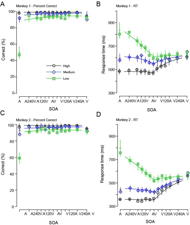
A, C Accuracy of the monkeys as a function of SNR and SOA. X-axes show SOA; Y-axes show the percent correct. B, D Response time of the monkeys as a function of SNR and SOA. X-axes show SOA; Y-axes show mean RT in ms. In both panels, the high SNRS are shown in black circles, the medium SNRs in blue diamonds and low SNRs in green squares. Error bars denote confidence intervals (2 x SEM). The Wiener DSM model with deadline has the ability to fit to both RT and detection accuracy unlike the standard Wiener DSM (cf. Figure 3).

The best fitting parameter estimates are shown in Table 1. Drift rates increased with stimulus intensity (most visible for auditory stimuli), and variances roughly followed this pattern. The deadline was below 1 s, which is consistent with the temporal structure of the task. A substantial residual movement time, ${\mu }_{\text{M}}$, indicates that the model describes about 2/3 of the processing time of a simple response task such as the one used in this study. Taken together, the deadline model provides a good fit to both the accuracy and response time of monkeys performing the detection task. We next compared the fits from the deadline to a two-barrier Wiener diffusion superposition model.

Table 1.

Model parameters for the Wiener superposition model with a deadline

Parameter	Monkey 1	Monkey 2
${\mu }_{\text{A}}$ (low, medium, high)	0.01, 0.25, 1.53	0.09, 0.41, 9.74
${\sigma }_{\text{A}}^2$ (low, medium, high)	18.5, 130.3, 74.4	11.7, 379.6, 10.7
${\mu }_{\text{V}}$ (low, medium, high)	0.35, 0.37, 0.34	0.30, 0.34, 0.37
${\sigma }_{\text{V}}^2$ (low, medium, high)	73.2, 68.0, 92.8	67.8, 73.1, 41.9
${\mu }_{\text{M}}$	419 ms	343 ms
Deadline $d$ (ms)	951 ms	828 ms

Extension 2: Wiener diffusion superposition model with two barriers

In diffusion models for two-choice tasks, evidence accumulation is often described by a Wiener process that evolves between two evidence barriers. As soon as one of these barriers is reached, the respective response is elicited. In the go/no-go task, only one barrier is associated with a response; the other barrier is thought to represent the non-target decision, and the response is withheld. Two-barrier Wiener diffusion models have been quite successful in describing the response times and accuracy rates in choice tasks with two alternatives (Laming, 1968; Luce, 1986; Smith & Ratcliff, 2004; Townsend & Ashby, 1983). Gomez et al. (2007) demonstrated that such a model could successfully describe the response times, false alarms and omission rates in go/no-go tasks with lexical and numerosity decisions. The model was also used to describe the mean RTs and variances in a redundant signals task with go/no-go responses (Blurton et al., 2014).

From a technical perspective, a simple response task with hits, misses, and catch trials like the one used in the present experiment shares similarities with a go/no-go task. We, therefore, evaluated if such a two-barrier diffusion model can account for the observed behavior of the two monkeys. The technical details of such two-barrier models have already been explicated elsewhere (Navarro & Fuss, 2009; Ratcliff et al., 2016; Vandekerckhove & Tuerlinckx, 2008; Wagenmakers, Van Der Maas, & Grasman, 2007). Here, we provide just a summary, focusing on the issues related to the superposition of evidence accumulation in synchronous and asynchronous redundant stimuli.

For single stimuli, evidence accumulation follows a time-homogeneous Wiener process with drift ${\mu }_{\text{A}}>0$, ${\mu }_{\text{V}}>0$ and variance ${\sigma }_{\text{A}}^2>0$, ${\sigma }_{\text{V}}^2>0$. We assume that the process starts at $\mathbf{X}\left(0\right)=0$ and then evolves in time between two constant absorbing barriers $u>0$ and $-\ell <0$. If the upper barrier $u$ is reached first, a response is elicited; if the lower barrier $-\ell$ is reached first, the response is withheld. The barrier-specific first-passage time densities $f_u\left(t\right)$, distributions $F_u\left(t\right)$, mean absorption times $E_u$ and overall absorption probabilities $P_u$ are described in Cox and Miller (1965), Grasman, Wagenmakers, and van der Maas (2009), and Horrocks and Thompson (2004). Efficient numerical implementations for the infinite series for $f_u\left(t\right)$ and distributions $F_u\left(t\right)$ are given by Navarro and Fuss (2009), Blurton, Kesselmeier, and Gondan (2012) and Voss and Voss (2007) for both small and large t (see also Appendix B for further simplifications and optimizations of the calculation).

For synchronously presented redundant stimuli presented, coactivation occurs, resulting in a new Wiener process with drift ${\mu }_{\text{AV}}={\mu }_{\text{A}}+{\mu }_{\text{V}}$ and variance ${\sigma }_{\text{AV}}^2={\sigma }_{\text{A}}^2+{\sigma }_{\text{V}}^2$ (see Eqs. 3 and 4 above). For asynchronous stimuli with onset asynchrony $\tau$ [e.g., $\text{V}\left(\tau \right)\text{A}$], evidence accumulates with drift ${\mu }_{\text{V}}$ and variance ${\sigma }_{\text{V}}^2$ within the first $\tau$ milliseconds. During this interval, an absorption occurs with a probability of $F_u\left(\tau |u, \ell , {\mu }_{\text{V}},{\sigma }_{\text{V}}^2\right)$, given by the “small time series” because $\tau \ll \infty$ (see Gondan, Blurton, & Kesselmeier, 2014, Eq. 3). The expected conditional absorption time $E_u\left(\mathbf{D}|\mathbf{D}\le \tau \right)$ is given by ${\int }_0^{\tau }t\cdot f_u\left(\tau |u, \ell , {\mu }_{\text{V}},{\sigma }_{\text{V}}^2\right)dt$, weighted by $F_u\left(\tau \right)$. Because for small t, the series $f_u$ is an absolutely decreasing, alternating series of weighted inverse Gaussian distributions (see Appendix B), and the second antiderivative of the inverse Gaussian distribution is known (e.g., Schwarz, 1994, Appendix A), the integral can be determined analytically by integrating the components of the series. At time $\tau$, the onset of the second stimulus component, $\mathbf{X}\left(\tau \right)$ ranges somewhere between $-\ell$ and $u$, which is described by the (defective) density $w\left(x, \tau \right)$ (Cox & Miller, 1965, p. 222). As in the single-barrier model (see above Eq. 7), $P_u$ and $E_u$ (both conditional on $\mathbf{D}>\tau$) are then given by the compound of $P_{u-x}$ and $\tau +E_{u-x}$ for drift ${\mu }_{\text{AV}}$ and variance ${\sigma }_{\text{AV}}^2$, weighted by $w\left(x, \tau \right)$, and integrated over all $x\in \left(-\ell ,u\right)$. An analytical solution for ${\int }_{-\ell }^{u}w\left(x,\tau \right)\cdot P_{u-x}\hspace{0.17em}dx$ is given in Appendix B; the integral for $E_u\left(\mathbf{D}|\mathbf{D}>\tau \right)$ must be determined numerically. Absorption probabilities for the lower barrier are obtained by a change of parameters, $\langle u, \ell ,\mu ,{\sigma }^2\rangle \to \langle \ell , u,-\mu ,{\sigma }^2\rangle$.

As before, we allowed one more parameter, ${\mu }_{\text{M}}$, describing the average duration of the residual processes, unrelated to the go/nogo decision. Again, the upper barrier was fixed at $u=100$, and the lower barrier was treated as a free parameter. The pseudo-${\chi }^2$ goodness-of-fit statistic was again given by the worst of ${\chi }^2$ for the mean RTs and the ${\chi }^2$ for the accuracy.

Results for the two-barrier model

Figure 5 shows the results from fitting the diffusion model with two barriers to the behavioral performance of the monkeys (accuracy and mean RTs) as a function of SNR and SOAs (see also Table 2). In both monkeys, the qualitative fits from the two-barrier model to the data were worse than for the deadline model. For instance, both accuracy and response time for the auditory-only SNRs are poorly described, and the model inflates the mean RT for the lowest auditory SNR.

Figure 5. A diffusion superposition model with two barriers is poorer at predicting monkey RTs and response accuracy to audiovisual stimuli.

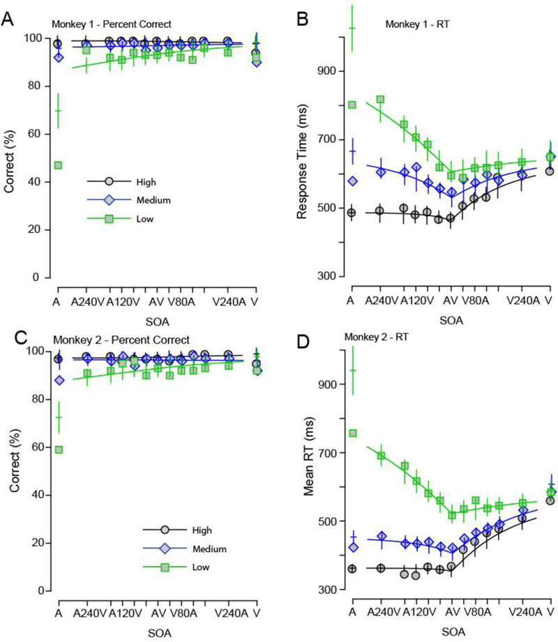
Accuracy and RT of the two monkeys along with the fits from the diffusion superposition model with two barriers. A, C: Accuracy of the monkeys as a function of SNR and SOA. X-axes show SOA; Y-axes show the percent correct. B, D: Response time of the monkeys as a function of SNR and SOA. X-axes show SOA; Y-axes show Response Time in ms. In both panels, the high SNRS are shown in black circles, the medium SNRs in blue diamonds and low SNRs in green squares. Error bars denote confidence intervals (2 x SEM). Note how the two-barrier model fails at predicting the RTs and accuracy for the lowest SNR.

Table 2:

Model parameters for the best fitting two barrier Wiener diffusion superposition model

Parameter	Monkey 1	Monkey 2
${\mu }_{\text{A}}$ (low, medium, high)	0.01, 0.32, 1.13	0.01, 0.59, 1.62
${\sigma }_{\text{A}}^2$ (low, medium, high)	27.2, 45.1, 102.9	30.1, 90.1, 227.6
${\mu }_{\text{V}}$ (low, medium, high)	0.36, 0.37, 0.37	0.32, 0.28 0.35
${\sigma }_{\text{V}}^2$ (low, medium, high)	37.6, 40.8, 43.2	42.0, 45.0, 37.2
$\ell$	205.6	236.0
${\mu }_{\text{M}}$	401 ms	307 ms

These qualitative observations are in close agreement with the quantitative analysis. For both monkeys, the two barrier model provided a rather poor fit to the data (Monkey 1: Accuracy: ${\chi }_{26}^2=105.2$; mean RT: ${\chi }_{25}^2=103.3$, $P_{\text{min}}< 0.001$; Monkey 2: Accuracy: ${\chi }_{26}^2=111.0$; mean RT: ${\chi }_{25}^2=109.1, P_{\text{min}}< 0.001$). These fits were considerably poorer (i.e., larger goodness of fit statistics) than the DSM model with a deadline.

Discussion

The goal of this study was to further describe and understand how the behavioral benefits of multisensory integration during a detection task depended on the intensities of and delays between sensory stimuli. Consistent with many earlier results in bimodal divided attention (Diederich & Colonius, 2004a; Molholm et al., 2002; Murray et al., 2005), separate activation (a.k.a. “race”) models were insufficient to explain the behavioral patterns we observed (Miller, 1982, 1986). We used many SOA conditions, and thus the majority of the stimuli used in the present study were audiovisual in nature. Enrichment of audiovisual conditions rules out effects of trial history and modality shift effects as the exclusive driving force for coactivation effects (Gondan, Lange, Rösler, & Röder, 2004; Miller, 1986; Otto, Dassy, & Mamassian, 2013; Otto & Mamassian, 2012).

The intensity manipulation for the auditory modality was effective (Figure 4). The drift estimates for the deadline model monotonically increased with SNR (Table 1; the variance estimates showed a less regular pattern). In the visual modality, drift and variance estimates were more or less equal for the different intensities, which is consistent with the converging pattern of the mean RTs for positive SOAs (Figure 4). The residual ${\mu }_{\text{M}}$ was similar in the two animals, reflecting their overall response speed and the fact that stimulus detection is probably just out one of several stages of the overall response process.

Our objective was to evaluate simple models that describe how accuracy and response time of observers depend on these factors. We pursued two extensions of the single-barrier Wiener diffusion superposition model (Schwarz, 1989, 1994) to describe both accuracy and RTs of monkeys detecting audiovisual vocalizations of different intensities. A key finding from our study is that incorporating a stopping time for the Wiener diffusion process may help to better model behavior in multisensory detection when multiple SNRs and SOAs are involved. The idea of an internal stopping time or deadline has been put forth by several other authors (Diederich, 2008; Diederich & Oswald, 2016; Ratcliff & Rouder, 2000; Yellott, 1971) and for fixed- and variable-duration tasks (Ratcliff, 2006). These paradigms are often analyzed using deadline models (Busemeyer & Diederich, 2002). In our extension of Schwarz’s (1994) model, we assumed that the observers internally set the deadline (or “optional stopping time”) and therefore we considered it a free parameter and estimated it from the response time data. Addition of this deadline allowed the model to fit both RT and accuracy in the animals.

The deadline model outperformed a two-barrier model with additive superposition of Wiener diffusion processes (Blurton et al., 2014; Gomez et al., 2007). The two-barrier Wiener diffusion models (Ratcliff, 1978; Ratcliff et al., 2016; Smith & Ratcliff, 2004) have been remarkably successful in describing the choice behavior of observers in a large variety of tasks. The primary issue we found with the two-barrier model is that it over-predicted response times for the lower stimulus intensities, a problem recognized previously (Hawkins, Forstmann, Wagenmakers, Ratcliff, & Brown, 2015).

We have limited ourselves to describing and modeling the RT and response accuracy for a detection task across different SNRs and SOAs (Cluff et al., 2015; Crevecoeur et al., 2016; Dixon & Spitz, 1980; Holmes, 2009; Meredith et al., 1987; Stein et al., 1989; van Wassenhove et al., 2007). Some studies have investigated the effect of sensory reliability which shares some similarities to the sensory intensity manipulation we performed here on benefits of multisensory integration but did not modulate the delay between the sensory stimuli (Drugowitsch, DeAngelis, Klier, Angelaki, & Pouget, 2014). Other studies have examined the dependence on sensory delays but not on sensory intensity (Crevecoeur et al., 2016). Experiments that simultaneously vary stimulus intensity, stimulus reliability and SOA may help better understand the relative roles of these factors in multisensory detection and discrimination.

The present study focused on the description of mean RT and accuracy in the single-barrier Wiener diffusion superposition model (Schwarz, 1994). Our unique contribution in this paper was to expand on this model in two ways. We added a single additional parameter (either a deadline or a lower barrier), and to which we were able to provide mathematical or computational improvements (see Appendices A, B, and online supplement). A number of other extensions would be possible, for example, two-barrier models with deadlines and/or collapsing bounds (Diederich & Oswald, 2016; Hawkins et al., 2015). Urgency signals may also provide a better description of the multisensory detection behavior studied here (Ditterich, 2006). Another possible extension is the leaky competing accumulator model (Usher & McClelland, 2001). We anticipate future models will include combinations of these different features to better describe both RT and accuracy in simple and more complex response tasks.

We did not consider diffusion models based on Ornstein-Uhlenbeck processes. In the Ornstein-Uhlenbeck process, the drift is overlaid by a driving force towards a mean reversion level; this model has gained popularity in financial modeling and in neuroscience (Alili, Patie, & Pedersen, 2005; Ricciardi & Sacerdote, 1979; Zhang & Bogacz, 2010). The Ornstein-Uhlenbeck process is a generalization of the Wiener process; if the parameter that controls reversion to the mean set to zero, it specializes to the Wiener process. The process can model leakage or decay in information accumulation, primacy and recency effects in memory, and approach and avoidance effects in decision-making (Busemeyer & Townsend, 1993; Diederich, 1997; Diederich & Busemeyer, 2003). Diederich (1992, 1995) presented a superposition model that assumes additive superposition of Ornstein-Uhlenbeck processes, including an efficient algorithm for approximating the densities and moments of the first passage times in a two-barrier model with absorbing and/or reflecting barriers (Diederich, 1995, 1997; Diederich & Busemeyer, 2003; Smith, 1995, 2000). Similar to the Wiener process with drift, absorption at a single absorbing barrier is a sure event in the Ornstein-Uhlenbeck model (Cox & Miller, 1965); thus, a shift to a more general Ornstein-Uhlenbeck process would not account for reduced accuracy we observed in our experiments. Stated differently, even for the Ornstein-Uhlenbeck process we believe either the extensions proposed here or other extensions described above will be needed to describe the detection accuracy and response times for our data. However, this is needs to be explicitly verified in future work.

We have shown that an accumulator, which integrates visual and auditory inputs to a bound, explained the behavioral benefits from multisensory integration. However, in our task design, no explicit trial onset information was provided to the animals. Instead, the stimulus arrived in a continuous ongoing stream. Our paradigm has several advantages because it mimics a natural flow of stimuli in the real world and avoids sharp transients in visual stimuli. However, it raises the important question of how an integrator knows when to begin integrating the sensory evidence? One plausible solution is that a neural circuit resets the putative integrator after either the last behavioral action by the animal (false alarm/correct detection) or after some time has elapsed (Janssen & Shadlen, 2005). The fits may improve by incorporating previous ideas which propose to jointly model the inter stimulus interval as well as the responses to sensory stimuli.

The model considered here predicts RTs and accuracy of monkeys when they detect dynamic visual and auditory stimuli (vocalizations). In other contexts, generalized variants of these coactivation models have been used with dynamic stimuli (Drugowitsch et al., 2014). The success of the Wiener diffusion superposition model and its generalized versions in explaining behavior for both static and dynamic multisensory stimuli suggests the possibility of common and not different mechanisms for the processing of static and dynamic multisensory stimuli (Raposo, Sheppard, Schrater, & Churchland, 2012). Raposo et al. (2012) showed that rats and humans performing a discrimination task derived behavioral benefits from integrating streams of auditory and visual events. They suggested that the mechanisms used for these pulsatile stimuli are not integrated by typical mechanisms of multisensory integration which they suggested involved close correspondence between auditory and visual inputs to lead to integration—akin to “physiological synchrony” (Meredith et al., 1987). However, the superposition model can process evidence appearing at random times and offset from one another. The superposition model will also show phenomenon such as physiological synchrony—when the intensities are roughly matched maximal benefits occur at or near synchrony (Ulrich & Miller, 1997).

The key contribution was to show that extension of a model with additive superposition of the channel-specific evidence explains the benefits of integrating faces and voices across a wide range of SOAs and SNRs. This class of coactivation models has previously been used to explain response times of human participants in auditory-visual detection tasks (Diederich, 1995; Schwarz, 1989, 1994). The emphasis of these additive coactivation models (or more general versions, e.g., Drugowitsch et al., 2014) is prima facie at odds with classical reports promoting superadditive multisensory interaction (Stein & Meredith, 1993). In these early studies, superadditivity, and other nonlinear mechanisms were considered fundamental for mediating benefits from multisensory integration. However, as a series of more recent studies have shown, the majority of neurons in classical multisensory brain regions often integrate their synaptic input in a linear manner for a range of stimulus intensities. Nonlinearities are observed only at some very low intensities (Dahl, Logothetis, & Kayser, 2010; Populin & Yin, 2002; Skaliora, Doubell, Holmes, Nodal, & King, 2004; Stanford, Quessy, & Stein, 2005; Stanford & Stein, 2007; Stein & Stanford, 2008)—additive combination is the norm. For conflicting stimuli (e.g., in temporal order judgment, where participants are asked to report which modality came first), linear summation may occur in the other direction, with the overall evidence corresponding to the difference between the channel-specific activations (Schwarz, 2006).

Besides linearity of multisensory integration in single neurons, studies increasingly demonstrate that ensembles of neurons (which might encode stimuli nonlinearly at the single neuron level) can perform linear computations (Ma, Beck, Latham, & Pouget, 2006). We believe that the abstract behavioral models presented here might be implemented by adopting frameworks such as probabilistic population codes. Computationally, at the population level, linear summation of neural activation is possible and yields optimal solutions for a very general class of computational problems (Beck et al., 2008; Ma et al., 2006). Extensions of this model showed that assuming Poisson-like distributions of spike counts allows biological networks to accumulate evidence while choosing the most likely action (Beck et al., 2008). We believe our description of behavioral data by a simple formal model will assist in relating neurophysiological and modeling studies of multisensory detection and broadly integration (Chandrasekaran, 2017; Fetsch, DeAngelis, & Angelaki, 2013; Ma et al., 2006; Seilheimer et al., 2014).

Highlights for Chandrasekaran, Blurton, and Gondan, “Audiovisual detection at different intensities and delays”.

• We extend the one-barrier Wiener diffusion superposition model by incorporating a deadline and provide closed-form solutions for detection rate and mean response time for redundant signals tasks with asynchronous stimuli.

• We also provide improved implementations for multisensory detection models based on the two-barrier Wiener diffusion process.

• The deadline model provides the best description of response times and detection rates of two monkeys performing an audiovisual redundant signals task.

Appendix A: Deadline model

A.1. Probability of absorption

Here we derive the explicit expressions for the probability of absorption in bimodal stimuli with onset asynchrony $0<\tau <d$ (Eq. 12) in the Wiener diffusion model with deadline $d$, for the condition $\text{V}\left(\tau \right)\text{A}$. Between $t=0$ and $t=\tau$, only the visual channel contributes to the evidence, so the probability of absorption within the interval $\left(0,\tau \right)$ is given by

$$P\left({\mathbf{D}}_{\text{V}\left(\tau \right)\text{A}}\le \tau \right)=F_{\text{IG}}\left(\tau |c,{\mu }_{\text{V}},{\sigma }_{\text{V}}^2\right)$$ (A.1)

with $F_{\text{IG}}$ denoting the inverse Gaussian distribution (Eq. 2). Later, within $\left(\tau ,d\right)$, the probability of absorption is a mixture of absorption probabilities of the processes still active at time $\tau$, with the barrier depending on the activation $\mathbf{X}\left(\tau \right)<c$, weighted by their density:

$$P\left(\tau <{\mathbf{D}}_{\text{V}\left(\tau \right)\text{A}}\le d\right)={\int }_{-\infty }^c{w}_{\text{IG}}\left(x,\tau |c,{\mu }_{\text{V}},{\sigma }_{\text{V}}^2\right)\cdot F_{\text{IG}}\left(d^{\prime }|c-x,{\mu }_{\text{AV}},{\sigma }_{\text{AV}}^2\right) dx,$$ (A.2)

with $d^{\prime }=d-\tau$, and $w_{\text{IG}}$ given by Equation 5. The integrand in (A.2) can be transformed into four integrals of the form $q{\int }_{-\infty }^c\text{exp}\left(rx\right)\varphi \left(x|m_1,s_1^2\right)\cdot \text{Φ}\left(x|m_2,s_2^2\right)\hspace{0.17em}dx$:

$$\begin{gathered} {\int }_{-\infty }^c{w}_{\text{IG}}\left(x,\tau |c,{\mu }_{\text{V}},{\sigma }_{\text{V}}^2\right)\cdot F_{\text{IG}}\left(d^{\prime }|c-x,{\mu }_{\text{AV}},{\sigma }_{\text{AV}}^2\right) dx \\ ={\int }_{-\infty }^c\varphi \left(x|{\mu }_{\text{V}}\tau ,{\sigma }_{\text{V}}^2\tau \right)\text{ Φ}\left(x|c-{\mu }_{\text{AV}}{d}^{\prime },{\sigma }_{\text{AV}}^2{d}^{\prime }\right) dx \\ \hspace{1em}+\text{exp}\left(\frac{2c{\mu }_{\text{AV}}}{{\sigma }_{\text{AV}}^2}\right){\int }_{-\infty }^c\text{exp}\left(-\frac{2{\mu }_{\text{AV}}}{{\sigma }_{\text{AV}}^2}x\right)\hspace{0.17em}\varphi \left(x|{\mu }_{\text{V}}\tau ,{\sigma }_{\text{V}}^2\tau \right)\text{Φ}\left(x|c+{\mu }_{\text{AV}}{d}^{\prime },{\sigma }_{\text{AV}}^2{d}^{\prime }\right) dx \\ \hspace{1em}-\text{exp}\left(\frac{2c{\mu }_{\text{V}}}{{\sigma }_{\text{V}}^2}\right){\int }_{-\infty }^c\varphi \left(x|2c+{\mu }_{\text{V}}\tau ,{\sigma }_{\text{V}}^2\tau \right)\text{ Φ}\left(x|c-{\mu }_{\text{AV}}{d}^{\prime },{\sigma }_{\text{AV}}^2{d}^{\prime }\right) dx \\ \hspace{1em}-\text{exp}\left(\frac{2c{\mu }_{\text{V}}}{{\sigma }_{\text{V}}^2}+\frac{2c{\mu }_{\text{AV}}}{{\sigma }_{\text{AV}}^2}\right){\int }_{-\infty }^c\text{exp}\left(-\frac{2{\mu }_{\text{AV}}}{{\sigma }_{\text{AV}}^2}x\right)\hspace{0.17em}\varphi \left(x|2c+{\mu }_{\text{V}}\tau ,{\sigma }_{\text{V}}^2\tau \right)\text{ Φ}\left(x|c+{\mu }_{\text{AV}}{d}^{\prime },{\sigma }_{\text{AV}}^2{d}^{\prime }\right) dx \end{gathered}$$

By completing the square, we have $\text{exp}\left(rx\right)\varphi \left(x|m_1,s_1^2\right)=\text{exp}\left(r{m}_1+r^2{s}_1^2/2\right)\varphi \left(x|m_1^{\text{'}},s_1^2\right)$, with $m_1^{\text{'}}=m_1+r{s}_1^2$. This yields

$$\begin{gathered} {\int }_{-\infty }^c\varphi \left(x|m_1^{\text{'}},s_1^2\right)\cdot \text{Φ}\left(x|m_2,s_2^2\right) dx={\int }_{-\infty }^{\left(c-m_1^{\prime }\right)/s_1}\varphi \left(z\right)\cdot \text{Φ}\left(z|\frac{m_2-m_1^{\prime }}{s_1},\frac{s_2^2}{s_1^2}\right) dz \\ ={\int }_{-\infty }^{\left(c-m_1^{\prime }\right)/s_1}\varphi \left(z\right)\cdot \text{Φ}\left(\frac{s_1}{s_2}z+\frac{m_1^{\prime }-m_2}{s_2}\right) du, \end{gathered}$$ (A.3)

Let $z=\frac{x-m_1^{\text{'}}}{s_1}$, or $x=z{s}_1+m_1^{\text{'}}$. The result in A.3 matches Eq. 10,010.1 in Owen (1980) and is determined by the bivariate Normal distribution, ${\int }_{-\infty }^y\varphi \left(u\right)\cdot \text{Φ}\left(a+bu\right)du=\text{ΦΦ}\left(\frac{a}{\sqrt{1+b^2}},y|\varrho =-\frac{b}{\sqrt{1+b^2}}\right)$.

A.2. Conditional mean response time

We now derive analytic expressions for the mean response time, conditional on absorption before the deadline (Eqs. 13–15 in the main text). Without loss of generality, we consider again the case $\text{V}\left(\tau \right)\text{A}$. Between $t=0$ and $t=\tau$, only one channel contributes to the evidence, so the mean RT is given by Schwarz (1994, Equation A.2):

$$\begin{gathered} P\left({\mathbf{D}}_{\text{V}\left(\tau \right)\text{A}}\le \tau \right)\cdot E\left({\mathbf{D}}_{\text{V}\left(\tau \right)\text{A}}|{\mathbf{D}}_{\text{V}\left(\tau \right)\text{A}}\le \tau \right) \\ \hspace{1em}={\int }_0^{\tau }t f_{\text{IG}}\left(t|c,{\mu }_{\text{V}},{\sigma }_{\text{V}}^2\right)\hspace{0.17em}dt \\ \hspace{1em}=\frac{c}{{\mu }_{\text{V}}}\left[\text{Φ}\left({\mu }_{\text{V}}\tau |c,{\sigma }_{\text{V}}^2\tau \right)-\text{exp}\left(\frac{2c{\mu }_{\text{V}}}{{\sigma }_{\text{V}}^2}\right)\text{Φ}\left(-{\mu }_{\text{V}}\tau |c,{\sigma }_{\text{V}}^2\tau \right)\right] \end{gathered}$$ (A.4)

Within $\left(\tau ,d\right)$, the expected detection time is again a compound of expectations of the processes still active at time $\tau$, weighted by the density of $\mathbf{X}\left(\tau \right)$. The drift and the variance (${\mu }_{\text{AV}}$, ${\sigma }_{\text{AV}}^2$) are increased, because both stimuli are shown, and the work to be done (i.e., the distance between the barrier and the state of the process at time $\tau$) depends on $\mathbf{X}\left(\tau \right)<c$. Because since stimulus onset, $\tau$ ms have already passed, the time scale is shifted, $d^{\prime }=d-\tau$.

$$\begin{gathered} P\left(\tau <{\mathbf{D}}_{\text{V}\left(\tau \right)\text{A}}\le d\right)\cdot E\left({\mathbf{D}}_{\text{V}\left(\tau \right)\text{A}}|\tau <{\mathbf{D}}_{\text{V}\left(\tau \right)\text{A}}\le d\right) \\ \hspace{1em}={\int }_{-\infty }^{c}P\left[\mathbf{X}\left(\tau \right)=x\right]\cdot P\left({\mathbf{D}}_{\text{AV}}\le d^{\prime }|\mathbf{X}\left(\tau \right)=x\right)\cdot \left\{\tau +E\left[{\mathbf{D}}_{\text{AV}}|\mathbf{X}\left(\tau \right)=x,{\mathbf{D}}_{\text{AV}}\le d^{\prime }\right] dx\right\} \\ \hspace{1em}={\int }_{-\infty }^c{w}_{\text{IG}}\left(x,\tau |c,{\mu }_{\text{V}},{\sigma }_{\text{V}}^2\right)\cdot F_{\text{IG}}\left(d^{\prime }|c-x,{\mu }_{\text{AV}},{\sigma }_{\text{AV}}^2\right) dx\cdot \tau \\ \hspace{1em}\hspace{1em}+{\int }_{-\infty }^c{w}_{\text{IG}}\left(x,\tau |c,{\mu }_{\text{V}},{\sigma }_{\text{V}}^2\right)\cdot {\int }_0^{d^{\prime }}t\cdot f_{\text{IG}}\left(t|c-x,{\mu }_{\text{AV}},{\sigma }_{\text{AV}}^2\right)dt dx \end{gathered}$$ (A.5)

The first term corresponds exactly to (A.2), multiplied by the onset asynchrony $\tau$. For the bounded integral ${\int }_0^{d^{\prime }}t\cdot f_{\text{IG}}\left(t \text{|} c-x,{\mu }_{\text{AV}},{\sigma }_{\text{AV}}^2\right) dt$, the solution is again found in the appendix in Schwarz (1994, Equation A.2).

The double integral in (A.5) is

$$\begin{gathered} {\int }_{-\infty }^c\left[\varphi \left(x|{\mu }_{\text{V}}\tau ,{\sigma }_{\text{V}}^2\tau \right)-\text{exp}\left(\frac{2c{\mu }_{\text{V}}}{{\sigma }_{\text{V}}^2}\right)\cdot \varphi \left(x|2c+{\mu }_{\text{V}}\tau ,{\sigma }_{\text{V}}^2\tau \right)\right] \\ \hspace{1em}\times \frac{c-x}{{\mu }_{\text{AV}}}\cdot \left[\text{Φ}\left(x|c-{\mu }_{\text{AV}}{d}^{\prime },{\sigma }_{\text{AV}}^2{d}^{\prime }\right)-\text{exp}\left(\frac{2\left(c-x\right){\mu }_{\text{AV}}}{{\sigma }_{\text{AV}}^2}\right)\text{Φ}\left(x|c+{\mu }_{\text{AV}}{d}^{\prime },{\sigma }_{\text{AV}}^2{d}^{\prime }\right)\right] dx \\ =\frac{c}{{\mu }_{\text{AV}}}{\int }_{-\infty }^c\varphi \left(x|{\mu }_{\text{V}}\tau ,{\sigma }_{\text{V}}^2\tau \right)\text{ Φ}\left(x|c-{\mu }_{\text{AV}}{d}^{\prime },{\sigma }_{\text{AV}}^2{d}^{\prime }\right) dx \\ \hspace{1em}-\frac{c}{{\mu }_{\text{AV}}}\text{exp}\left(\frac{2c{\mu }_{\text{V}}}{{\sigma }_{\text{V}}^2}\right){\int }_{-\infty }^c\varphi \left(x|2c+{\mu }_{\text{V}}\tau ,{\sigma }_{\text{V}}^2\tau \right)\text{ Φ}\left(x|c-{\mu }_{\text{AV}}{d}^{\prime },{\sigma }_{\text{AV}}^2{d}^{\prime }\right) dx \\ \hspace{1em}-\frac{c}{{\mu }_{\text{AV}}}\text{exp}\left(\frac{2c{\mu }_{\text{AV}}}{{\sigma }_{\text{AV}}^2}\right){\int }_{-\infty }^c\text{exp}\left(-\frac{2{\mu }_{\text{AV}}x}{{\sigma }_{\text{AV}}^2}\right)\hspace{0.17em}\varphi \left(x|{\mu }_{\text{V}}\tau ,{\sigma }_{\text{V}}^2\tau \right)\text{ Φ}\left(x|c+{\mu }_{\text{AV}}{d}^{\prime },{\sigma }_{\text{AV}}^2{d}^{\prime }\right) dx \\ \hspace{1em}+\frac{c}{{\mu }_{\text{AV}}}\text{exp}\left(\frac{2c{\mu }_{\text{V}}}{{\sigma }_{\text{V}}^2}+\frac{2c{\mu }_{\text{AV}}}{{\sigma }_{\text{AV}}^2}\right){\int }_{-\infty }^c\text{exp}\left(\frac{-2{\mu }_{\text{AV}}x}{{\sigma }_{\text{AV}}^2}\right)\hspace{0.17em}\varphi \left(x|2c+{\mu }_{\text{V}}\tau ,{\sigma }_{\text{V}}^2\tau \right)\text{Φ}\left(x|c+{\mu }_{\text{AV}}{d}^{\prime },{\sigma }_{\text{AV}}^2{d}^{\prime }\right) dx \\ \hspace{1em}-\frac{1}{{\mu }_{\text{AV}}}{\int }_{-\infty }^{c}x \varphi \left(x|{\mu }_{\text{V}}\tau ,{\sigma }_{\text{V}}^2\tau \right)\text{ Φ}\left(x|c-{\mu }_{\text{AV}}{d}^{\prime },{\sigma }_{\text{AV}}^2{d}^{\prime }\right) dx \\ \hspace{1em}+\frac{1}{{\mu }_{\text{AV}}}\text{exp}\left(\frac{2c{\mu }_{\text{V}}}{{\sigma }_{\text{V}}^2}\right){\int }_{-\infty }^{c}x \varphi \left(x|2c+{\mu }_{\text{V}}\tau ,{\sigma }_{\text{V}}^2\tau \right)\text{ Φ}\left(x|c-{\mu }_{\text{AV}}{d}^{\prime },{\sigma }_{\text{AV}}^2{d}^{\prime }\right) dx \\ \hspace{1em}+\frac{1}{{\mu }_{\text{AV}}}\text{exp}\left(\frac{2c{\mu }_{\text{AV}}}{{\sigma }_{\text{AV}}^2}\right){\int }_{-\infty }^{c}x \text{exp}\left(-\frac{2{\mu }_{\text{AV}}x}{{\sigma }_{\text{AV}}^2}\right)\varphi \left(x|{\mu }_{\text{V}}\tau ,{\sigma }_{\text{V}}^2\tau \right)\text{ Φ}\left(x|c+{\mu }_{\text{AV}}{d}^{\prime },{\sigma }_{\text{AV}}^2{d}^{\prime }\right) dx \\ \hspace{1em}-\frac{1}{{\mu }_{\text{AV}}}\text{exp}\left(\frac{2c{\mu }_{\text{V}}}{{\sigma }_{\text{V}}^2}+\frac{2c{\mu }_{\text{AV}}}{{\sigma }_{\text{AV}}^2}\right){\int }_{-\infty }^{c}x \text{exp}\left(-\frac{2{\mu }_{\text{AV}}x}{{\sigma }_{\text{AV}}^2}\right)\varphi \left(x\text{|}2c+{\mu }_{\text{V}}\tau ,{\sigma }_{\text{V}}^2\tau \right)\text{Φ}\left(x\text{|}c+{\mu }_{\text{AV}}{d}^{\prime },{\sigma }_{\text{AV}}^2{d}^{\prime }\right) dx \end{gathered}$$ (A.6)

The first four terms correspond to (A.3). By completing the square, we have $\text{exp}\left(rx\right)\varphi \left(x|m_1,s_1^2\right)=\text{exp}\left(r{m}_1+r^2{s}_1^2/2\right)\varphi \left(x|m_1^{\text{'}},s_1^2\right)$, with $m_1^{\text{'}}=m_1+r{s}_1^2$. Let $u=\frac{x-m_1^{\text{'}}}{s_1}$, or $x=m_1^{\text{'}}+u{s}_1$. Then,

$$\begin{gathered} {\int }_{-\infty }^{c}x\cdot \varphi \left(x|m_1^{\prime },s_1^2\right)\cdot \text{Φ}\left(x|m_2,s_2^2\right) dx \\ \hspace{1em}={\int }_{-\infty }^{\left(c-m_1^{\prime }\right)/s_1}\left(m_1^{\prime }+u{s}_1\right)\cdot \varphi \left(u|0, 1\right)\cdot \text{Φ}\left(u|\frac{m_2-m_1^{\prime }}{s_1},\frac{s_2^2}{s_1^2}\right) du \\ \hspace{1em}=m_1^{\prime }\cdot {\int }_{-\infty }^{\left(c-m_1^{\prime }\right)/s_1}\varphi \left(u|0, 1\right)\cdot \text{Φ}\left(\frac{s_1}{s_2}u+\frac{m_1^{\prime }-m_2}{s_2}|0, 1\right) du \\ \hspace{1em}\hspace{1em}+s_1\cdot {\int }_{-\infty }^{\left(c-m_1^{\prime }\right)/s_1}u\cdot \varphi \left(u|0, 1\right)\cdot \text{Φ}\left(\frac{s_1}{s_2}u+\frac{m_1^{\prime }-m_2}{s_2}|0, 1\right) du \end{gathered}$$ (A.7)

The first term of (A.7) matches Eq. 10,010.1 in Owen (1980). The second term matches Eq. 10,011.1, ${\int }_{-\infty }^{y}u\cdot \varphi \left(u\right)\cdot \text{Φ}\left(a+bu\right) du=\frac{b}{\sqrt{1+b^2}}\cdot \varphi \left(\frac{b}{\sqrt{1+b^2}}\right)\cdot \text{Φ}\left(y\sqrt{1+b^2}+\frac{ab}{\sqrt{1+b^2}}\right)-\varphi \left(y\right)\cdot \text{Φ}\left(a+bu\right)$.

Appendix B: Two-Barrier Wiener diffusion model with two stages

In this appendix we provide solutions for detection accuracy and first-passage times in Wiener diffusion model (Navarro & Fuss, 2009; Ratcliff et al., 2016; Vandekerckhove & Tuerlinckx, 2008; Wagenmakers et al., 2007) with two processing stages. In the single-stage model, evidence accumulation is described by a time-homogeneous Wiener process with drift $\mu$ and variance ${\sigma }^2>0$, starting at $\mathbf{X}\left(0\right)=0$ and then randomly moving between two constant absorbing barriers $u>0$ and $-\ell <0$. Two representations exist, both infinite series (Cox & Miller, 1965), for the first-passage time densities $f_u\left(t\right)$ and their distribution $F_u\left(t\right)$ at the upper barrier; the respective expressions for the lower barrier are obtained by a change of parameters, $\langle u, \ell ,\mu ,{\sigma }^2\rangle \to \langle \ell , u,-\mu ,{\sigma }^2\rangle$. One representation (Feller, 1968, Ch. 14, Eq. 6.15) converges best for large t, the other representation (Feller, 1968, Ch. 14, Problem 22) converges best for small t (Navarro & Fuss, 2009). For the purpose of the present study, $f_u\left(\tau \right)$, $F_u\left(\tau \right)$, and ${\int }_0^{\tau }t\cdot f_u\left(t\right) dt$ need to be determined for small times (i.e., the SOA, $\tau$), so we will first focus on the small-time representation. The series typically refers to the “sub-survivor” function (e.g., Ratcliff, 1978, A8 and A12), but can be restated as a weighted infinite sum of inverse Gaussian distributions,

$$\begin{gathered} F_u\left(t|u, -\ell ,\mu ,{\sigma }^2\right) \\ \hspace{1em}={\sum }_{k=0}^{\infty }\text{exp}\left(-\frac{r_{2k}\mu }{{\sigma }^2}\right)F_{\text{IG}}\left(t|r_{2k}+u,\mu ,{\sigma }^2\right)-\text{exp}\left(\frac{-r_{2k+1}\mu +2u\mu }{{\sigma }^2}\right)F_{\text{IG}}\left(t|r_{2k+1}-u,\mu ,{\sigma }^2\right), \end{gathered}$$ (B.1)

with $r_j=j\left(u+\ell \right)$, and $F_{\text{IG}}\left(t|c,\mu ,{\sigma }^2\right)$ denoting the inverse Gaussian distribution function (e.g., Folks & Chhikara, 1978, Eq. 7). Expression B.1 is an alternating, absolutely decreasing series (Gondan et al., 2014), so it can be truncated at a fixed tolerance $\epsilon >0$ whenever an individual term is below $\epsilon$. The density $f_u\left(\tau \right)$ is, thus, easily obtained by the derivative of the individual terms,

$$\begin{gathered} f_u\left(t|u, -\ell ,\mu ,{\sigma }^2\right) \\ \hspace{1em}={\sum }_{k=0}^{\infty }\text{exp}\left(-\frac{r_{2k}\mu }{{\sigma }^2}\right)f_{\text{IG}}\left(t|r_{2k}+u,\mu ,{\sigma }^2\right)-\text{exp}\left(\frac{-r_{2k+1}\mu +2u\mu }{{\sigma }^2}\right)f_{\text{IG}}\left(t|r_{2k+1}-u,\mu ,{\sigma }^2\right) \end{gathered}$$ (B.2)

At time $\tau$, the density of the processes that have not yet been absorbed is described by the following series (Cox & Miller, 1965, Eq. 78),

$$\begin{gathered} w_{2\text{B}}\left(x,\tau |u,-\ell ,\mu ,{\sigma }^2\right) \\ \hspace{1em}={\sum }_{k=-\infty }^{\infty }\left[\text{exp}\left(\frac{\mu r_{2k}}{{\sigma }^2}\right)\varphi \left(x|r_{2k}+\mu \tau ,{\sigma }^2\tau \right)-\text{exp}\left(\frac{\mu r_{2k}^{\prime }}{{\sigma }^2}\right)\varphi \left(x|r_{2k}^{\prime }+\mu \tau ,{\sigma }^2\tau \right)\right], \end{gathered}$$ (B.3a)

with again $r_j=j\left(u+\ell \right)$ and $r_j^{\text{'}}=2u-r_j$, and good convergence for large drift. The alternative representation (Cox & Miller, 1965, Eq. 81) shows good convergence for small drift,

$$\begin{gathered} w_{2\text{B}}\left(x,\tau |u,-\ell ,\mu ,{\sigma }^2\right) \\ \hspace{1em}=\text{exp}\left(\frac{\mu }{{\sigma }^2}x\right){\sum }_{k=1}^{\infty }{a}_k\cdot \text{exp}\left(-{\lambda }_{k}t\right)\text{sin}\left[b_k\left(x+\ell \right)\right], \end{gathered}$$ (B.3b)

with $a_k=\frac{2}{u+\ell }\cdot \text{sin}\left(\frac{k\pi \ell }{u+\ell }\right), b_k\text{:=}\frac{k\pi }{u+\ell },{\lambda }_k=\frac{1}{2}\left(\frac{{\mu }^2}{{\sigma }^2}+b_k^2{\sigma }^2\right)$. Cox and Miller characterize both series as absolutely convergent. The antiderivative for the large-drift series is obtained by term-wise integration, it converges for positive drift (the value for negative drift is obtained by shift of parameters);

$$\begin{gathered} W_{2\text{B}}\left(x,\tau |u,-\ell ,\mu ,{\sigma }^2\right)= \\ \hspace{1em}f\left(x\right)=\{\begin{array}{c}{\sum }_{k=-\infty }^{\infty }\left[\text{exp}\left(\frac{\mu r_{2k}}{{\sigma }^2}\right)\text{Φ}\left(x|r_{2k}+\mu \tau ,{\sigma }^2\tau \right)-\text{exp}\left(\frac{\mu r_{2k}^{\prime }}{{\sigma }^2}\right)\text{Φ}\left(x|r_{2k}^{\prime }+\mu \tau ,{\sigma }^2\tau \right)\right], \text{for} \mu \gg 0\\ -W_{2\text{B}}\left(-x,\tau |\ell ,-u,-\mu ,{\sigma }^2\right), \text{for} \mu \ll 0\end{array} \end{gathered}$$ (B.4a)

The series can be reordered and decomposed into two branches,

$${\sum }_{k=-\infty }^{\infty }\left[s\left(k\right)-s^{\prime }\left(k\right)\right]={\sum }_{k=0}^{\infty }\left[s\left(k\right)-s^{\prime }\left(-k\right)\right]-{\sum }_{k=1}^{\infty }\left[s^{\prime }\left(k\right)-s\left(-k\right)\right],$$

with $s\left(k\right)=$ $\text{exp}\left(\frac{\mu r_{2k}}{{\sigma }^2}\right)\cdot \text{Φ}\left(x|r_{2k}+\mu \tau ,{\sigma }^2\tau \right)$ and $s^{\prime }\left(k\right)=$ $\text{exp}\left(\frac{\mu r_{-2k}^{\prime }}{{\sigma }^2}\right)\cdot \text{Φ}\left(x|r_{-2k}^{\prime }+\mu \tau ,{\sigma }^2\tau \right)$. The sub-series are both absolutely decreasing, alternating series, that is, $s\left(k\right)>s^{\prime }\left(-k\right)>s\left(k+1\right)>s^{\prime }\left(-\left(k+1\right)\right)>\cdots$, and $s^{\prime }\left(k\right)>s\left(-k\right)>s^{\prime }\left(k+1\right)>s\left(-\left(k+1\right)\right)>\cdots$, so that evaluation of the series can stop as soon as the size of an individual term is below a specific truncation tolerance $\epsilon$.

We illustrate it for $s\left(k\right)>s^{\prime }\left(-k\right)$; the proofs for other the inequalities are very similar. Simplifications arithmetic transformations lead to a ratio of Normal integrals

$$\frac{\text{Φ}\left(x|r_{2k}+\mu \tau ,{\sigma }^2\tau \right)}{\text{Φ}\left(x|2u+r_{2k}+\mu \tau ,{\sigma }^2\tau \right)}>\text{exp}\left(\frac{2\mu u}{{\sigma }^2}\right),$$

which is above the criterion if the same criterion holds for the respective densities,

$$\frac{\varphi \left(x|r_{2k}+\mu \tau ,{\sigma }^2\tau \right)}{\varphi \left(x|2u+r_{2k}+\mu \tau ,{\sigma }^2\tau \right)}>\text{exp}\left(\frac{2\mu u}{{\sigma }^2}\right).$$

After taking the logarithm, simplifying and cancellation of double terms, the inequality reduces to $r_{2k}>x-u$, which is fulfilled for all k (in the branches, $k>0$) because $-\ell <x<u$ by definition.

For small drift, integration of Expression B.3b yields

$$\begin{gathered} W_{2\text{B}}\left(x,\tau |u,-\ell ,\mu ,{\sigma }^2\right)= \\ \hspace{1em}\hspace{1em}{\sigma }^2\cdot \text{exp}\left(\frac{\mu x}{{\sigma }^2}\right)\cdot {\sum }_{k=1}^{\infty }\frac{a_k\cdot \text{exp}\left(-{\lambda }_k\tau \right)}{{\mu }^2+b_k^2{\sigma }^4}\cdot \left\{\mu \hspace{0.17em}\text{sin}\left[b_k\left(x+\ell \right)\right]-b_k{\sigma }^2\cdot \text{cos}\left[b_k\left(x+\ell \right)\right]\right\} \end{gathered}$$ (B.4b)

In order to decide which representation is used (e.g., for drifts close to zero), the number $K$ of required terms of the series can be estimated in advance for a desired truncation error $\epsilon >0$ (Navarro & Fuss, 2009), and then the series with least computational cost can be chosen. For the large-drift representation (B.4a), which is absolutely decreasing and alternating, we need $K$ terms such that $s_k,s_{-k},s_k^{\text{'}},s_{-k}^{\text{'}}<\epsilon$; this is established if $\text{exp}\left(-\frac{\mu r_{2K}}{{\sigma }^2}\right)<\epsilon$, or $K>-\frac{{\sigma }^2\cdot \log \epsilon }{\left(u+\ell \right)\mu }$. For the small-drift expression (B.4b), $K$ needs to fulfil $\text{Φ}\left(K|0,\frac{{\left(u+\ell \right)}^2}{{\pi }^2{\sigma }^2\tau }\right)\ge 1-{\epsilon }^{\prime }$, with ${\epsilon }^{\prime }=\epsilon \cdot \frac{\pi {\sigma }^2}{2}\cdot \sqrt{\frac{\pi {\sigma }^2\tau }{2{\left(u+\ell \right)}^2}}\cdot \text{exp}\left(-\frac{\mu x}{{\sigma }^2}+\frac{{\mu }^2\tau }{2{\sigma }^2}\right)/\left(\frac{\left(u+\ell \right)\mu }{\pi }+{\sigma }^2\right)$.

B.1. Probability of absorption

We now consider the overall absorption probability at the upper barrier. In the single-stage process (i.e., for single and synchronous redundant stimuli), the probability is given by

$$P_u=F_u\left(\infty |u,-\ell ,\mu ,{\sigma }^2\right)={\int }_0^{\infty }{f}_u\left(t\right) dt=\frac{\text{exp}\left(-2\ell \mu /{\sigma }^2\right)-1}{\text{exp}\left[-2\left(u+\ell \right)\mu /{\sigma }^2\right]-1}$$ (B.5)

(e.g., Horrocks & Thompson, 2004). In the two-stage process (e.g., $\text{V}\left(\tau \right)\text{A}$), upper absorptions occur either before $\tau$, with probability $F_u\left(\tau |u,-\ell ,{\mu }_{\text{V}},{\sigma }_{\text{V}}^2\right)$. Alternatively, absorption occurs after $\tau$, with the probability given by the integrated weighted compound of the not-yet-absorbed processes at that time,

$${\int }_{-\ell }^u{w}_{2\text{B}}\left(x,\tau |u,-\ell ,{\mu }_{\text{V}},{\sigma }_{\text{V}}^2\right)\cdot F_u\left[\infty |u-x,-\left(\ell +x\right),{\mu }_{\text{AV}},{\sigma }_{\text{AV}}^2\right] dx$$ (B.6)

with $F_u\left(\infty \right)$ given by (B.5), for the new barriers $u-x$ and $-\left(\ell +x\right)$, and $w_{2\text{B}}$ denoting the density of the not-yet-absorbed processes in the two-barrier situation (see above Eqs. B.3a and B.3b). In Expression B.6, the upper and lower barriers in $P_u$ (B.4) are replaced by $u-x$ and $-\left(\ell +x\right)$, respectively, such that only the numerator depends on $x$.

The integral in (B.6) is then easily obtained. Let ${\mu }^{\prime }=\frac{{\mu }_{\text{V}}}{{\sigma }_{\text{V}}^2}-\frac{2{\mu }_{\text{AV}}}{{\sigma }_{\text{AV}}^2}$. Then, for ${\mu }^{\prime }\gg 0$, we have,

$$\begin{gathered} \int w_{2\text{B}}\left(x,\tau |u,-\ell ,{\mu }_{\text{V}},{\sigma }_{\text{V}}^2\right)\cdot F_u\left[\infty |u-x,-\left(\ell +x\right),{\mu }_{\text{AV}},{\sigma }_{\text{AV}}^2\right] dx \\ \hspace{1em}=\frac{1}{1-\text{exp}\left[-\frac{2\left(u+\ell \right){\mu }_{\text{AV}}}{{\sigma }_{\text{AV}}^2}\right]}\times \{W_{2\text{B}}\left(x,\tau |u,-\ell ,{\mu }_{\text{V}},{\sigma }_{\text{V}}^2\right)-\left[2{\sigma }_{\text{V}}^2\tau {\left(\frac{{\mu }_{\text{AV}}}{{\sigma }_{\text{AV}}^2}\right)}^2-2\left(\ell +{\mu }_{\text{V}}\tau \right)\frac{{\mu }_{\text{AV}}}{{\sigma }_{\text{AV}}^2}\right]\cdot \\ \hspace{1em}{\sum }_{k=-\infty }^{\infty }\left[\text{exp}\left({\mu }^{\prime }{r}_{2k}\right)\text{Φ}\left(x|r_{2k}+\mu \prime {\sigma }_{\text{V}}^2\tau ,{\sigma }_{\text{V}}^2\tau \right)-\text{exp}\left({\mu }^{\prime }{r}_{2k}^{\prime }\right)\text{Φ}\left(x|r_{2k}^{\prime }+\mu \prime {\sigma }_{\text{V}}^2\tau ,{\sigma }_{\text{V}}^2\tau \right)\right]\}, \end{gathered}$$ (B.7a)

which is an alternating and absolutely decreasing series and converges when $\text{exp}\left({\mu }^{\prime }{r}_{-2k}\right)\le \epsilon$ (see B.3a). For ${\mu }^{\prime }\ll 0$, we evaluate $-{\int }_{-u}^{\ell }{w}_{2\text{B}}\left(x,\tau |\ell ,-u,-{\mu }_{\text{V}},{\sigma }_{\text{V}}^2\right)\cdot F_u\left[\infty |\ell -x,-\left(u+x\right),-{\mu }_{\text{AV}},{\sigma }_{\text{AV}}^2\right] dx$. For ${\mu }^{\prime }\approx 0$, we integrate the “small-drift” representation (Cox & Miller, 1965, Eq. 81) to obtain the antiderivative

$$\begin{gathered} \int w_{2\text{B}}\left(x,\tau |u,-\ell ,{\mu }_{\text{V}},{\sigma }_{\text{V}}^2\right)\cdot F_u\left[\infty |u-x,-\left(\ell +x\right),{\mu }_{\text{AV}},{\sigma }_{\text{AV}}^2\right] dx \\ \hspace{1em}=\frac{1}{1-\text{exp}\left[-\frac{2\left(u+\ell \right){\mu }_{\text{AV}}}{{\sigma }_{\text{AV}}^2}\right]}\times \{W_{2\text{B}}\left(x,\tau |u,-\ell ,{\mu }_{\text{V}},{\sigma }_{\text{V}}^2\right) \\ \hspace{1em}\hspace{1em}-\text{exp}\left(-\frac{2\ell {\mu }_{\text{AV}}}{{\sigma }_{\text{AV}}^2}\right){\sum }_{k=1}^{\infty }\frac{a_k\cdot \exp \left({\mu }^{\prime }x-{\lambda }_{k}t\right)}{b_k^2+{{\mu }^{\prime }}^2}\cdot \left({\mu }^{\prime }\text{sin}\left[b_k\left(x+\ell \right)\right]-b_k\text{cos}\left[b_k\left(x+\ell \right)\right]\right)\}. \end{gathered}$$ (B.7b)

The latter representation converges with truncation error $\epsilon$ for

$$\text{Φ}\left(K|0,\frac{{\left(u+\ell \right)}^2}{{\pi }^2{\sigma }_{\text{V}}^2\tau }\right)\ge 1-{\epsilon }^{\prime }$$

with ${\epsilon }^{\prime }= \epsilon \cdot \text{exp}\left(\frac{2\ell {\mu }_{\text{AV}}}{{\sigma }_{\text{AV}}^2}\right)\cdot \left|\text{exp}\left(-\frac{2\left(u+\ell \right){\mu }_{\text{AV}}}{{\sigma }_{\text{AV}}^2}\right)-1\right|÷\left[\frac{2}{\pi }\sqrt{2\frac{{\left(u+\ell \right)}^2}{\pi {\sigma }_{\text{V}}^2\tau }}\cdot \left(\frac{\left(u+\ell \right){\mu }^{\prime }}{\pi }+1\right)\cdot \text{exp}\left({\mu }^{\prime }x-\frac{{\mu }_{\text{V}}^2\tau }{2{\sigma }_{\text{V}}^2}\right)\right]$.

B.2. Conditional mean response time

For the single stage-process, first passages at the upper barrier occur within $T_1\left(a-z,0\right)$ given by (Grasman et al., 2009) Grasman et al. (2009, their Eq. 13). For the two-stage process, the mean first-passage time, conditional on absorption before the onset $E_u\left(\mathbf{D}|\mathbf{D}\le \tau \right)$ is determined using the finite integral ${\int }_0^{\tau }t\cdot f_u\left(t\right) dt$. This integral is obtained by replacing $F_{\text{IG}}\left(t\right)$ in Expression B.1 by the respective integral of the inverse Gaussian density

$$\begin{gathered} {\int }_0^{\tau }t\cdot f_u\left(t|u,-\ell ,\mu ,{\sigma }^2\right) dt \\ \hspace{1em}={\sum }_{k=0}^{\infty }\text{exp}\left(-\frac{r_{2k}\mu }{{\sigma }^2}\right)G_{\text{IG}}\left(t|r_{2k}+u,\mu ,{\sigma }^2\right)-\text{exp}\left(\frac{-r_{2k+1}\mu +2u\mu }{{\sigma }^2}\right)G_{\text{IG}}\left(t|r_{2k+1}-u,\mu ,{\sigma }^2\right), \end{gathered}$$ (B.8)

with $G_{\text{IG}}\left(\tau |c,\mu ,{\sigma }^2\right)={\int }_0^{\tau }t\cdot f_{\text{IG}}\left(t|c,\mu ,{\sigma }^2\right) dt=\frac{c}{\mu }\left[\text{Φ}\left(\frac{\mu \tau -c}{\sqrt{{\sigma }^{2}t}}\right)-\text{exp}\left(\frac{2c\mu }{{\sigma }^2}\right)\text{Φ}\left(\frac{-\mu \tau -c}{\sqrt{{\sigma }^{2}t}}\right)\right]$ (e.g., Schwarz, 1994, A.2). For the absorptions in the second stage, we did not find an analytical solution for $E_u\left(\mathbf{D}|\mathbf{D}>\tau \right)$ from Eq. 15 in the main text. The main difficulty is due to the quite formidable solution for the $E_u\left(\mathbf{D}\right)$ in the single-stage process (Grasman et al., 2009, Eq. 13). It is not obvious how to determine the antiderivative of the compound $\int w_{2\text{B}}\left(x,\tau |u,-\ell ,{\mu }_{\text{V}},{\sigma }_{\text{V}}^2\right)\cdot E_{u-x}\left(\mathbf{D}\right) dx$, so we chose to fall back to a numerical approximation using R’s built-in integrate function.

References

- Alili L, Patie P, & Pedersen JL (2005). Representations of the First Hitting Time Density of an Ornstein-Uhlenbeck Process. Stochastic Models, 21(4), 967–980. [Google Scholar]
- Beck JM, Ma WJ, Kiani R, Hanks T, Churchland AK, Roitman J, et al. (2008). Probabilistic population codes for Bayesian decision making. Neuron, 60(6), 1142–1152. [DOI] [PMC free article] [PubMed] [Google Scholar]
- Besle J, Fort A, Delpuech C, & Giard M-H (2004). Bimodal speech: early suppressive visual effects in human auditory cortex. Eur J Neurosci, 20(8), 2225–2234. [DOI] [PMC free article] [PubMed] [Google Scholar]
- Blurton SP, Greenlee M, & Gondan M (2014). Multisensory processing of redundant information in go/no-go and choice responses. Atten Percept Psychophys, 76(4), 1212–1233. [DOI] [PubMed] [Google Scholar]
- Blurton SP, Kesselmeier M, & Gondan M (2012). Fast and accurate calculations for cumulative first-passage time distributions in Wiener diffusion models. Journal of Mathematical Psychology, 56(6), 470–475. [Google Scholar]
- Busemeyer JR, & Diederich A (2002). Survey of decision field theory. Mathematical Social Sciences, 43(3), 345–370. [Google Scholar]
- Busemeyer JR, & Townsend JT (1993). Decision field theory: a dynamic-cognitive approach to decision making in an uncertain environment. Psychol Rev, 100(3), 432–459. [DOI] [PubMed] [Google Scholar]
- Chandrasekaran C (2017). Computational Models and Principles of Multisensory Integration. Current Opinion in Neurobiology, 43(Neurobiology of Learning and Plasticity), 25–34. [DOI] [PMC free article] [PubMed] [Google Scholar]
- Chandrasekaran C, Lemus L, & Ghazanfar AA (2013). Dynamic faces speed up the onset of auditory cortical spiking responses during vocal detection. Proc Natl Acad Sci U S A, 110(48), E4668–4677. [DOI] [PMC free article] [PubMed] [Google Scholar]
- Chandrasekaran C, Lemus L, Trubanova A, Gondan M, & Ghazanfar A (2011). Monkeys and Humans Share a Common Computation for Face/Voice Integration. PLoS Comput Biol, 7(9), e1002165. [DOI] [PMC free article] [PubMed] [Google Scholar]
- Chandrasekaran C, Turesson HK, Brown CH, & Ghazanfar AA (2010). The Influence of Natural Scene Dynamics on Auditory Cortical Activity. J. Neurosci, 30(42), 13919–13931. [DOI] [PMC free article] [PubMed] [Google Scholar]
- Cluff T, Crevecoeur F, & Scott SH (2015). A perspective on multisensory integration and rapid perturbation responses. Vision Res, 110(Pt B), 215–222. [DOI] [PubMed] [Google Scholar]
- Colonius H, & Diederich A (2006). The race model inequality: interpreting a geometric measure of the amount of violation. Psychol Rev, 113(1), 148–154. [DOI] [PubMed] [Google Scholar]
- Cox DR, & Miller HD (1965). The Theory of Stochastic Processes New York: Wiley. [Google Scholar]
- Crevecoeur F, Munoz DP, & Scott SH (2016). Dynamic Multisensory Integration: Somatosensory Speed Trumps Visual Accuracy during Feedback Control. J Neurosci, 36(33), 8598–8611. [DOI] [PMC free article] [PubMed] [Google Scholar]
- Dahl CD, Logothetis NK, & Kayser C (2010). Modulation of visual responses in the superior temporal sulcus by audio-visual congruency. Front Integr Neurosci, 4, 10. [DOI] [PMC free article] [PubMed] [Google Scholar]
- Diederich A (1992). Intersensory Facilitation Bern, Switzerland: Peter Lang. [Google Scholar]
- Diederich A (1995). Intersensory Facilitation of Reaction Time: Evaluation of Counter and Diffusion Coactivation Models. Journal of Mathematical Psychology, 39(2), 197–215. [Google Scholar]
- Diederich A (1997). Dynamic Stochastic Models for Decision Making under Time Constraints. J Math Psychol, 41(3), 260–274. [DOI] [PubMed] [Google Scholar]
- Diederich A (2008). A further test of sequential-sampling models that account for payoff effects on response bias in perceptual decision tasks. Percept Psychophys, 70(2), 229–256. [DOI] [PubMed] [Google Scholar]
- Diederich A, & Busemeyer JR (2003). Simple matrix methods for analyzing diffusion models of choice probability, choice response time, and simple response time. Journal of Mathematical Psychology, 47(3), 304–322. [Google Scholar]
- Diederich A, & Colonius H (2004a). Bimodal and trimodal multisensory enhancement: effects of stimulus onset and intensity on reaction time. Percept Psychophys, 66(8), 1388–1404. [DOI] [PubMed] [Google Scholar]
- Diederich A, & Colonius H (2004b). Modeling the time course of multimodal interaction in manual and saccadic responses. In Calvert G, Spence C & Stein B (Eds.), Handbook of Multisensory Processes (pp. 395–408). Cambridge, MA: MIT Press,. [Google Scholar]
- Diederich A, & Oswald P (2016). Multi-stage sequential sampling models with finite or infinite time horizon and variable boundaries. Journal of Mathematical Psychology, 74, 128–145. [Google Scholar]
- Ditterich J (2006). Evidence for time-variant decision making. Eur J Neurosci, 24(12), 3628–3641. [DOI] [PubMed] [Google Scholar]
- Dixon NF, & Spitz L (1980). The Detection of Auditory Visual Desynchrony. Perception, 719–721. [DOI] [PubMed]
- Drugowitsch J, DeAngelis GC, Klier EM, Angelaki DE, & Pouget A (2014). Optimal multisensory decision-making in a reaction-time task. Elife (Cambridge), e03005. [DOI] [PMC free article] [PubMed]
- Egan JP, Greenberg GZ, & Schulman AI (1961). Operating Characteristics, Signal Detectability, and the Method of Free Response. The Journal of the Acoustical Society of America, 33(8), 993–1007. [Google Scholar]
- Eriksen CW (1988). A source of error in attempts to distinguish coactivation from separate activation in the perception of redundant targets. Percept Psychophys, 44(2), 191–193. [DOI] [PubMed] [Google Scholar]
- Feller W (1968). An introduction to probability theory and its applications (3rd ed. Vol. 1): Wiley, New York. [Google Scholar]
- Fetsch CR, DeAngelis GC, & Angelaki DE (2013). Bridging the gap between theories of sensory cue integration and the physiology of multisensory neurons. Nat Rev Neurosci, 14(6), 429–442. [DOI] [PMC free article] [PubMed] [Google Scholar]
- Flanagan JL, & Golden RM (1966). Phase Vocoder. Bell System Technical Journal, 1493–1509.
- Folks JL, & Chhikara RS (1978). The inverse Gaussian distribution and its statistical application--a review. Journal of the Royal Statistical Society. Series B (Methodological), 263–289.
- Fournier LR, & Eriksen CW (1990). Coactivation in the perception of redundant targets. J Exp Psychol Hum Percept Perform, 16(3), 538–550. [DOI] [PubMed] [Google Scholar]
- Gomez P, Ratcliff R, & Perea M (2007). A model of the go/no-go task. J Exp Psychol Gen, 136(3), 389–413. [DOI] [PMC free article] [PubMed] [Google Scholar]
- Gondan M, Blurton SP, & Kesselmeier M (2014). Even faster and even more accurate first-passage time densities and distributions for the Wiener diffusion model. Journal of Mathematical Psychology, 60, 20–22. [Google Scholar]
- Gondan M, Götze C, & Greenlee MW (2010). Redundancy gains in simple responses and go/no-go tasks. Atten Percept Psychophys, 72(6), 1692–1709. [DOI] [PubMed] [Google Scholar]
- Gondan M, & Heckel A (2008). Testing the race inequality: A simple correction procedure for fast guesses. Journal of Mathematical Psychology, 52(5), 322–325. [Google Scholar]
- Gondan M, Lange K, Rösler F, & Röder B (2004). The redundant target effect is affected by modality switch costs. Psychon Bull Rev, 11(2), 307–313. [DOI] [PubMed] [Google Scholar]
- Gondan M, & Minakata K (2016). A tutorial on testing the race model inequality. Atten Percept Psychophys, 78(3), 723–735. [DOI] [PubMed] [Google Scholar]
- Grant KW (2001). The effect of speechreading on masked detection thresholds for filtered speech. The Journal of the Acoustical Society of America, 109(5), 2272–2275. [DOI] [PubMed] [Google Scholar]
- Grant KW, & Seitz P-F (2000). The use of visible speech cues for improving auditory detection of spoken sentences. The Journal of the Acoustical Society of America, 108(3), 1197–1208. [DOI] [PubMed] [Google Scholar]
- Grant KW, Walden BE, & Seitz PF (1998). Auditory-visual speech recognition by hearing-impaired subjects: Consonant recognition, sentence recognition, and auditory-visual integration. The Journal of the Acoustical Society of America, 103(5), 2677–2690. [DOI] [PubMed] [Google Scholar]
- Grasman RPPP, Wagenmakers E-J, & van der Maas HLJ (2009). On the mean and variance of response times under the diffusion model with an application to parameter estimation. Journal of Mathematical Psychology, 53(2), 55–68. [Google Scholar]
- Hauser MD, & Marler P (1993). Food-associated calls in rhesus macaques (Macaca mulatta): I. Socioecological factors. Behav. Ecol, 4(3), 194–205. [Google Scholar]
- Hawkins GE, Forstmann BU, Wagenmakers EJ, Ratcliff R, & Brown SD (2015). Revisiting the evidence for collapsing boundaries and urgency signals in perceptual decision-making. J Neurosci, 35(6), 2476–2484. [DOI] [PMC free article] [PubMed] [Google Scholar]
- Hershenson M (1962). Reaction time as a measure of intersensory facilitation. J Exp Psychol, 63, 289–293. [DOI] [PubMed] [Google Scholar]
- Holmes NP (2009). The principle of inverse effectiveness in multisensory integration: some statistical considerations. Brain Topogr, 21(3–4), 168–176. [DOI] [PubMed] [Google Scholar]
- Horrocks J, & Thompson ME (2004). Modeling event times with multiple outcomes using the Wiener process with drift. Lifetime Data Analysis, 10(1), 29–49. [DOI] [PubMed] [Google Scholar]
- Janssen P, & Shadlen MN (2005). A representation of the hazard rate of elapsed time in macaque area LIP. Nat Neurosci, 8(2), 234–241. [DOI] [PubMed] [Google Scholar]
- Laming DRJ (1968). Information theory of choice-reaction times Oxford, England: Academic Press. [Google Scholar]
- Luce RD (1986). Response times: Their role in inferring elementary mental organization: Oxford University Press on Demand. [Google Scholar]
- Ma WJ, Beck JM, Latham PE, & Pouget A (2006). Bayesian inference with probabilistic population codes. Nat Neurosci, 9(11), 1432–1438. [DOI] [PubMed] [Google Scholar]
- Meredith MA, Nemitz JW, & Stein BE (1987). Determinants of multisensory integration in superior colliculus neurons. I. Temporal factors. J Neurosci, 7(10), 3215–3229. [DOI] [PMC free article] [PubMed] [Google Scholar]
- Miller J (1982). Divided attention: Evidence for coactivation with redundant signals. Cognitive Psychology, 14(2), 247–279. [DOI] [PubMed] [Google Scholar]
- Miller J (1986). Timecourse of coactivation in bimodal divided attention. Percept Psychophys, 40(5), 331–343. [DOI] [PubMed] [Google Scholar]
- Miller J (2016). Statistical facilitation and the redundant signals effect: What are race and coactivation models? Atten Percept Psychophys, 78(2), 516–519. [DOI] [PubMed] [Google Scholar]
- Molholm S, Ritter W, Murray MM, Javitt DC, Schroeder CE, & Foxe JJ (2002). Multisensory auditory-visual interactions during early sensory processing in humans: a high-density electrical mapping study. Cognitive Brain Research, 14(1), 115–128. [DOI] [PubMed] [Google Scholar]
- Murray MM, Molholm S, Michel CM, Heslenfeld DJ, Ritter W, Javitt DC, et al. (2005). Grabbing your ear: rapid auditory-somatosensory multisensory interactions in low-level sensory cortices are not constrained by stimulus alignment. Cereb Cortex, 15(7), 963–974. [DOI] [PubMed] [Google Scholar]
- Navarro DJ, & Fuss IG (2009). Fast and accurate calculations for first-passage times in Wiener diffusion models. Journal of Mathematical Psychology, 53(4), 222–230. [Google Scholar]
- Nickerson RS (1973). Intersensory facilitation of reaction time: energy summation or preparation enhancement? Psychological review, 80(6), 489. [DOI] [PubMed] [Google Scholar]
- Otto TU, Dassy B, & Mamassian P (2013). Principles of multisensory behavior. J Neurosci, 33(17), 7463–7474. [DOI] [PMC free article] [PubMed] [Google Scholar]
- Otto TU, & Mamassian P (2012). Noise and correlations in parallel perceptual decision making. Curr Biol, 22(15), 1391–1396. [DOI] [PubMed] [Google Scholar]
- Owen DB (1980). A table of Normal integrals. Communications in Statistics – Simulation and Computation, 9, 389–419. [Google Scholar]
- Palmer J, Huk AC, & Shadlen MN (2005). The effect of stimulus strength on the speed and accuracy of a perceptual decision. J Vis, 5(5), 376–404. [DOI] [PubMed] [Google Scholar]
- Populin LC, & Yin TC (2002). Bimodal interactions in the superior colliculus of the behaving cat. J Neurosci, 22(7), 2826–2834. [DOI] [PMC free article] [PubMed] [Google Scholar]
- R Core Team. (2017). R: A language and environment for statistical computing Vienna, Austria: R Foundation for Statistical Computing. [Google Scholar]
- Raab DH (1962). Statistical facilitation of simple reaction times. Trans N Y Acad Sci, 24, 574–590. [DOI] [PubMed] [Google Scholar]
- Raposo D, Sheppard JP, Schrater PR, & Churchland AK (2012). Multisensory decision-making in rats and humans. J Neurosci, 32(11), 3726–3735. [DOI] [PMC free article] [PubMed] [Google Scholar]
- Ratcliff R (1978). Theory of Memory Retrieval. Psychological Review, 85(2), 59–108. [Google Scholar]
- Ratcliff R (2006). Modeling response signal and response time data. Cogn Psychol, 53(3), 195–237. [DOI] [PMC free article] [PubMed] [Google Scholar]
- Ratcliff R, & McKoon G (2008). The diffusion decision model: theory and data for two-choice decision tasks. Neural Comput, 20(4), 873–922. [DOI] [PMC free article] [PubMed] [Google Scholar]
- Ratcliff R, & Rouder JN (2000). A diffusion model account of masking in two-choice letter identification. J Exp Psychol Hum Percept Perform, 26(1), 127–140. [DOI] [PubMed] [Google Scholar]
- Ratcliff R, Smith PL, Brown SD, & McKoon G (2016). Diffusion Decision Model: Current Issues and History. Trends Cogn Sci, 20(4), 260–281. [DOI] [PMC free article] [PubMed] [Google Scholar]
- Ratcliff R, Thapar A, & McKoon G (2003). A diffusion model analysis of the effects of aging on brightness discrimination. Percept Psychophys, 65(4), 523–535. [DOI] [PMC free article] [PubMed] [Google Scholar]
- Ricciardi LM, & Sacerdote L (1979). The Ornstein-Uhlenbeck process as a model for neuronal activity. Biological cybernetics, 35(1), 1–9. [DOI] [PubMed] [Google Scholar]
- Rowell TE, & Hinde RA (1962). Vocal communication by the rhesus monkey (Macaca mulatta). Proceedings of the Zoological Society London, 138, 279–294. [Google Scholar]
- Ruthruff E (1996). A test of the deadline model for speed–accuracy tradeoffs. Perception & Psychophysics, 58(1), 56–64. [DOI] [PubMed] [Google Scholar]
- Sakata S, Yamamori T, & Sakurai Y (2004). Behavioral studies of auditory-visual spatial recognition and integration in rats. Experimental brain research, 159(4), 409–417. [DOI] [PubMed] [Google Scholar]
- Schwartz J-L, Berthommier F, & Savariaux C (2004). Seeing to hear better: evidence for early audio-visual interactions in speech identification. Cognition, 93(2), B69–B78. [DOI] [PubMed] [Google Scholar]
- Schwarz W (1989). A new model to explain the redundant-signals effect. Percept Psychophys, 46(5), 498–500. [DOI] [PubMed] [Google Scholar]
- Schwarz W (1994). Diffusion, Superposition and the Redundant-Targets Effect. Journal of Mathematical Psychology, 38(4), 504–520. [Google Scholar]
- Schwarz W (2006). On the relationship between the redundant signals effect and temporal order judgments: parametric data and a new model. J Exp Psychol Hum Percept Perform, 32(3), 558–573. [DOI] [PubMed] [Google Scholar]
- Seilheimer RL, Rosenberg A, & Angelaki DE (2014). Models and processes of multisensory cue combination. Curr Opin Neurobiol, 25, 38–46. [DOI] [PMC free article] [PubMed] [Google Scholar]
- Shub DE, & Richards VM (2009). Psychophysical spectro-temporal receptive fields in an auditory task. Hear Res, 251(1–2), 1–9. [DOI] [PMC free article] [PubMed] [Google Scholar]
- Skaliora I, Doubell TP, Holmes NP, Nodal FR, & King AJ (2004). Functional topography of converging visual and auditory inputs to neurons in the rat superior colliculus. J Neurophysiol, 92(5), 2933–2946. [DOI] [PubMed] [Google Scholar]
- Smith PL (1995). Psychophysically principled models of visual simple reaction time. Psychological review, 102(3), 567. [Google Scholar]
- Smith PL (2000). Stochastic dynamic models of response time and accuracy: A foundational primer. Journal of mathematical psychology, 44(3), 408–463. [DOI] [PubMed] [Google Scholar]
- Smith PL, & Ratcliff R (2004). Psychology and neurobiology of simple decisions. Trends Neurosci, 27(3), 161–168. [DOI] [PubMed] [Google Scholar]
- Stanford TR, Quessy S, & Stein BE (2005). Evaluating the operations underlying multisensory integration in the cat superior colliculus. Journal of Neuroscience, 25(28), 6499–6508. [DOI] [PMC free article] [PubMed] [Google Scholar]
- Stanford TR, & Stein BE (2007). Superadditivity in multisensory integration: putting the computation in context. Neuroreport, 18(8), 787–792. [DOI] [PubMed] [Google Scholar]
- Stein BE, & Meredith MA (1993). Merging of the Senses Cambridge, MA: MIT Press. [Google Scholar]
- Stein BE, Meredith MA, Huneycutt WS, & McDade L (1989). Behavioral Indices of Multisensory Integration: Orientation to Visual Cues is Affected by Auditory Stimuli. Journal of Cognitive Neuroscience, 1(1), 12–24. [DOI] [PubMed] [Google Scholar]
- Stein BE, & Stanford TR (2008). Multisensory integration: current issues from the perspective of the single neuron. Nat Rev Neurosci, 9(4), 255–266. [DOI] [PubMed] [Google Scholar]
- Swensson RG (1972). The elusive tradeoff: Speed vs accuracy in visual discrimination tasks. Perception & Psychophysics, 12(1), 16–32. [Google Scholar]
- Todd JW (1912). Reaction to multiple stimuli New York city [Lancaster, Pa: The New era printing company; ]. [Google Scholar]
- Townsend JT, & Ashby FG (1983). Stochastic modeling of elementary psychological processes: CUP Archive. [Google Scholar]
- Ulrich R, & Miller J (1997). Tests of Race Models for Reaction Time in Experiments with Asynchronous Redundant Signals. J Math Psychol, 41(4), 367–381. [DOI] [PubMed] [Google Scholar]
- Usher M, & McClelland JL (2001). The time course of perceptual choice: The leaky, competing accumulator model. Psychological Review, 108(3), 550–592. [DOI] [PubMed] [Google Scholar]
- Van Atteveldt N, Murray MM, Thut G, & Schroeder CE (2014). Multisensory integration: flexible use of general operations. Neuron, 81(6), 1240–1253. [DOI] [PMC free article] [PubMed] [Google Scholar]
- van Wassenhove V, Grant KW, & Poeppel D (2007). Temporal window of integration in auditory-visual speech perception. Neuropsychologia, 45(3), 598–607. [DOI] [PubMed] [Google Scholar]
- Vandekerckhove J, & Tuerlinckx F (2008). Diffusion model analysis with MATLAB: A DMAT primer. Behavior Research Methods, 40(1), 61–72. [DOI] [PubMed] [Google Scholar]
- Voss A, & Voss J (2007). Fast-dm: A free program for efficient diffusion model analysis. Behavior Research Methods, 39(4), 767–775. [DOI] [PubMed] [Google Scholar]
- Wagenmakers E-J, Van Der Maas HLJ, & Grasman RPPP (2007). An EZ-diffusion model for response time and accuracy. Psychon Bull Rev, 14(1), 3–22. [DOI] [PubMed] [Google Scholar]
- Yellott JI (1971). Correction for fast guessing and the speed-accuracy tradeoff in choice reaction time. Journal of Mathematical Psychology, 8(2), 159–199. [Google Scholar]
- Zhang J, & Bogacz R (2010). Bounded Ornstein–Uhlenbeck models for two-choice time controlled tasks. Journal of Mathematical Psychology, 54(3), 322–333. [DOI] [PMC free article] [PubMed] [Google Scholar]
Associated Data
This section collects any data citations, data availability statements, or supplementary materials included in this article.