Abstract
Around the world, infectious disease epidemics continue to threaten people’s health. When epidemics strike, we often respond by changing our behaviors to reduce our risk of infection. This response is sometimes called “social distancing”. Since behavior changes can be costly, we would like to know the optimal social distancing behavior. But the benefits of changes in behavior depend on the course of the epidemic, which itself depends on our behaviors. Differential population game theory provides a method for resolving this circular dependence. Here, I present the analysis of a special case of the differential SIR epidemic population game with social distancing when the relative infection rate is linear but bounded below by zero. Equilibrium solutions are constructed in closed-form for an open-ended epidemic. Constructions are also provided for epidemics that are stopped by the deployment of a vaccination that becomes available a fixed-time after the start of the epidemic. This can be used to anticipate a window of opportunity during which mass vaccination can significantly reduce the cost of an epidemic.
1. Introduction
The prevention and treatment of infectious diseases is an important component of public health programs around the world. Patterns of infectious disease spread can be complicated, and a large body of theoretical and mathematical results have been developed to help us understand these patterns and make better use of our management resources. One area where there has been notable recent interest is the identification of games influencing disease transmission.
Social distancing is one method people can use to protect themselves from the dangers of an infectious disease epidemic. The term “social distancing” is used to indicate changes in behavior that reduce the risk of infection, as opposed to medical interventions such as vaccination or prophylactic antivirals. The importance of social distancing during an epidemic can be studied using population game theory with time-dependent actions. Reluga (2010) provides a detailed derivation of a differential population game based on the methods presented by Reluga and Galvani (2011), and explores equilibria of this game by numerical methods. A related discrete-time epidemic game has also been studied by Auld (2003).
We now provide a brief review. Suppose an epidemic infectious disease is transmitted by direct contact in a large strongly-mixed population, has no incubation period, and has an exponentially distributed infectious period. Further, suppose that all other population processes like demographic turnover are slow enough relative to the epidemic dynamics to be neglected. Then the epidemic dynamics can be modeled by the simple SIR equations of Kermack and McKendrick (1927), with S representing the size of the subpopulation of susceptible people, and I representing the subpopulation of infected people. Dimensional analysis reveals the convenience of measuring time in units of the average generation-time for infections and measuring population size in units of the basic reproduction number, such that
| (1.1) |
To make use of game theory to understand how individuals can social-distance to their best advantage, a third variable was introduced to account for costs and benefits. Let VS be the expected value of being in the susceptible state at a given time. This value is defined relative to the costs of being resistant (0) and the cost of being infected (−1), so we should always have – 1 ≤ VS ≤ 0. Biologically, this expected value is always negative because illness always imposes a cost on the individual relative to the healthy state. The is choice of a lower bound of −1 can be justified by dimensional analysis. The control-variable for the problem will be people’s investment rate in social distancing c. Investment in social distancing reduces each individual’s relative exposure rate σ(c): individuals invest in social distancing at rate c to reduce their risk of infection by a fraction 1 − σ(c) of their background risk. To avoid complications introduced by dynamically altering contact patterns, we assume that social distancing behaviors do not alter contact rates, only the risk of infection per contact. Without loss of generality, we take σ(0) = 1. While it is natural to think of the investment rate c as a function of time (c(t)) for any particular epidemic problem, our analysis will make primary use of the feedback form c(VS, I) which specifies investment rates as a function of the state variables.
The game we now study is how individuals can invest in social distancing to minimize the personal costs of the epidemic, the course of which depends on the choices of the other players. One very useful solution concept, and the one we will focus on here, is that of the subgame-perfect Nash equilibrium (Fudenberg and Tirole, 1991). A strategy is a Nash equilibrium of a population game if no player has a positive incentive to use a different strategy when all the players are playing identical strategies (Sandholm, 2011; Reluga and Galvani, 2011). A Nash equilibrium is subgame-perfect if it is also a Nash equilibrium of every possible subgame of the given game.
By formulating the differential population game combining a Markov decision process balancing infection risk against prevention cost and an SIR model of infection risk, and then using calculus or Hamiltonian theory to derive a first-order necessary condition for optimal game play, Reluga (2010) determined that the investment strategy c*(VS, I) is a subgame-perfect Nash equilibrium of the SIR epidemic game if and only if
| (1.2) |
where
| (1.3a) |
| (1.3b) |
| (1.3c) |
and the initial conditions S(0) and I(0) are given. The negative sign on the left hand side of (1.3a) is preserved to remind the reader that this equation is evaluated backward in time. Two different types of terminal conditions were investigated (Reluga, 2010). In situations where there is no external intervention, the epidemic must burn itself out. Linearizing around the terminal steady-state when there is no more risk of infection and I = 0, we can show that the infinite horizon problem should have terminal condition
| (1.4) |
In situations where a perfect vaccine or another completely effective systemic intervention becomes universally available at a fixed-time T after the initiation of the epidemic, the epidemic may stop prematurely, leading to a finite horizon problem with terminal condition
| (1.5) |
Some instances of this SIR epidemic game have been solved numerically for specific choices of σ(c) which were smooth, convex, and decreasing (Reluga, 2010).
In this paper, I will explore the explicit construction of equilibria in the special case of continuous piecewise linear relative exposure rate function with a lower bound of 0, given as
| (1.6) |
Here, m represents the efficiency with which investments are converted in to reductions in exposure risk. We will always have m > 0, and the larger m, the more efficient investment is. Our selected relative exposure rate σ(c) is convex but only weakly convex. The weak convexity in σ(c) will lead to singularities in the equilibria. These singularities appear closely related to the numerical difficulties observed previously for some smooth strictly-convex functions.
Our main result is the direct construction of subgame-perfect equilibria of the infinite-horizon game, establishing how to calculate this equilibrium for all possible initial conditions, and showing that only one such construction is possible for each initial condition. A number of results are also provided for the finite-horizon game, including calculation conditions and qualitative characteristics. From these results, we are able to calculate upper bounds on the cost of an epidemic under equilibrium play as a function of the time until vaccine becomes available. The methods used in this paper are inspired by Bressan and Piccoli (2007); Isaacs (1965); Arrow and Kurz (1970); Clark (1976); Lenhart and Workman (2007). Following Isaacs, the presentation will be conversational rather than formal. Our results are summarized by two conjectures, formal proofs of which are left as open problems for future research.
2. Best responses
Based on Eq. (1.2), elementary methods show that the best-responses under Eq. (1.6) will exhibit a piece-wise response (see Figure 1). The equilibrium investment rate
| (2.1a) |
where
| (2.1b) |
Figure 1:
These 3 plots show how the objective −σ(c)I(1 + VS) − c of our maximization in Eq. (1.2) depends on c for different choices of Ψ(VS, I) when m = 1. When Ψ(VS, I) < 1/m, the maximum occurs at c = 0. When Ψ(VS, I) > 1/m, the maximum occurs at c = 1/m.
The surface
| (2.2) |
where c* changes is called the switching surface. Applying Eq. (2.1a) to Eq. (1.2) and (1.3) leads to a condition that equilibria must satisfy. Note that the equilibrium investment rate for an individual at a given state is not always uniquely specified. The time derivative of an equilibrium trajectory must fall in a one-dimensional set of feasible directions when Ψ = 1/m. We can interpret Condition (2.1) as the specification of a differential inclusion that our subgame-perfect Nash equilibrium must satisfy. A differential inclusion is like an ordinary differential equation, but instead of attaching a single vector to each point in phase space, a differential inclusion can attach a set of vectors to each point (Bressan and Piccoli, 2007). F (t, x) is often called a multifunction or a correspondence. A continuous trajectory x(t) is an equilibrium of a differential inclusion specified by F (t, x) if the tangents of x(t) are elements of F (t, x) at each point (with an appropriate generalization of the concept of tangency being applied at corner points).
We will now use this differential inclusion to identify a unique subgame-perfect Nash equilibrium of the infinite-horizon problem for arbitrary initial conditions. We will first identify equilibria in the special case when S = 0, and then consider the cases where S > 0. We will then analyze the finite-time problem.
3. Equilibria when none are susceptible (S = 0)
To start, we consider the “28 Days Later” scenario where S(0) = 0 and explicitly construct the infinite-horizon equilibrium trajectory for outlasting the epidemic. It seems rather silly to assume there are no susceptible people in an epidemic, but this is a good approximation for very large epidemics and will reveal itself as a mathematically useful first step.
When S = 0, System (1.3) reduces to
| (3.1a) |
| (3.1b) |
| (3.1c) |
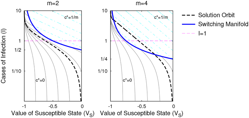
From Eq. (3.1a), we see S(t) = 0 for all t, which allows us to restrict our attention to the VS × I phase plane (see Figure 2). Eq. 3.1b is easily integrated by itself. When constructing solutions, we specify an arbitrary point (τ, S(τ), I(τ), VS(τ)) on the solution to identify constants of integration. The integrated form of solutions to Eq. 3.1c depends on the value of c*. If Ψ(I, VS) > 1/m, then c* = 1/m, dVS/dt = 1/m, we can calculate the system solution
| (3.2a) |
and when put in phase space form,
| (3.2b) |
Figure 2:
Phase plane for our solution orbits to the infinite-horizon problem when S = 0 under Eq. (1.6) for efficiencies m = 2 (left) and m = 4 (right). The thick black dashed line is the solution matching the terminal conditions, and is a lower bound on all solutions reaching the terminal value in finite time. The thick blue solid line is the switching surface where c* jumps from c = 0 (gray solid) to c = 1/m (cyan dot-dashed). Along the switching surface, the flow is not differentiable but is continuous and unique. When the efficiency is above e ≈ 2.718 (right), the Nash equilibrium response always incorporates social distancing for sufficiently large I(0), independent of the terminal time. When the efficiency is below the threshold (left), then for every I(0) > 0, there are terminal times T sufficiently large that social distancing is never optimal. A log scale has been used on the I axis for illustration purposes.
If Ψ(I, VS) < 1/m, then c* = 0, dVS/dt = (1 + VS)I, and
| (3.3) |
If Ψ(I, VS) = 1/m, we must consider the third possibility of singular trajectories along the switching surface. A singular equilibrium trajectory exists locally at a point if and only if the tangent space of the switching surface intersects the cone of feasible directions derived from the optimality conditions. Direct substitution of the switching condition into Eq. (3.1c) shows that when Ψ(I, VS) = 1/m, we must have , independent of c*. The vector field is tangent to the switching surface only at the isolated point (VS, I) = (1/m − 1, 1). So if S = 0, there are no singular trajectories. For any point on the switching surface where I < 1, solutions are entering the region where c* = 0 as time goes forward. For any point on the switching surface where I > 1, solutions are leaving this region and entering the c* = 1/m region.
To construct a complete solution of the infinite-horizon problem when S = 0, we need to find orbits solving the differential inclusion with terminal condition VS(∞) = I(∞) = 0 (see Figure 2). Clearly, Eq. (3.3) applies at this terminal time. Taking VS(τ) = I(τ) = 0, the terminal condition is matched by the orbit I(t) = − ln(VS(t) + 1). Running time backwards, the solution must flow along this orbit until it (possibly) intersects the switching surface. Whether or not it intersects the switching surface depends on whether there is a value of VS ∈ (−1, 0) that solves
| (3.4) |
We find that if m < e, there is no intersection – the game equilibrium strategy makes no use of social distancing and c*(t) = 0 for all t (see Figure 2, left). In this case, Eq. (3.3) fully specifies the solution. If m > e1, we can define two times t1 and t3 with t1 > t3 such that the first transition occurs at I(t1) which is the smallest solution of mIe−I = 1 (we will introduce t2 later in this paper). A second transition then occurs at I(t3), where I(t3) > I(t1) and
| (3.5) |
Explicit expressions for the switch-points can be obtained in terms of the principle branch Wp(x) of Lambert’s W function (Corless et al., 1996):
| (3.6) |
| (3.7) |
| (3.8) |
Between t1 and t3, the solutions are given by Eq. (3.2). No further patching occurs, as Ψ(I(t), VS(I(t))) < 1/m for all t < t3 (see Fig. 2, right). So the infinite-horizon equilibrium trajectory is completely determined.
Interestingly, since the epidemic dynamics are independent of behavior in this scenario, the game theory equilibrium must also correspond to the optimal control maximizing the well being of all individuals who are not infected.
4. Equilibria when some are susceptible (S > 0)
We now consider the infinite horizon problem when S > 0. Our governing system is again Eq. (1.3) with switching conditions given by Eq. (2.1a). If (c*, σ(c*)) = (1/m, 0), the trajectories satisfy Eq. (3.1) and are given by Eq. (3.2), with S(t) constant. On the other hand, if (c*, σ(c*)) = (0, 1),
| (4.1a) |
| (4.1b) |
| (4.1c) |
4.1. A necessary conditions for c* > 0.
If m < e, then c* = 0 along every equilibrium of the infinite-horizon problem. We know this because when c*(0, 0) = 0,
| (4.2) |
The right hand side is monotone strictly increasing in S. When we integrate backward in time from any terminal condition with 0 ≤ S(∞) < 1, we find that no trajectory – when collapsed from the S × I × VS phase space into the VS × I phase space – can cross the S = 0 equilibrium trajectory from Section 3. Since m < e implies the S = 0 trajectory takes c* = 0 everywhere, and larger values of S only make dI/dVS more positive, all equilibrium trajectories with S ≥ 0 must also do so. c* = 0 is the unique solution, because the strict monotonicity ensures Eq. (1.2) is always single-valued.
4.2. Equilibria not employing singular trajectories.
When m > e, equilibrium trajectories terminating in the neighborhood of S(∞) = 0 may intersect the switching surface, and we have to integrate explicitly to determine when the equilibrium trajectories include positive investments. The trajectories can be constructed in an implicit closed-form. Treating S as the independent variable,
| (4.3a) |
| (4.3b) |
Integrating through an arbitrary point (S(τ), I(τ), VS(τ)) and parameterizing the solution in terms of S(t),
| (4.4a) |
| (4.4b) |
| (4.4c) |
Alternatively, the solution may be parameterized in terms of V (t) by transforming Eq. (4.4b) to
| (4.5) |
and substituting as needed. There is no unique parameterization in terms of I(t), because Eq. 4.4a does not have a unique solution for S(t) in terms of I(t).
We now patch together solutions just as we did in Section 3. Tracing solutions backward in time from t = ∞, c* = 0 and the trajectory is given by System (4.4) until it hits the switching surface. At this point, c* = 1/m, and trajectories are given by System (3.2), with S constant. Over this region, Eq. (3.2b) holds.
Once they hit the switching surface a second time, which must occur for I > 1, we return to c* = 0, and trajectories are again given by System (4.4). There are never more than two discrete intersections between the equilibrium trajectory and the switching surface. When c* = 0, Eq. 4.2 implies that dI/dVS is monotone increasing in S, and hence bounded below by the S = 0 case:
| (4.6) |
The switching curve’s slope
| (4.7) |
which is more negative for any I > 1. Thus, as we integrate backward in time from any point on the switching curves with I > 1, the equilibrium trajectory can not re-intersect the switching curve.
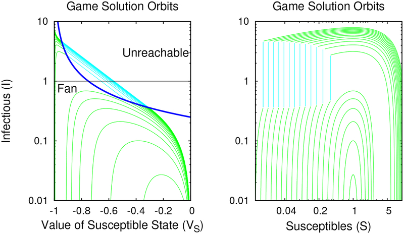
We can stop any place along the way, if the desired initial condition is reached. Figure 3 shows the trajectory orbits, as we can now construct them. We see that the solutions we have constructed can reach many initial conditions (S(0), I(0)), but there is a large gap, where certain initial conditions are not reached. However, we have not yet considered the possibility of singular trajectories when S > 0.
Figure 3:
Regular equilibria trajectories in VS × I phase space and S × I phase space for S(∞) ∈ [0, 1], I(∞) = V(∞) = 0, when σ(c) = max (1 − 4c, 0). The black curve from Fig. 2 corresponding to S = 0 is the least upper bound on the observed orbits; larger values of I for given VS are unreachable. Orbits passing through the gap labelled “Fan” exist, but must be constructed using singular controls. The absence of intersecting trajectories in S × I space which would represent shocks and folds will be indicative of a unique Nash equilibrium for the infinite-horizon initial-value problem.
4.3. A regional decomposition and singular trajectory construction.
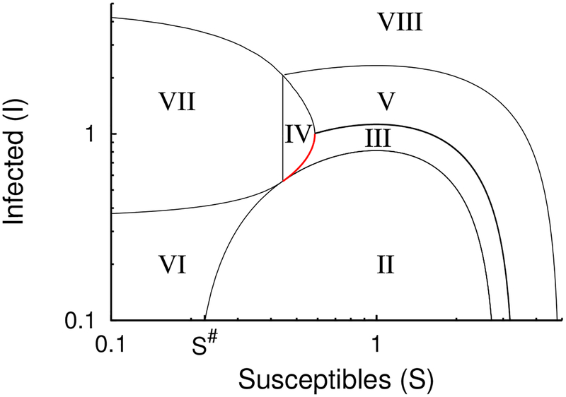
To fill this gap and ensure that there is a unique equilibrium trajectory for every initial condition in the infinite-horizon problem, it will be useful to decompose S × I state-space into closed regions, as in Figure 4, where the boundaries can be identified by the intersections of neighboring regions. Inside each of these regions, c is constant, so the Hamilton–Jacobi equation is linear and unique solutions exist, provided there are appropriate initial and boundary conditions. Consequently, the analysis will focus on the boundaries of the regions. To avoid notational confusion with our state variables, we start the region numbering at roman-numeral II.
Figure 4:
When the efficiency m > e, the S × I phase plane is dissected into eight regions that are used in establishing the existence and uniqueness of an infinite-horizon Nash equilibrium for all initial conditions. In region II, orbits are the elementary solutions of the SIR model. Region III is part of a fan originating from the afferent manifold. Region IV is the opposite side of the fan, where c* = 1/m. Region V extends region IV, with c* = 0. Region VI contains orbits which hit the switching surface. Region VII extends Region VI with c* = 1/m. Region VIII extends Region VII with c* = 0. Every initial condition S(0), I(0) lies in one of these regions or on their boundaries, and has a unique initial value VS(0) such that VS(∞) = 0.
First, let us define the closure of the set of all initial conditions (S(0), I(0)) for which c*(S(t), I(t)) = 0 for all times t > 0 and t < 0 as region II. The equilibria in II are constructed by solving System (4.4) for the given initial condition. When m < e, region II covers the whole non-negative quadrant. Region II is never empty, since for finite m we can always choose S(∞) close enough to 1 that I never becomes large enough to intersect the switching surface.
When m > e, the S = 0 solution in Section 3 shows that there is at least one region where c* is positive for intermediate times. Let us define region VI as the closure of the set of all initial conditions (S(0), I(0)) for which c*(S(t), I(t)) = 0 for all future times t > 0 but not already in region II. This means that for each initial condition in region VI, there is some t < 0 such that c*(S(t), I(t)) > 0. Let region VII be the set of all initial conditions starting with c*(S(0), I(0)) = 1/m and flowing into region VI, and let region VIII be the set of all initial conditions starting with c*(S(0), I(0)) = 0 and flowing into region VII. As long as m > e, we know that {0} × [0, I(t1)] ⊂ VI, {0} × [I(t1), I(t3)] ⊂ VII, and {0} × [I(t3), ∞) ⊂ VIII. We can also show by direct calculation that ([0, 1] × [0, 1/m])\II ⊂ VI
The boundary between regions II and VI, specified as II ∩ VI, is itself an orbit, and we would like to calculate this orbit. Let S#(m) := S(∞) for this specific orbit. The orbit must be tangent to the switching surface any place the two intersect. Let us re-interpret Ψ(S, I, VS) = I(VS + 1) as a potential, and observe that for any given m, the switching surface of our game is a level set of Ψ. Thus, the tangent space of the switching surface at any state can be represented as the space orthogonal to the gradient of Ψ. In particular, a trajectory moving tangent to the switching surface must satisfy
| (4.8) |
Substituting System (4.3) into (4.8),
| (4.9) |
which implies that tangency to the switching surface can only occur along
| (4.10) |
On the other hand, applying System (4.4) with terminal conditions I(∞) = 0, VS(∞) = 0, but free, equilibrium trajectories of the infinite-horizon problem have
| (4.11) |
Intersecting these 3 surfaces together with Eq. (2.2), we find that the tangent point must be given by
| (4.12) |
where satisfies
| (4.13) |
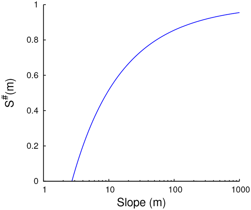
Eq. (4.13) has a unique positive solution for all m > e, and no solutions meeting our inequality conditions when m < e (see Figure 6). Based on the monotonicity results at the beginning of this section, if the terminal condition , then the trajectory never reaches the switching surface and c* = 0 everywhere, while if , then the trajectory passes through the switching surface and c* = 1/m for an interval. Thus, is the terminal condition of the orbit representing II ∩ VI.
Figure 6:
Graph of the solutions S#(m) of Eq. 4.13, depending on the slope m. There is no solution when m < e. Though the convergence rate is slow, limm→∞ S#(m) = 1.
For initial conditions in VI∪VII∪VIII, equilibria solutions always exist (by construction). They are also unique. The uniqueness of solutions depends on the shape of the boundary between VII and VIII. Suppose X1 and X2 are equilibria phase space trajectories for initial conditions in region VIII with X1.S(∞) < X2.S(∞)†. We see from the S × I phase portrait in Figure 3 that (X1 ∩ VI ∩ VII).S < (X2 ∩ VI ∩ VII).S and (X1 ∩ VI ∩ VII).I < (X2 ∩ VI ∩ VII).I. From the VS × I phase portrait in Figure 3, (X1 ∩ VI ∩ VII).I < (X2 ∩ VI ∩ VII).I implies (X1 ∩ VII ∩ VIII).I > (X2 ∩ VII ∩ VIII).I while (X1 ∩ VII ∩ VIII).S < (X2 ∩ VII ∩ VIII).S. These conditions ensure that X1 and X2 remain separate in region VIII as well as VII and VI.
When establishing connectivity of our regions, it will be very useful to make use of the “projection” of various sets by a vector field. Given a differential equation and two subsets A and T of a state space, we define the projection of A forward onto T under F as the intersection of T and the union of all positive-time half-orbits of with initial conditions in A. The backward projection of A onto T is defined analogously, but using the negative-time half-orbits.
To show that region VIII is simply connected and includes all but a compact subset of the S × I phase plane, we resort to continuity of solutions of differential equations in terms of the terminal conditions under projection. Both the S = 0 boundary of VI and VI ∩ II are equilibria trajectories. If we take the I = 0 segment between S = 0 and region II, and project it along the equilibrium trajectories using the differential equations and the terminal conditions, we know VI ∩ VII is a continuous curve touching S = 0 at one end and region II at the other. This, in turn, implies VII ∩ VIII is also a continuous curve touching S = 0 at one end. And from VII ∩ VIII, we can reach all initial conditions in VIII.
We can not, however, show by this argument that region II touches region VII and VIII. In fact, they do not touch each other – there is a gap of initial conditions that are not reached by this argument, as Figure 3 shows. We must now deal with this gap.
The only possibility remaining from Eq. (2.1a) is that there are trajectories in the switching surface where 0 < c*< 1/m. Substituting appropriate terms from Eq. (1.3) into Eq. (4.8), we find an equilibrium trajectory can track the switching surface only when c solves
| (4.14) |
Using σ’s definition in Eq. (1.6), we see that this is solved by
| (4.15) |
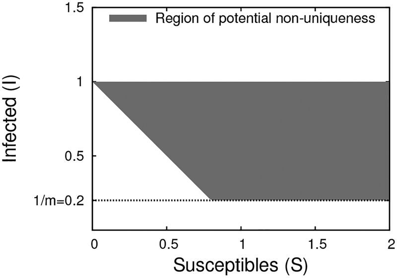
And since we must have , this can only hold as long as I ∈ [1 − S, 1], with c = 0 when I = 1 − S and c = 1/m when I = 1. This, combined with the earlier observation that the switching surface only exists when I ≥ 1/m, determines the subset of phase space where the differential inclusion may not be single-valued (see Figure 5).
Figure 5:
Region of state-space where the differential inclusion specified by Eq. (1.3) and (1.6) may be multivalued when m = 5. If (S, I) falls inside this region and I(1 + VS) = 1/m, the necessary condition only requires to be in the interval [0, 1/m]. Any singular equilibrium trajectory that tracks the switching surface must lie within the shaded region. Outside the shaded region, the necessary condition for is sufficient to uniquely determine integrated paths, even though itself is not everywhere uniquely determined. This applies for both infinite-horizon and finite-horizon analyses.
Eq. 4.15 can be differentiated to make a Riccati equation for the dynamics of ,
| (4.16) |
Integrating the evolution equations under these conditions, singular equilibrium trajectories lying within the switching surface have the form
| (4.17a) |
| (4.17b) |
| (4.17c) |
where (S(τ), I(τ)) is an undetermined contact point and Ψ(I(τ), VS(τ)) = 1/m. Now, to patch orbits, we need to identify where these singular equilibrium trajectories intersect the trajectories given by System (4.4) for some terminal conditions. Looking at Eq. (1.3) when c*= 0, we find that the differential inclusion can only flow into the switching surface when S + I ≤ 1 (independent of m). We show this by determining when c*= 0 implies the inner product
| (4.18) |
On the other hand, the singular equilibrium trajectories only satisfy the optimality conditions when S + I ≥ 1. Thus, any patching must occur along S + I = 1. By looking for an intersection between the solutions of System (4.4) and S + I = 1, we find that the only admissible point for (S(τ), I(τ), VS(τ)) is the tangent point of the orbit with terminal condition S#(m). Since S# only exists for m ≥ e, there are no singular trajectories for m < e.
The singular equilibrium trajectory we have constructed inside the switching surface is called an afferent manifold by Isaacs (1965) (see Figure 7). For positive S, the vector field (differential inclusion) along the afferent manifold is not outer continuous; not all elements of the cone at a given location are accumulation points of each sequence converging to that location. But the differential inclusion along the afferent manifold is contained in the union of accumulation cones of all convergent sequences (inner continuity)‡. This simplifies the analysis because it implies we need only consider the vector field at each point along the afferent manifold.
Figure 7:
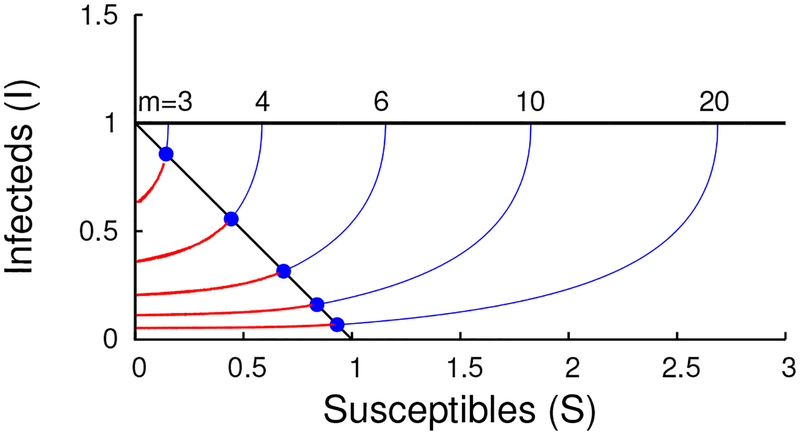
Construction of curves where infinite-horizon equilibrium trajectories intersect the switching surface for different efficiencies m in S × I state space. For values of S(∞) < S#(m) (red), the equilibrium passes directly through the switching surface, while for equilibria terminating with S(∞) = S#(m), the equilibrium trajectory can either remain in the switching surface on the afferent manifold (blue) or exit on either side. The line I = 1 − S (black) is the break between these two behaviors. Note that while Fig. 6 shows S#(m) increases slowly, this plot show that the intersection points with I = 1 − S increase more quickly. Curves for m = 3, 4, 6, 10, and 20.
4.4. Construction of equilibria using the afferent manifold.
The afferent manifold we have derived is a core from which we can fill in the gap in Figure 3 using a weak solution in the form of a fan (Kevorkian, 1990) (see Figure 8). We will show that this fan may reach every initial condition within our gap, and that no initial condition is reached by more than one equilibrium trajectory.
Figure 8:
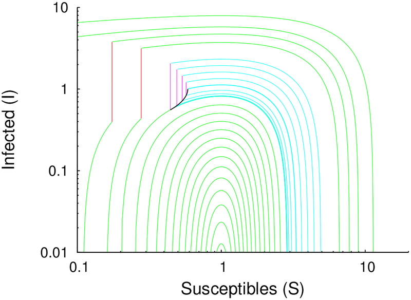
Construction of the complete set of equilibrium trajectories for the infinite horizon problem under Eq. (1.6) when m = 4. Green and cyan curves have c* = 0. Red and magenta curves have c* = ¼. the black curve at the center of the fan is the afferent manifold. The slight irregular spacing of the solutions is a consequence of sampling conditions chosen – a unique solution can be constructed to match any initial condition S(0), I(0).
Perturbing the afferent manifold to have Ψ(I, VS) > 1/m at each point, and then projecting the perturbed afferent manifold backward in time with c* = 1/m according to Eq. (3.1), the curve sweeps out regions IV and then region V where c* = 0. Since the afferent manifold originates at the intersection point II ∩ VI ∩ VII, region IV tightly abuts region VII, which in turn implies region V tightly abuts region VIII. The projection of the afferent manifold through IV does not re-intersect the afferent manifold because everywhere in the interior of region IV, while everywhere except at the terminal point of the singular trajectory when I = 1. Since the afferent manifold is continuous and the differential equations exhibit continuous dependence on their initial conditions in each of regions IV and V, the afferent manifold projection backward in time to form the boundary between regions IV and V is also continuous.
Perturbing the afferent manifold to a curve where Ψ(I, VS) < 1/m at each point, and then projecting the perturbed afferent manifold backward in time with c* = 0 according to Eq. (4.1), sweeps out region III. The boundary between region III and region II is formed by the trajectory terminating at S#, and since c* is constant in region III, each initial condition is reached by a unique path. Nor does the projection of the afferent manifold intersect the switching surface again, since Eq. (4.18) implies for all S + I > 1, I > 0, VS > −1. Since the terminal point of the afferent manifold at I = 1 is also in the boundary of region III, regions V and III must tightly abut each other.
Thus, all the regions abut each other tightly without overlap within or between regions. This leads us to the following conjecture.
Conjecture 1. When the relative exposure rate σ(c) is given by (1.6), then the infinite-horizon differential population game specified by (1.2), (1.3), and (1.4) has a unique subgame-perfect Nash equilibrium for any initial condition S(0), I(0).
I refer to this as a conjecture, rather than a theorem, because we have not paid careful attention to the messy details underlying this analysis but necessary in a formal proof. We have not, for instance, introduced the appropriate measure-theory tools needed to specify the equivalence classes in strategy-space, such that “uniqueness” makes sense. For instance, strategies may differ from the given strategy at isolated points without having any measurable effect on the solution. We have also been loose in our handling of issues of continuity of solutions, particularly at the boundaries of our solution regions.
Never the less, our analysis does appear sufficient for the calculation of a unique solution numerically. One complete example is shown in Figure 8. Some examples of regions of positive social distancing investments at Nash equilibrium for various efficiencies m are highlighted in Figure 9, along with the regions where singular trajectories may appear.
Figure 9:
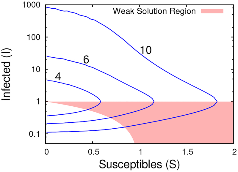
Boundaries of the regions of positive social distancing (c* > 0) for the equilibria of the infinite-horizon problem when σ(c) is given by Eq. (1.6) and the maximal efficiency of social distancing m ∈ {4, 6, 10}. The shaded region represents the portion of the state-space where singular controls are used to construct the equilibria.
5. Calculation of vaccine-deployment windows
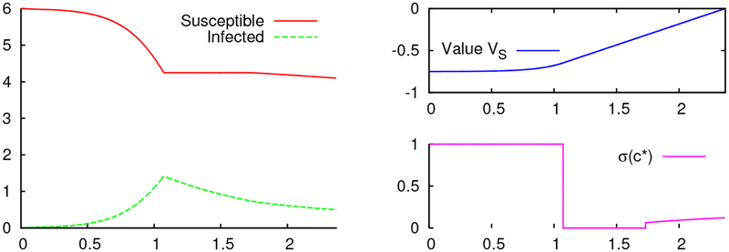
We now consider a finite planning horizon rather than an infinite planning horizon. Suppose a safe, effective, and free vaccine will become available to the entire population at a fixed time T after the start of the epidemic. This corresponds to a variant of our game with a finite-horizon and terminal condition VS(T) = 0. We will see that at equilibrium in this finite-horizon problem, the sequence of behaviors always fits the timeline shown in Figure 10: do nothing, do everything, do something, do nothing. To determine the equilibrium, we must calculate the times of each transition 0 ≤ t1 ≤ t2 ≤ t3 ≤ T, along with the exact investment rate between times t2 and t3. An example result is shown in Figure 11.
Figure 10:
This is a timeline of equilibrium investment c*(t) between the start of the epidemic at time 0 and the termination of the epidemic at time T when universal vaccination occurs. To determine the equilibrium, we must calculate the times of each of the transition 0 ≤ t1 ≤ t2 ≤ t3 ≤ T, along with the exact investment rate between times t2 and t3. In the case of S = 0, T = ∞, we always have t2 = t3, justifying the choice of notation in Section 3.
Figure 11:
An example time-series plot of the equilibrium trajectory to the finite-horizon problem calculated with S(0) = 6, I(0) = 0.01, m = 2, and T = 2.37. Panels show the state-variables S(t) and I(t) (left), along with the price of susceptibility VS(t) (top right), and the relative contact rate σ(c*) under the equilibrium control c*(t) (bottom right). In this case, 0 < t1 < t2 < t3 = T.
Let us construct a full equilibrium trajectory. Define V*(S(0), I(0)) as the value of the equilibrium trajectory of our infinite-horizon game at initial-condition (S(0), I(0)). Starting from an arbitrary initial condition (S(0), I(0), VS(0)), when I(0) ≈ 0, S(0) > 1 and 0 > VS(0) > V*(S(0), I(0)), we wish to determine T, where VS(T) = 0, along with any important intermediate times t1, t2, and t3. Our choices of a small I(0) will not cost us any generality because all larger values will lie along one of the equilibria we obtain. The surface formed by the union of all infinite-horizon equilibria trajectories forms a barrier, and trajectories diverge without ever reaching VS = 0 if the initial condition VS(0) < V*(S(0), I(0)).
We start by determining the time t1 of the first intersection between the trajectory and the switching surface. As long as I(0) < 1/m, the switching condition ensures t1 > 0 unless the terminal condition is reached first. The exact value of the t1 switch can be determined by enforcing Eq. (2.2), from which we expect
| (5.1) |
Using calculus, we can show that there may be no values of S(t1) that solve Eq. (5.1) when
| (5.2) |
Otherwise, there are two values of S(t1) that solve Eq. (5.1), or only a single solution in the degenerate case of equality. When there are two solutions, we can show that S(t1) must be the larger of the two, S(t1) ∈ [m(VS(0) + 1)S(0)/(mS(0)(VS(0) + 1) + 1), S(0)], with
| (5.3a) |
| (5.3b) |
and
| (5.3c) |
However, when there are no solutions to Eq. (5.1) then the trajectory reaches the terminal VS(T) = 0 before reaching the switching surface (T < t1), with
| (5.4a) |
| (5.4b) |
| (5.4c) |
Since is non-negative, VS can only cross the terminal condition once, and it suffices to test the endpoint t1. This also applies to each of the subsequent cases we are about to consider.
Let t2 be the time of the next transition when the trajectory again hits the switching surface. If I(t1) < 1, then we are already on the lower side and we can take t2 = t1. Otherwise,
| (5.5a) |
| (5.5b) |
| (5.5c) |
| (5.5d) |
This can be solved for t2 − t1 using scalar root-finding. Again, the terminal condition could be reached before the second switch. If VS(t2) > 0, then we have progressed too far, and define
| (5.6) |
There are now two more possibilities – the solution may pass immediately through the switching surface, or may track the switching surface for some time. Define t3 as the time when the trajectory leaves the switching surface. If S(t2) + I(t2) ≤ 1, then t3 = t2. Otherwise, solutions hitting the switching surface a second time must track it until they reach S(t3) + I(t3) = 1 or VS = 0. If S(t3) + I(t3) = 1,
| (5.7a) |
| (5.7b) |
| (5.7c) |
| (5.7d) |
These can again be solved with scalar root-finding. If VS(t3) > 0, then we have gone too far and define T < t3. When VS(T) = 0, we will have I(T) = 1/m. Within the switching surface, , so I(T) = I(τ)/(1 + (t − τ)I(τ)). Substituting and solving for t3 = T,
| (5.8a) |
| (5.8b) |
Finally, if we have left the switching surface with VS(t3) < 0, then we look for the final time T > t3, with V(T) = 0,
| (5.9a) |
| (5.9b) |
| (5.9c) |
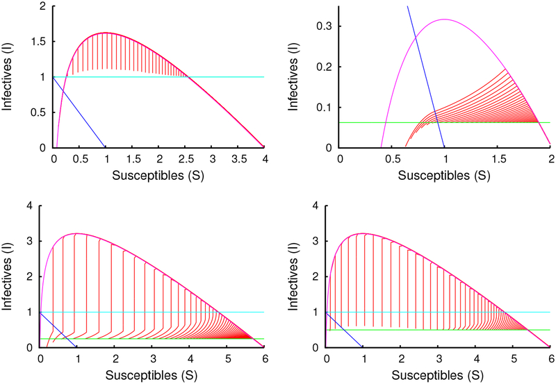
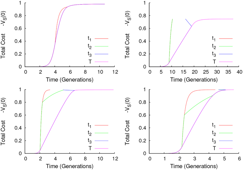
Having determined the states at times t1, t2, t3, and T, we can construct the full trajectories by quadrature (see Figure 12). From this process, we can determine a value of T for each initial choice of VS(0) between 0 and the infinite-horizon value V*(S(0), I(0)). Examples are shown in Figure 13.
Figure 12:
Varieties of phase plane orbits for finite-time solutions for a range of initial expected values V (0) when I(0) ≈ 0. All numerical evidence indicates that final time T increases as the initial cost increases, which would imply uniqueness. Parameter values: S(0) = 4, m = 1 (top left), S(0) = 2, m = 16 (top right), S(0) = 6, m = 4 (bottom left), S(0) = 6, m = 2 (bottom right).
Figure 13:
This presents plots of the strategy change-times t1, t2, t3 and T for the finite-time problem as the total cost VS(0) varies when , m = 1 (top left), , m = 16 (top right), , m = 4 (bottom left), or , m = 2 (bottom right). Total distancing (t1 ≠ t2) is only used when vaccine deployment is very late. For faster deployment, Nash equilibrium makes use of managed distancing, where risks are perfectly balanced. For much of the range, the cost grows linearly with increases in delivery time. Conjecture 2 is supported by the observation that the T-curves appear to specify bijections between VS(0) and the terminal time.
The per-capita cost of the epidemic as a function of the time to mass-vaccination when everybody acts according to the equilibrium strategy is approximated by
| (5.10) |
Changes in the efficiency m seem to principally affect how soon the region of active social distancing is reached and the amount of time spent on the switching surface. The durations of all other parts of the trajectory seem less sensitive to the efficiency.
We also see that the finite-horizon game can exhibit social distancing even when the efficiency is to low to be useful in the infinite-horizon game. Assume (S(0), I(0)) is inside region III, V, or VIII. If social distancing is efficient and m > m#, then for all sufficiently large deployment windows, t1 < t3. The infinite-horizon game equilibrium uses no social distancing if m < m#. But if m < m#, then there is a finite time window for T, where t1 < t3 = T and t1 < t < t3 implies cs(t) > 0. This only hold for some intermediate window of durations – if the window is to short or too long, then t1 = t3 = T.
It appears that T(VS(0)) is monotone increasing, with T(V*(S(0), I(0))) = ∞ and T(0) = 0, implying that for each vaccination window, there is a unique solution of our boundary-value problem with that duration. While we are able to construct these finite-time trajectories forward in time from a particular initial condition (S(0), I(0), V(0)) to a terminal condition V(T) = 0, thereby determining T, and then are able to use efficient numerical methods to determine which V(0) maps to the desired window length, we have not yet established that this relationship is a bijection. Instead, this is left as a conjecture whose proof will need some careful bookkeeping.
Conjecture 2. The finite-horizon differential population game of social distancing during an epidemic with σ(c) = max {0, 1 – mc} has a unique Nash equilibrium.
In lieu of a proof, this condition can be checked numerically on a case-by-case basis.
6. Discussion
In this paper, we have provided a detailed analysis of the differential population game equilibrium of social distancing during an SIR epidemic when the relative exposure rate is linear in e ort with zero-lower-bound. We provide methods for constructing these equilibria in infinite-horizon and finite-horizon problems, and show that the solution of the infinite-horizon problem is unique. In both cases, we make use of fans connected to an afferent manifold to fill in the full solutions for intermediate conditions. In many ways, the solution speaks for itself. Uniqueness of equilibria to the finite-time case is only conjectured. Another related general conjecture suggested strongly by comparison of Figures 2 and 3 is that the value of the susceptible state is always less than the value of the susceptible state when S = 0 – removing susceptible individuals always improves the value of the susceptible state, but only so-far. Our analysis was conducted in the absence of any discounting, under the assumption that epidemics are fast relative to economic and demographic processes. If we were to include discounting, it’s effect would be to diminish expected future costs associated with infection. This, it turn would probably diminish the amount of social distancing used at equilibrium, and delay the start of social distancing.
Our early assumption that social distancing alters exposure rates per contact but not the number of contacts is an assumption that facilitates our mathematical analysis, but is not necessarily universal. In many other epidemic theories, contact rates are positively correlated to effective population size, and social distancing through self quarantine may be viewed as reducing the effective population size. The simplest such example would be a standard incidence model (Auld, 2003), with
| (6.1a) |
| (6.1b) |
This model should be amenable to analysis similar to that presented above, although with more complicated algebra. In particular, the infection pressure remains a monotone decreasing function of c in this case. More general dependences of contact-rate will probably not be amenable to our analysis when they lack a first-integral. Numerically, there does not appear any reason to expect qualitative differences in the solutions for these cases compared to the current case. However, recent research (Chen et al., 2011; Chen, 2012) indicates that multiple steady-state Nash equilibria can appear under alternative hypotheses on contact pattern. If a contact pattern allows multiple steady-state equilibria, it seems unlikely that our uniqueness results will continue to hold, and there may not even exist a pure-strategy game equilibrium. Further analysis is needed.
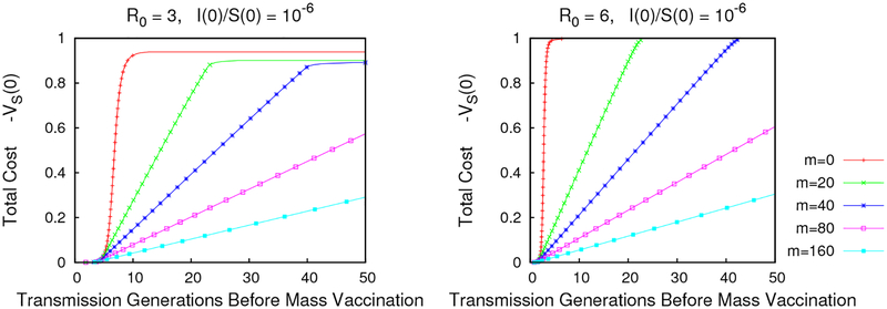
The form of σ(c) we have considered here is the weakest form satisfying the conditions that σ be positive, monotone decreasing, and convex – each of these conditions is only weakly satisfied. One consequence is that the windows of opportunity calculated with this model provide upper bounds on the window sizes for all other positive, monotone-decreasing, convex σ. Figure 14 provides some example calculations of window duration. These windows are significantly larger than those previously calculated in Reluga (2010) when σ(c) = 1/(1 + mc) for comparable values of m. This suggests that window lengths are sensitive to the tail-shape of σ, and that for applications we should be careful about determining its asymptotic properties.
Figure 14:
Windows of Opportunity for Vaccination. Plots of how the net expected loss per individual depends on the amount of time until mass vaccination when (left) and (right) . The windows are much longer than those found by Reluga (2010) for similar parameter values but σ = 1/(1 + mc), suggesting that equilibrium behaviors are sensitive to the shape of the tails of σ.
The closely related optimal-control problem of determining the best social-distancing rates in a cooperative population (Reluga, 2010) has not yet been considered, but is expected to have qualitatively similar features to the results presented here, including a fan for intermediate initial population sizes.
The success of the analysis presented here suggests some approaches for the general problem. In particular, the set Σ of all non-negative, decreasing, and convex functions σ(c) with σ(0) = 1 is the closure of the set of all piecewise linear functions of the form
So solution of a large-enough set of piecewise linear functions may lead to the general determination of existence and uniqueness. Among the many results possible, we can pose the following conjecture.
Conjecture 3. If
then for every initial condition S(0), I(0) and terminal condition VS(T) = 0, there is a unique equilibrium strategy c* to System (1.2)–(1.4).
Unfortunately, the solutions for these σ(c)’s can probably not be obtained in closed form; in any region where c* is constant and c* > 0 while σ(c*) > 0, the integration for VS(t) does not have an efficient closed-form representation. Without a closed-form representation, results will be less complete than those provided here. Yet this approach may still be fruitful in addressing the problem of uniqueness. Alternatively, approaches based on the Hamilton–Jacobi equation
| (6.2) |
may also provide general results for existence and uniqueness.
The differential population game of social distancing during an SIR epidemic is perhaps the simplest formulation which will allow us to study the time-dependent nature of social distancing during an epidemic. It has many short-comings. To begin with, the SIR epidemic model does not accurately describe the dynamics of any particularly disease, and many authors have published improvements motivated by particular applications. A second issue is that different types of social distancing may alter the epidemic dynamics in different ways, and the elasticity of the transmission network in response to individuals’ behavior changes can influence disease dynamics (Chen, 2012). A third issue is that there is a complete absence of any mechanistic representation of logistical issues like vaccine or antiviral allocation. These are issues to be considered as part of future research.
Acknowledgments
I am grateful to the reviewers for their diligence and helpful comments. This research was partially supported by NSF grant DMS-0920822, NIH grant PAR-08–224, and Bill and Melinda Gates Foundation Grant 49276.
Footnotes
Here X.S is used to indicate the S component of a position vector X. This notation is the same as that used commonly in object oriented computer languages and will make our analysis more readable than the use of arbitrary vector indices.
Within the literature on correspondences, the terms upper semicontinuity and upper hemicontinuity are used as synonyms for outer continuity, while lower semicontinuity and lower hemicontinuity are used as synonyms for inner continuity. These terms have various draw-backs that the inner–outer dichotomy avoids.
References
- Arrow KJ and Kurz M (1970). Public Investment, the Rate of Return, and Optimal Fiscal Policy. Baltimore, MD: Johns Hopkins Press. [Google Scholar]
- Auld M (2003). Choices, beliefs, and infectious disease dynamics. Journal of Health Economics 22, 361–377. [DOI] [PubMed] [Google Scholar]
- Bressan A and Piccoli B (2007). Introduction to the Mathematical Theory of Control. American Institute of Mathematical Sciences. [Google Scholar]
- Chen F (2012). A mathematical analysis of public avoidance behavior during epidemics using game theory. Journal of Theoretical Biology 302, 18–28. doi: 10.1016/j.jtbi.2012.03.002. [DOI] [PubMed] [Google Scholar]
- Chen F, Jiang M, Rabidoux S and Robinson S (2011). Public avoidance and epidemics: Insights from an economic model. Journal of Theoretical Biology 278, 107–119. doi: 10.1016/j.jtbi.2011.03.007. [DOI] [PubMed] [Google Scholar]
- Clark CW (1976). Mathematical Bioeconomics. John Wiley & Sons; New York. [Google Scholar]
- Corless RM, Gonnet GH, Hare DEG, Jeffrey DJ and Knuth DE (1996). On the Lambert W function. Advances in Computational Mathematics 5, 329–359. doi: 10.1007/BF02124750. [DOI] [Google Scholar]
- Fudenberg D and Tirole J (1991). Game Theory. MIT Press. [Google Scholar]
- Isaacs R (1965). Differential Games: A mathematical theory with applications to warfare and pursuit, control and optimization. New York: John Wiley and Sons. [Google Scholar]
- Kermack WO and McKendrick AG (1927). Contributions to the mathematical-theory of epidemics. Proceedings of the Royal Society of London 115, 700–721. [Google Scholar]
- Kevorkian J (1990). Partial Differential Equations: Analytic Solution Techniques. London, UK: Chapman & Hall. [Google Scholar]
- Lenhart S and Workman JT (2007). Optimal Control Applied to Biological Models. Chapman & Hall/CRC. [Google Scholar]
- Reluga TC (2010). Game theory of social distancing in response to an epidemic. PLoS Computational Biology 6, e1000793. doi: 10.1371/journal.pcbi.1000793. [DOI] [PMC free article] [PubMed] [Google Scholar]
- Reluga TC and Galvani AP (2011). A general approach for population games with application to vaccination. Mathematical Biosciences 230, 67–78. doi: 10.1016/j.mbs.2011.01.003. [DOI] [PMC free article] [PubMed] [Google Scholar]
- Sandholm W (2011). Population games and evolutionary dynamics. Cambridge, MA: MIT press. [Google Scholar]


