Individualization of Ultrafiltration in Hemodialysis

Abstract

Objectives:

There are approximately 660,000 end-stage renal disease (ESRD) patients in the USA, with hemodialysis (HD) the primary form of treatment. High ultrafiltration rates (UFRs) are associated with intradialytic hypotension, a complication associated with adverse clinical outcomes including mortality. Individualized UFR profiles could reduce the incidence of intradialytic hypotension.

Methods:

The patient’s fluid dynamics during HD is described by a nonlinear model comprising intravascular and interstitial pools, whose parameters are given by the patient’s estimated nominal parameter values with uncertainty ranges; the output measurement is hematocrit. We design UFR profiles that minimize the maximal UFR needed to remove a prescribed volume of fluid within a set time, with hematocrit not exceeding a specified time-varying critical profile.

Results:

We present a novel approach to designing individualized UFR profiles, and give theoretical results guaranteeing that the system remains within a pre-defined physiologically plausible region and does not exceed a specified time-invariant critical hematocrit level for all parameters in the uncertainty ranges. We test the performance of our design using a real patient data example. The designed UFR maintains the system below a time-varying critical hematocrit profile in the example.

Conclusion:

Theoretical results and simulations show that our designed UFR profiles can remove the target amount of fluid in a given time period while keeping the hematocrit below a specified critical profile.

Significance:

Individualization of UFR profiles is now feasible using current HD technology and may reduce the incidence of intradialytic hypotension.

I. Introduction

IN the United States, approximately 660,000 individuals have ESRD, with 468,000 on dialysis and 193,000 live with a kidney transplant [1]. The dominant modality of dialysis is thrice-weekly hemodialysis (HD) to remove waste products from blood and remove excess fluid by ultrafiltration (UF). Depending on the definition used, intradialytic hypotension (IDH) – significant drop in blood pressure – occurs in up to 30% of HD sessions [2]. IDH is mainly caused by imbalance between the ultrafiltration rate (UFR) and the refilling rate from the interstitial space, resulting in a reduction in absolute blood volume. IDH presents as nausea, muscle cramps, fainting, and anxiety. Symptomatic hypotension during HD requires immediate intervention, which includes reducing or stopping UF, administering fluid, and medication. IDH results in dyspnea, fatigue, cognitive impairment, and other indications negatively affecting quality of life [3]. In addition, IDH episodes and missed treatments due to related hospitalizations reduce the effectiveness of HD. IDH is associated with increased cardiovascular morbidity and mortality with a 10-20 fold increased risk [4].

There are multiple challenges to maintaining stable hemodynamics in patients on dialysis. Firstly, dry weight (DW), the euvolemic body weight for the patient, is only an estimate by the clinician and when objectively evaluated is often too high or too low [5]. Secondly, dialysis has been shown to lead to myocardial “stunning”, which will interfere with achievement of DW without hypotension and/or other symptoms [6]. Thirdly, uremia leads to dysfunction of the cardiovascular and autonomic nervous system response at many levels [7]. Lastly, many of these patients have severe comorbidities, such as cardiac disease, arterial “stiffness,” neuropathy, that also interfere with a normal hemodynamic response to fluid removal [8]. Thus it is unlikely that clinicians can prescribe a fluid removal pattern that can adjust for these variables based only on clinical experience.

The single most important measurement available to clinicians for guiding fluid removal during HD is blood pressure (BP). In subjects with healthy kidneys, autonomic and cardiovascular adaptations maintain BP necessary for adequate organ perfusion in the face of varying blood volumes [9]. However, the current practice of measuring BP every 20-30 minutes during HD cannot predict an IDH event, given that BP is tightly regulated by several intrinsic control mechanisms that respond to UF-induced blood volume reduction on time scales ranging from seconds to minutes. When the rate of microvascular refilling is smaller than UFR, plasma volume may decline to levels leading to hemodynamic instability and IDH. Therefore, it is essential that, in addition to BP, routine HD treatments include blood volume monitoring [10].

Sensors integrated in dialysis machines are able to track in real time the concentration of various blood components, such as protein water concentration and hematocrit (HCT), with high accuracy and resolution, and to derive relative blood volume (RBV) changes [11–13]. In the USA, the Crit-Line monitor [14] is the only available HCT sensor. Several studies used this sensor to explore a critical hematocrit level beyond which IDH could be expected – the so-called “crash crit”. RBV or HCT trends during HD were used for real-time UFR changes as hematocrit approached its critical level, but with inconsistent results [15–17]. A recent study derived target RBV levels at different HD treatment times that are associated with lower all-cause mortality [18].

Recent focus on fluid management has shifted to the adverse effect of higher UFR levels on cardiovascular morbidity and mortality. Several large retrospective studies have shown that rates over 13 ml/hr/kg were significantly associated with greater risk of all-cause and cardiovascular death compared with rates below 10 ml/hr/kg [4]. Consequently, the Centers for Medicare and Medicaid Services is considering a limit on UFR level as a quality measure for the ESRD Quality Incentive Program [19].

The application of feedback control systems to regulate UF by monitoring RBV, heart rate, and BP has been described in [20–23]. For example, [20, 23] describe multivariable biofeed-back systems which adjust UFR by monitoring the change in RBV and heart rate by tracking a pre-defined reference trajectory of relative blood volume to avoid an abrupt change in blood volume that may trigger IDH. This algorithm cannot guarantee that the required volume can be removed nor does it minimizes maximal UFR level. Generally speaking, these methods do not offer robustness with respect to physiological parameter variability in HD patients [24, 25].

It is apparent that in spite of major technical advances in HD technology the incidence of IDH is still high. This can be attributed to the high inter-patient variability in the hemodynamic response to UF. As a result, existing population-based UFR profiles are effective only in subsets of HD patients. Stakeholders have recently called for making fluid management a central concern in HD treatments [8].

Motivated by the above concerns, we present a new approach for the design of individualized UFR profiles that reduce UFR levels and manage hematocrit levels during HD for a patient model. In this approach, for a fluid dynamics model estimated for an individual patient, we minimize the maximal UFR needed to remove a prescribed volume of fluid within a prescribed time, subject to a time-varying critical hematocrit constraint. The underlying fluid dynamics during HD is described by a nonlinear fluid-volume model presented in the next section. We present a result that guarantees that the nonlinear system remains within a pre-defined physiological region and satisfies a (time-invariant) hematocrit constraint. Simulations suggest that time-varying hematocrit constraints are also satisfied. We demonstrate the perfonnance of our approach through a simulation example using a set of parameters based on clinical data.

The paper is organized as follows. Section II presents a non-linear, two-compartment model describing the fluid dynamics between the intravascular and interstitial volumes during UF. Section III describes our profile design based on a linearized model and Section IV analyzes this design when applied to the nonlinear system. Section V provides an example of our approach, and conclusions are made in Section VI.

II. Nonlinear, Two-Compartment Model of Fluid Volume Dynamics

Following [26–28], we model only the extracellular fluid dynamics during HD by assuming negligible fluid exchange with the intracellular compartment [29]. The extracellular fluid is modeled by two compartments, intravascular (plasma) and interstitial pools separated by a capillary membrane wall (see Fig. 1). Our model also includes the lymphatic system which returns a small amount of fluid and proteins from the interstitial compartment into the intravascular compartment. We model UF as fluid removed from the intravascular compartment during HD. Throughout this paper, we apply our results to a patient model estimated from clinical data (see [26–28] for more details).

Fig. 1.

Diagram of two-compartment fluid model.

The fluid dynamics of this model is described by the nonlinear differential equations

$$\begin{gathered} {\dot{x}}_1=R\left(x\right)-u \\ {\dot{x}}_2=-R\left(x\right) \\ Hct=\frac{V_{rbc}}{V_{rbc}+x_1} \end{gathered}$$ (1)

where x = (x₁, x₂) is the fluid state of the system, x₁ and x₂ represent the volumes of the intravascular and interstitial compartments respectively, input u is the UFR, and output Hct is the measured hematocrit which increases with the red blood cell volume V_rbc and varies inversely to x₁. The rate R(x) represents the net flow between compartments comprising lymphatic and microvascular flows. This rate is a nonlinear function of the fluid state x and primarily depends on five parameters V_rbc, K_f, f, d, and m_p as described in Appendix A. The nominal parameters used in this paper are based on an illustrative example of UF of clinical data set shown in Fig. 2. Parameter identification is based on the first 30 minutes of the HD session. We observe a good agreement between the simulated response (estimated model driven by clinical UF) and the average clinical response (the noisy measurement is a characteristic of the sensor). Further description of our identification approach can be found elsewhere [27, 28].

Fig. 2.

An illustrative example of a UF clinical data set; Top: the UFR profile used to remove 2 L within 3.42 hrs, Bottom: the resulting HCT (solid) and modelled HCT (dotted).

To allow for estimation errors we put uncertainty ranges around each of the parameters p in Table I. For simplicity we used a ±15% “spread” around the estimated value $\widehat{p}$ of p, thus $\widehat{p}\pm 0.15\times \widehat{p}$. This was guided by the size of 90% confidence intervals (CIs), $\widehat{p}\pm 1.645SE\left(\widehat{p}\right)$ where $SE\left(\widehat{p}\right)$ is the standard error of $\widehat{p}$ obtained from clinical data. The choice of 15% had the result that the uncertainty ranges contain the 90% CIs for K_f, V_rbc, and m_p, and almost coincide with those for d and f. Uncertainty ranges can be tailored more precisely to individual parameters, but as it was not the main concern of this paper we did not pursue this further.

TABLE I.

Individualized Model Parameters and Uncertainty Ranges

Parameter	Nominal	SE	Uncertainty range
Kf [L/min*mmHg]	0.0055	2.9e-4	[0.0047, 0.0063]
Vrbc [L]	1.0522	0.058	[0.8944, 1.21]
d [dimensionless]	0.01	0.001048	[0.0085, 0.0115]
f [dimensionless]	1.4	0.17178	[1.19, 1.61]
mp [g]	210	1.491	[178.5, 241.5]

III. UFR Profile Design

In this section we design a UFR profile u to meet the following objectives:

1. remove a specified amount of fluid in a given amount of time;

2. satisfy a given, time-dependent, upper-bound on hematocrit (i.e., critical hematocrit profile);

3. minimize the maximum ∥u∥_∞;

4. guarantee the above objectives over the parameter ranges in Table I.

The first objective is self-evident; the second provides an implicit lower bound to plasma volume to avoid hypotension and is feasible since HD machines typically integrate real-time hematocrit sensors such as Crit-Line [14]; the third objective aims to avoid the adverse effects associated with removing too much fluid too quickly; and the last guarantees performance in spite of parameter estimation errors.

The nonlinear compartment model (1) taken over the range of parameters in Table I constitutes a family of models. Our goal is to design a single UFR profile that meets the above specifications when applied to each model in this family. For the tractability of this design process we linearize and discretize these nonlinear models to produce a corresponding family of linear, discrete-time systems. The associated sampling period is T minutes over which the UFR profile is piecewise constant and has duration of nT minutes. From Appendix B, this family of linear systems is described by the difference equation

$$Hc{t}_k=Hc{t}_0+{\theta }_3\sum _{i=0}^{k-1}{u}_i+{\theta }_2\sum _{i=0}^{k-1}{\theta }_1^{\left(k-1-i\right)}{u}_i$$ (2)

where k = 1, …, n, Hct₀ is the initial hematocrit, u_k denotes u(kT), and where the parameters θ₁, θ₂, and θ₃, accounting for the model parameter uncertainty described in Table I, take on values in the ranges 0.8868 ≤ θ₁ ≤ 0.9617, 0.0394 ≤ θ₂ ≤ 0.0523, and 0.0014 ≤ θ₃ ≤ 0.0091. The mapping between the set of primary parameter vectors (V_rbc, d, f, K_f, m_p) allowed by Table I and the discrete-time parameters θ = (θ_t, θ₂, θ₃) is given by equations (B.6) and (B.8). The set of all possible combinations of θ in the above intervals yields the set of vectors ϴ = [0.8868, 0.9617] × [0.0394, 0.0523] × [0.0014, 0.0091]. The set ϴ is “larger” than the set of primary parameters; i.e., there are discrete-time parameters in ϴ having no corresponding primary parameters in the ranges of Table I. We now design a suitable UFR profile for this linear family of models.

We pose the UFR design as the solution to the following linear program:

$$\begin{array}{ll}\underset{u_k,\overline{u}}{\mathrm{minimize}}& \overline{u}\\ \mathrm{subject}\mathrm{to}& 0\le u_k\le \overline{u}\\ & 0<\overline{u}\le u_{max}\\ & 0.95V_T\le T\sum _{k=0}^{n-1}{u}_k\le V_T\\ & \underset{\theta \in \Theta }{\max }Hc{t}_k\le Hc{t}_{c,k}\end{array}$$ (3)

The first constraint limits UFRs to be less than some maximal value $\stackrel{‒}{u}$ which itself has a given clinical bound u_max imposed by the second constraint. The third constraint guarantees at least 95% of target volume of plasma V_T will be removed (a clinically negligible relaxation to avoid program infeasibility) while the last constraint guarantees that a given critical hematocrit profile Hct_c,k is never exceeded over all model parameters θ. The maximization of Hct_k in the last constraint is achieved for all k when the components of θ take on their largest values, (0.9617, 0.0523, 0.0091). This property holds for all individuals and relies on the structure of the linearized system (2) and ϴ being a rectangular box - though, as previously mentioned, these maximizing θ_i’s may not have corresponding primary parameters in the ranges of Table I.

In Section V we will provide an example to illustrate this UFR design process. Next we analyze the response of the original nonlinear system (1) to the UFR profile designed using the present method.

IV. Behavior of the Nonlinear System Under the Designed UFR Profile

The UFR profile u_k produced in Section III is based on a simplified model, i.e., a linearized version of (1), sampled at time intervals of length T. Applying a zero-order hold (ZOH) to u_k we obtain the continuous-time profile u(t), t ≥ 0, which is to be used in the dialysis setting. The performance of u_k is guaranteed only for the simplified model, whereas u(t) must be applied to the “full” nonlinear, continuous-time model (1). In this section we show that, under conditions that can be easily checked in practice, two requisite clinical conditions will be satisfied: (i) the target amount of fluid (within 5%) will be withdrawn during the given dialysis period, and (ii) the hematocrit will be kept below a (time-invariant) specified critical value. Condition (ii) is the more difficult to establish. Notice that, from (1), keeping HCT below a critical value corresponds to keeping the plasma volume x₁ above a “critical” value.

Although we have not been able to prove it analytically, our experience with many examples shows that u_k is a monotone non-increasing sequence, u_k ≥ u_k+1, and so u(t) will be monotone non-increasing. We shall, however, establish our results for an arbitrary sequence u_k ≥ 0, not necessarily the one from section III, and with a continuous-time UFR profile u(t) related to the sequence as we now describe. We always assume that continuous-time profiles u(t) are right-continuous and nonnegative. Given a subinterval [t₀, t₁) of [0, t_f], where t_f > 0 is the duration of the dialysis session, the profile u(t) is said to depend from (in the sense of “hang down from”) u(t₀) if u(t) ≤ u(t₀) ∀t ∈ [t₀, t₁). A set of times 0 = T₀ < T₁ < … < T_n = t_f is called a partition of [0, t_f], and we say that the profile u(t) is attached to the partition and the sequence u_k if u(T_k−1) = u_k and u(t) depends from u_k on [T_k−1, T_k), k = 1 … n. Our designed profile u(t) is defined by ZOH applied to the sequence u_k obtained in section III; thus u(t) is attached to the partition T_k = kT and that sequence. A monotone nonincreasing profile u(t) will be attached to any partition and the sequence u(T_k).

For any UFR profile u(t), let $U\left(t\right)\equiv {\int }_0^{t}u\left(\tau \right)d\tau$ be the amount of fluid removed during the time interval [0, t]. If u(t) is derived from a sequence u_k by ZOH, then $U\left(nT\right)=T{\Sigma }_0^{n-1}{u}_k$, thus, 0.95V_T ≤ U(nT) ≤ V_T if the third condition in (3) is satisfied, whence assertion (i) is proven.

Let B₀ be the set of points in the open first quadrant where the function R(x) is well-defined, as described in detail in Appendix A. Let E₀ be the set of equilibrium points of (1) within B₀ when the UFR is “turned off”, i.e., u(t) ≡ 0, E₀ = {x ∈ B₀ : R(x) = 0}. Due to the nonlinearity of R(x), E₀ has to be evaluated numerically. As shown in Appendix C, E₀ is the graph of a differentiable, monotone increasing continuous function that “cuts” B₀ into two regions, i.e., where R > 0 and R < 0. The discussion in Appendix A shows that R(x) is continuous in B₀ and the partial derivatives satisfy R₁ ≐ ∂R/∂x₁ < 0 and R₂ ≐ ∂R/∂x₂ > 0. Next, choose a rectangle B = [x_1L, x_1H] × [x_2L, x_2H] contained in B₀ with lower left corner (x_1L, x_2L) and upper right corner (x_1H, x_2H) both in E₀. Thus E₀ cuts B from the “southwest” corner to the “northeast” corner into two regions, the vascular refilling region, E⁺ ≐ {x ∈ B : R(x) > 0}, and the region of vascular flow into the interstitial compartment, E⁻ ≐ {x ∈ B : R(x) < 0}. The situation is illustrated in Fig. 4. In what follows we shall write E_v ≐ {x ∈ B : R(x) = v}, including for v = 0. The dependence of the function R(x) and associated sets E₀, etc., on the vector of “primary” parameters, p = (V_rbc, d, f, K_f, m_p) is suppressed from the notation; likewise for the solution x(t) of (1). The results below pertain to an arbitrary but fixed value of p in the range determined by Table I.

Fig. 4.

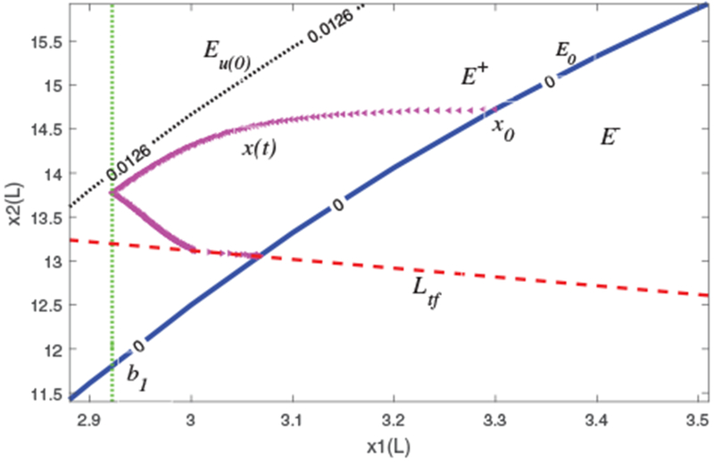
State-space response of (1): trajectory x (triangle) remains in physiological set B = [2.88, 3.51] × [11.4, 15.92], and satisfies a minimal critical plasma volume constraint b₁ (dotted, vertical). Notation: E₀ (solid) and E_u(0) (dotted), L_tf (dashed).

Let x(t) be a solution of (1) with initial condition x₀ = (x₁₀, x₂₀), and with u(t) ≥ 0, 0 ≤ t ≤ t_f, an arbitrary UFR profile. Let V(t) = x₁(t) + x₂(t), the total fluid volume in the system at time t. We define r(t) ≡ R(x(t)), the flow rate into the vascular compartment at time t, and r_i(t) = R_i(x(t)), i = 1, 2. The following are our main results for the full nonlinear system under the designed UFR profile (see proofs in Appendix D). They are actually somewhat more general as they do not use any properties of R(x) beyond those in the previous paragraph and they hold for a large class of UFR profiles. Theorem 1 shows that, under appropriate initial conditions, solutions x(t) of the full model (1) remain within a physiologically reasonable region.

Lemma 1. Suppose r(t₀) = v > 0 for some t₀ ∈ [0, t_f] and that u(t) ≤ v for t ≥ t₀. Then r(t) ≤ v for t ≤ t₀.

Theorem 1. Assume u(t) ≤ u(0)) for all t in [0, t_f]. Let a_2L be the solution of R(x_1L, a_2L) = u(0) and assume U(t_f) < V(0) − (x_1L + a_2L). Let x(t) be a solution of (1) with x₀ ∈ B.

a) If 0 ≤ R(x₀) ≤ u(0), then, for 0 < t ≤ t_f, x(t) stays in the region C_r ⊂ B bounded by E_u(0), E₀, and the line L_tf having slope −1 and x₁–intercept V(0) − U(t_f).

b) If R(x₀) > u(0), then x(t) ∈ B for 0 < t ≤ t_f; the same conclusion holds if R(x₀) < 0.

In Theorem 2a we give a “global” condition under which a UFR profile u(t) applied to model (1) keeps the hematocrit under a specified time invariant critical value Hct_c. Part b gives a “stepwise” condition that is satisfied more easily and under which the conclusion still holds; part c is a sometimes convenient restatement of part b. Theorem 2 follows readily from Lemma 2, and both are stated in terms of the critical plasma volume b₁, which is the critical plasma volume corresponding to Hct_c via the third relation in (1). Lemma 2(a) says that, under the condition U(t₁) < V(0) − (b₁ + b₂), if Hct < Hct_c at the beginning of the time interval from t₀ to t₁ (i.e., if the plasma volume is > b₁ at t₀), then the plasma volume stays above b₁ during that whole interval, thus the hematocrit stays below its critical value during the whole interval. With b₂ defined in Lemma 2, we see that b₁ + b₂ is the minimum total volume of the system at which plasma refill and UFR withdrawal at time t₀ are in balance. Rewriting slightly, the condition b₁ + b₂ < V(0) − U(t₁) means that not too much fluid may be scheduled for withdrawal during the interval [t₀, t₁], i.e., U(t₁) cannot be too large.

Lemma 2. a) Let 0 ≤ t₀ < t₁ ≤ t_f. Assume u(t) depends from u(t₀) on [t₀, t₁). Given b₁ in the interval [x_1L, x_1H], let b₂ be the solution of R(b₁, b₂) = u(t₀). Suppose x₁(t₀) > b₁ and U(t₁) < V(0)−(b₁+b₂); then x₁(t) > b₁ for t₀ < t ≤ t₁.

b) Let (c₁, c₂) solve the equations R(c₁, c₂) = u(t₀) and c₁ + c₂ = V(0) − U(t₁). For any b₁ < c₁, if x₁(t₀) > b₁, then x₁(t) > b₁ for t₀ < t ≤ t₁.

Theorem 2. a) Assume u(t) ≤ u(0) for all t in [0, t_f]. Let (b₁, b₂) be as in Lemma 2a with t₀ = 0. If x₁(0) > b₁ and U(t_f) < V(0) − (b₁ + b₂), then x₁(t) > b₁ for 0 < t ≤ t_f.

b) Let u(t) be attached to the partition T_k of [0, t_f] and sequence u_k ≥ 0. For each k, let b_2k solve the equation R(b₁, b_2k) = uk; and let V_k = b₁ + b_2k. If U(T_k+1) < V(0) − V_k for each k and x₁(0) > b₁, then x₁(t) > b₁ for 0 < t ≤ t_f.

c) For each k, let (c_1k, c_2k) solve the equations R(c_1k, c_2k) = u_k, c_1k + c_2k = V(0) − U(T_k+1). If b₁ < c_1k for every k, and x₁(0) > b₁, then x₁(t) > b₁ for 0 < t ≤ t_f.

Lemma 3. Suppose u(t) ≡ 0 and x₀ is in E⁺ (respectively, E⁻); then the trajectory travels down (respectively, up) the line of slope −1 going through x₀ towards E₀.

This is clear from (1); i.e., for u(t) ≡ 0, ${\stackrel{.}{x}}_2\left(t\right)∕{\stackrel{.}{x}}_1\left(t\right)\equiv -1$. Since u(0) = 0, t > t_f, we have the following:

Corollary: The conclusions of Theorems 1 and 2 hold for 0 ≤ t < ∞.

V. Example

To illustrate the proposed UFR design, we consider model (1) with individualized parameters estimated from the first 30 min data in Fig. 2 as described in Tables I and II. We used the parameter values V_rbc = 1.21, d = 0.0085, f = 1.19, K_f = 0.0047, and m_p = 178.5, which give the worst-case response of (1), hence should provide substantial “stress” to the designed UFR. For a sampling time of T = 1 min, the set of possible resulting parameters θ for the linearized system (2) are 0.8868 ≤ θ₁ ≤ 0.9617, 0.0394 ≤ θ₂ ≤ 0.0523, and 0.0014 ≤ θ₃ ≤ 0.0091. For the constrained optimization program described in (3) we take: u_max = 975 ml/hr¹; V_T = 2 liters; n = 205 (t_f = 3.42 hrs); the maximizing θ = (0.9617, 0.0523, 0.0091) (as discussed in Section III); and Hct_c as shown in Fig. 3 (bottom, red-dotted).

TABLE II.

Model parameters

Parameter	Value	Parameter	Value
a [dimensionless]	0.006	Kf [L/(min*mmHg)]	0.0055
b [dimensionless]	−198	mp[g]	210
c [dimensionless]	45	mi [g]	210
d [dimensionless]	0.01	Po [mmHg]	13.128
r [dimensionless]	−30	Vi,eu [L]	11
f [dimensionless]	1.4	Vp,eu [L]	3
g [dimensionless]	0.045	kc1 [dimensionless]	0.21
h [dimensionless]	0.7672	kc2 [dimensionless]	0.0016
l [dimensionless]	0.045	kc3 [dimensionless]	9e-6
Vrbc(L)	1.0522	-	-

Fig. 3.

Individualized UFR profile; Top: designed UFR profile (solid) and constant UFR profile (dashed); Bottom: prescribed hematocrit constraint (dotted), worst-case linear hematocrit response (solid); worst-case nonlinear hematocrit response (dash-dotted); worst-case nonlinear hematocrit response corresponding to a constant UFR profile (dashed).

The specific form of hematocrit profile should be individualized based on the patient’s hemodynamic response. In patients with stable hemodynamics, BP drop is closely associated with reduction in absolute blood volume (ABV) x₁ + V_rbc. Since V_rbc is assumed to remain fixed during HD, it is also closely associated with reduction in x₁, which in turn is related to RBV and hematocrit. This is the motivation for using a critical hematocrit level to constrain reduction in ABV during UF [17]. However, a subset of IDH-prone patients will experience IDH, often later in the HD treatment, without changes in hematocrit due to reasons that are not well understood. These patients are the most difficult to manage during HD. By enforcing a tighter control on allowable reduction in plasma volume (x₁) later in the HD treatment, we aim to design a UFR profile that will minimize the risk of IDH in this subset of patients. The specific parameters of a constant or time-varying hematocrit profile are patient specific and are learned from the patient’s recent response to HD.

We used MATLAB [30] to solve (3), producing the UFR profile shown in Fig 3 (top, blue-solid), which removes an acceptable 1.9 L of fluid. The worst-case hematocrit response to this UFR for both the linearized (bottom, blue-solid) and nonlinear systems² (bottom, green-solid) satisfy the critical hematocrit constraint (bottom, red-dotted). This is expected in the linear case (by design), but not guaranteed for the nonlinear system. In contrast, the constant UFR profile of 0.556 liters/hr (top, blue-dashed), removes the same 1.9 L over 3.42 hours, but has a worst-case nonlinear response that violates the hematocrit constraint (bottom, blue-dashed)

As stated, although the worst-case nonlinear hematocrit response in Fig. 3 (bottom, green) does satisfy the time-varying hematocrit constraint, this behavior is not guaranteed by our theoretical results. Theorems 1 and 2 do provide some guarantees that we now illustrate. First, we show that the nonlinear trajectory remains within the physiological region B = [2.88, 3.51] × [11.4, 15.92] whose lower left and upper right corners are in E₀, as indicated in Fig. 4. Thus E₀ cuts B into two regions as described earlier. The estimated initial state in our example is at the equilibrium point x₀ = (3.3, 14.71), thus V(0) = 18. The designed profile removed U(t_f) = 1.9 L and has u(0) = 0.0126 L/min. For this example, x_1L = 2.88 and solving R(x_1L, a_2L) = u(0) gives a_2L = 13.57. The point (x_1L, a_2L) is the intersection of E_u(0) with the vertical left edge of B, which plays a role in the “global condition” of Theorem 2a). Thus, Theorem 1a) implies that, for 0 < t ≤ t_f, x(t) stays in the region C_r ⊂ B in Figure 4 bounded by E_u(0), E₀ (solid blue), and the line L_tf having slope −1 and x₁ - intercept V(0) − U(t_f).

We were only able to give conditions (Theorem 2(b), c) under which the nonlinear model (1) keeps HCT below a time-invariant HCT constraint. This implies that there is a degree of over-design in the UFR profile. Nonetheless, Fig. 3 (bottom) shows that, in our example, the HCT remains below and nearly matches the time-varying critical HCT late in the HD session. The “stepwise” conditions of Theorem 2(b) fail to hold early in the HD session. These conditions depend on the maximal critical plasma volume b₁ = 2.9653 L, which corresponds to the lowest hematocrit in the critical hematocrit profile, Hct_c,n = 108% × Hct₀, occurring at the end of the HD session. In order for the stepwise conditions to be satisfied for all k, we shift b₁ towards the intersection between the level set E_u(0) and the line L_tf (Fig. 4) to b₁ = 2.9225 L (Fig. 4, vertical green dotted line), which corresponds to Hct_c = 109.1% × Hct₀ = 0.2928. Note that these conditions can be checked before simulation. The red blood cell volume is taken as V_rbc = 1.21 L, the maximum value in Table I.

Our designed UFR has a similar maximal value as that in the clinical UFR profile (0.7 liters/hr, Fig. 2, top green), while maintaining (simulated) hematocrit below 0.29, which is 6% reduction compared with the maximal HCT in the clinical response of 0.31 shown in Fig 2.

VI. Conclusions

Chronic UF is an essential element of maintaining an adequate fluid balance in ESRD patients undergoing hemodialysis. However, aggressive uFR values have been associated with IDH, a complication associated with adverse clinical outcomes including mortality. This can be attributed in part to the high inter-patient variability in the hemodynamic response to UF. As a result, existing population-based UFR profiles are effective only in subsets of HD patients. The recent emphasis on improving fluid management in HD motivated the need for individualization of UFR profiles that may reduce the high rates of adverse outcomes.

This paper presented a novel approach for the design of individualized UFR profiles to remove a pre-specified amount of fluid in an individual patient during HD while minimizing the maximum UFR value and maintaining hematocrit under a time-varying critical profile which accounts for patients with unstable hemodynamics. Fluid dynamics during HD is described by a nonlinear fluid-volume model, whose physiological parameters are defined within certain ranges about estimated nominal values from clinical data. A robust UFR profile is designed in discrete time based on a linearized model. We derived a result that, under certain conditions, guarantees that the state trajectory of the nonlinear system remains within a closed physiological set and does not exceed a specified (time-invariant) critical hematocrit level. A simulation example shows better performance of our individualized design than that of standard UFR in clinical HD data. The individualization of UFR profiles, tailored to a patient’s fluid dynamics during HD, is now feasible using this approach and current HD technology equipped with an HCT sensor.

Appendix A. R(x) AS NONLINEAR FUNCTION OF STATE x

The flow rate between the intravascular and interstitial compartments is R = Q_l + Q_f where Q_f and Q_l are the microvascular and lymphatic flows respectively. We now describe their dependence on the volume state x. Q_f is governed by Starling’s laws for fluid filtration [25], Q_f = K_f (Δ_p−Δ_π), where K_f denotes the microvascular refilling/filtration coefficient and Δ_p and Δ_π represent the hydrostatic and osmotic pressure gradients respectively. In turn, these gradients are described by: Δ_p = (P_c − P_i), Δ_π = (π_p − π_i), where P_c, P_i, π_p and π_i denote hydrostatic capillary pressure, interstitial pressure, plasma colloid osmotic pressure, and interstitial colloid osmotic pressure, respectively. These pressures are related to the volume state x by:

$$\begin{gathered} P_c=p_v+P_o \\ {P}_v=d{\left(100\frac{V_{rbc}+x_1}{V_{rbc}+V_{p,eu}}+r\right)}^f \\ {P}_i=\left\{\left(\frac{a100x_2}{V_{i,eu}}\right)+\frac{b}{\left(\frac{100x_2}{V_{i,eu}}+c\right)}\right\} \\ {\pi }_p=\left\{\frac{k_{c1}{m}_p}{x_1}+\frac{k_{c2}{m}_p^2}{x_1^2}+\frac{k_{c3}{m}_p^3}{x_1^3}\right\} \\ {\pi }_i=\left\{\frac{k_{c1}{m}_i}{x_2}+\frac{k_{c2}{m}_i^2}{x_2^2}+\frac{k_{c3}{m}_i^3}{x_2^3}\right\} \end{gathered}$$ (A.4)

where a, b, c, d, e, f and g are constants and where P_v (respectively, P_o) denotes venous (offset) pressure, V_p,eu (V_i,eu) denotes plasma (interstitial) volume for an individual in euhydration state (normal fluid volume), and m_p and m_i denote protein mass in the plasma and interstitial volumes, respectively. V_rbc is the volume of red blood cells in the plasma compartment. Finally, the lymphatic flow Q_l is given by: Q_l(x₂) = gtanh(hP_i) + l, where g, h, and l are constants.

Sensitivity analyses in [27, 28] show that the model is most sensitive to the five parameters V_rbc, K_f, f, d, and m_p whereas the remaining parameters have poor sensitivity. population values for the poor sensitivity parameters together with the estimated values of these five parameters for an individual are listed in Table II. In Table I, we account for identification errors by introducing uncertainty ranges about these estimated parameters.

The expressions for P_v and P_i show that, in order that R(x) be well-defined, we must have the conditions (a) 100(V_rbc + x₁)/(V_rbc + V_p,eu) + r > 0, and (b) 100x₂/V_i,eu + c > 0. These are equivalent, respectively, to x₁ > −(1 + .01r)V_rbc − .01rV_p,eu and x₂ > −.01cV_i,eu. Using parameter values in Table II as a guide, the conditions become x₁ > 0.0530 and x₂ > 4.95. We conclude that (a) and (b) will hold under physiological conditions.

Appendix B. Linearization and Discretization of (1)

1). Linearization:

For u ≡ 0, let x_ss = (x_1ss, x_2ss) be an equilibrium state of the nonlinear compartmental model (1). With δx = x − x_ss; δu = u; and δHct = Hct − Hct₀, we form the linearized system (around x_ss and u ≡ 0)

$$\begin{gathered} \delta \dot{x}=A\delta x+B\delta u; \\ \delta Hct=C\delta x \end{gathered}$$ (B.5)

and where

$$A=\left[\begin{array}{cc}-\alpha & \beta \\ \alpha & -\beta \end{array}\right];B=\left[\begin{array}{c}-1\\ 0\end{array}\right];C=\left[\begin{array}{cc}-K& 0\end{array}\right]$$

where α > 0, β > 0, K > 0 are given by

$$\begin{gathered} K=\frac{V_{rbc}}{{(V_{rbc}+x_{1ss})}^2}; \\ \alpha =\frac{K_{f}df100}{V_{rbc}+V_{p,eu}}{\left(100\frac{V_{rbc}+x_{1ss}}{V_{rbc}+V_{p,eu}}\right)}^{f-1}+K_f\left\{\frac{k_{c1}{m}_p}{x_{1ss}^2}+\frac{2k_{c2}{m}_p^2}{x_{1ss}^3}+\frac{3k_{c3}{m}_p^3}{x_{1ss}^4}\right\}; \\ \beta =K_f\left\{\frac{k_{c1}{m}_i}{x_{2ss}^2}+\frac{2k_{c2}{m}_i^2}{x_{2ss}^3}+\frac{3k_{c3}{m}_i^3}{x_{2ss}^4}+\frac{100}{V_{i,eu}}\left(a-\frac{b}{\left(100\frac{x_{2ss}}{V_{i,eu}}+c\right)}\right)\right\}+g{\text{sech}}^2\left(ha100\frac{x_{2ss}}{V_{i,eu}}+\frac{hb}{\left(100\frac{x_{2ss}}{V_{i,eu}}+c\right)}\right) \end{gathered}$$ (B.6)

2). Discretization:

Consider the sequence δHct_k obtained by sampling the output of (B.5); i.e., δHct_k = δHct(kT) for given sampling period T. Let δu be piecewise constant over these sampling periods as in δu(t) = v_k when kT < t ≤ (k + 1)T for some given sequence v_k. The linearized volume state δx_k then evolves according to the discrete-time equations:

$$\begin{gathered} \delta x_{k+1}=\Phi \delta x_k+\Gamma {\upsilon }_k; \\ \delta Hc{t}_k=C\delta x_k \end{gathered}$$ (B.7)

where Φ = e^AT; $\Gamma ={\int }_0^T{e}^{As}dsB.$ The solution to (B.7) can then be written in typical fashion as

$$\delta Hc{t}_k={\Phi }^k\delta x_0+\sum _{i=0}^{n-1}{h}_i^{n-1-i}\upsilon \left(i\right)$$

where the impulse response h_k is the inverse z-transform of C(zI − Φ)⁻¹Γ. Computation gives (2) where

$${\theta }_1=e^{-\left(\alpha +\beta \right)T};{\theta }_2=\frac{K\alpha }{{\left(\alpha +\beta \right)}^2}\left(1-e^{-\left(\alpha +\beta \right)T}\right);{\theta }_3=T\frac{K\beta }{\left(\alpha +\beta \right)}.$$ (B.8)

Appendix C. Level Sets of R(x)

Let E_v := {x ∈ B : R(x) = v}. Recalling R₂(x) > 0, one shows that R(x) satisfies the condition of [31], Lemma 1, hence there is a differentiable function f (x₁; v) of x₁ such that R(x₁, f(x₁; v)) = v for all x₁. Differentiation with respect to x₁ yields f′ (x₁; v) = −R₁(x₁, f(x₁; v))/R₂(x₁, f(x₁; v)) > 0; thus f (x₁; v) is an increasing function of x₁ for each fixed v and E_v is the graph f(x₁; v). Thus the sets f(x₁; v) form a set of a “parallel” curves going from “southwest” to “northeast” in B. In particular, E₀ separates B into the regions E⁻ and E⁺ as described in the text and shown in Fig. 4.

Appendix D. Proofs

Proof. (Proof of Lemma 1)

We have $\stackrel{.}{r}=r_1(r-u(t\left)\right)-r_{2}r=(r_1-r_2)r-r_{1}u\left(t\right)=-(r_2-r_1)(r-ug)$ where g(t) = −r₁(t)/(r₂(t)−r₁(t)). Since r₂ − r₁ > 0, we see that r < ug (respectively, r > ug) if and only if $\stackrel{.}{r}>0(\stackrel{.}{r}<0)$. Thus r(t) is increasing (↑) in t for r < ug and decreasing (↓) when r > ug.

Note also that g(t) < 1 since r₁ < 0 and r₂ > 0, which implies $\stackrel{.}{r}\left(t_0\right)<0$. Now r(t₀) = v ≥ u(t₀) > u(t₀)g(t₀), so r ↓ and will continue to decrease until hitting u(t)g(t), say at t₁. Then $\stackrel{.}{r}\left(t_1\right)=0$, and, thereafter, either r(t) > u(t)g(t), in which case it is immediately ↓ or r(t) < u(t)g(t) < v. □

Proof. (Proof of Lemma 2)

a) If r(t₀) > u(t₀), x₁(t) will be increasing (first equation in (1)), at least until r(t) equals u(t₀), hence > b₁. Once r(t) equals u(t₀), Lemma 1 shows that x(t) will be contained in the region {x : R(x) ≤ u(t₀)} “below” the level set E_u(t0) = {x : R(x) = u(t₀)}. Adding the two equations in (1) and integrating over [0, t] we have x₁ + x₂ = V₀ − U(t), so x(t) lies on the line L_t with slope −1 and intercept V₀ — U(t) on the x₁-axis. For t ∈ (t₀, t₁], L_t lies above the line L_t1. If U(t₁) < V₀ − (b₁ + b₂), then L_t1 will lie above the line L* : x₁ + x₂ = b₁ + b₂. Thus x(t) is in the region bounded by E_u(t0) and L*, hence lies to the right of the vertical line x₁ = b₁.

b) This is just a restatement of (a). □

Proof. (Proof of Theorem 1)

a) Lemma 1 shows that r(t) ≤ u(0) for all t. Since, as shown above, x(t) lies on the line L_t, we have x(t) lying above L_tf for t ≤ t_f. Finally, if x(t) hits E₀, we have $\stackrel{.}{r}=(r_2-r_1)ug\ge 0$, so x(t) is reflected back into E⁺. b) If r(0) > u(0), then, by (1), x₁(t) ↑ and x₂(t) ↓, thus x(t) stays in B, until x(t) hits E_u(0), at which time x(t) enters C_r and stays there, by part (a). Note that E_u(0) blocks movement from {R > u(0)} out of B by the results of Appendix C. A similar argument using (1) applies if r(0) < 0. □

Proof. (Proof of Theorem 2)

a) Apply Lemma 2-(a) with t₀ = 0, t₁ = t_f. b) Apply Lemma 2-(a) successively to each interval [T_k, T_k+1]. c) Restatement of part (b). □

References

- [1].“National Chronic Kidney Disease Fact Sheet”, US Dept. Health and Human Services, Centers for Disease Control and Prevention, 2017. [Online]. Available: https://www.cdc.gov/kidneydisease/pdf/kidney_factsheet.pdf.
- [2].Stefánsson BV et al. , “Intradialytic hypotension and risk of cardiovascular disease,” Clin. J Am. Soc. Nephrol, vol. 9(12), pp. 2124–32, 2014. [DOI] [PMC free article] [PubMed] [Google Scholar]
- [3].Santos SF et al. , “How should we manage adverse intradialytic blood pressure changes?,” Adv. Chronic Kidney Dis, vol 19(3), pp. 158–65, 2012. [DOI] [PubMed] [Google Scholar]
- [4].Flythe JE et al. , “Rapid fluid removal during dialysis is associated with cardiovascular morbidity and mortality,” Kidney Int, vol. 79(2), pp. 250–257, 2011. [DOI] [PMC free article] [PubMed] [Google Scholar]
- [5].Charra B, “Fluid balance, dry weight, and blood pressure in dialysis,” Hemodial. Int, vol. 11(1), pp. 21–31, 2007. [DOI] [PubMed] [Google Scholar]
- [6].Buchanan C et al. , “Intradialytic Cardiac Magnetic Resonance Imaging to Assess Cardiovascular Responses in a Short-Term Trial of Hemodiafiltration and Hemodialysis,” J Am. Soc. Nephrol vol. 28(4), pp. 1269–1277, 2017. [DOI] [PMC free article] [PubMed] [Google Scholar]
- [7].Robinson TG, and Carr SJ, “Cardiovascular autonomic dysfunction in uremia,” Kidney Int, vol. 62(6), pp. 1921–1932, 2002. [DOI] [PubMed] [Google Scholar]
- [8].Weiner DE et al. , “Improving clinical outcomes among hemodialysis patients: a proposal for a volume first approach from the chief medical officers of US dialysis providers,” Am. J of Kidney Dis, vol. 64(5), pp. 685–695, 2014. [DOI] [PubMed] [Google Scholar]
- [9].Lewicki MC et al. , “Blood pressure and blood volume: acute and chronic considerations in hemodialysis,” Semin. Dial, vol. 26(1), pp. 62–72, 2013. [DOI] [PubMed] [Google Scholar]
- [10].Thijssen S et al. , “Absolute blood volume in hemodialysis patients: why is it relevant, and how to measure it?,” Blood Purif, vol. 35(1–3), pp. 63–71, 2013. [DOI] [PubMed] [Google Scholar]
- [11].Schneditz D et al. , “A blood protein monitor for the continuous measurement of blood volume changes during hemodialysis,” Kidney Int, vol. 38, pp. 342–346, 1990. [DOI] [PubMed] [Google Scholar]
- [12].Paolini F et al. , “Hemoscan: a dialysis machine-integrated blood volume monitor,” Int. J Artif. Organs, vol. 18, pp. 487–494, 1995. [PubMed] [Google Scholar]
- [13].Hemoscan, Baxter Canada [Online]. Available http://www.baxter.ca/en/healthcare_professionals/therapies/gambro_therapies/hemodialysis/hemoscan/index.html.
- [14].Crit-Line, Fresenius Medical Care Renal Technologies, 2018. [Online]. Available: http://fmcna-crit-line.com/.
- [15].Balter P et al. , “A year-long quality improvement project on fluid management using blood volume monitoring during hemodialysis,” Curr. Med. Res. Opin, vol. 31(7), pp. 1323–1331, 2015. [DOI] [PubMed] [Google Scholar]
- [16].Agarwal R “Relative plasma volume monitoring for identifying volume-sensitive and -resistant hypertension,” Semin. Dial, vol. 23, pp. 462–465, 2010. [DOI] [PubMed] [Google Scholar]
- [17].Reddan DN et al. , “Intradilatic blood volume monitoring in ambulatory hemodialysis patients: a randomized trial,” J Am. Soc. Neprol, vol. 16(7), pp. 2162–2169, 2005. [DOI] [PubMed] [Google Scholar]
- [18].Preciado P et al. , “All-cause mortality in relation to changes in relative blood volume during hemodialysis,” Nephrol. Dial. Transplant, pp. 1–8, 2018. [DOI] [PMC free article] [PubMed] [Google Scholar]
- [19].Flythe JE et al. , Ultrafiltration Rates and the Quality Incentive Program: Proposed Measure Definitions and Their Potential Dialysis Facility Implications, Clin. J. Am. Soc. Nephrol, vol. 11(8), pp. 1422–1433, 2016. [DOI] [PMC free article] [PubMed] [Google Scholar]
- [20].Javed F et al. , “Identification and control for automated regulation of hemodynamic variables during hemodialysis,” IEEE Trans. Biomed. Eng, vol. 58(6), pp. 1686–1697, 2011. [DOI] [PubMed] [Google Scholar]
- [21].Ishihara T et al. , “Continuous hematocrit monitoring method in an extracorporeal circulation system and its application for automatic control of blood volume during artificial kidney treatment,” Artif. Organs, vol. 17(8), pp. 708–716, 1993. [DOI] [PubMed] [Google Scholar]
- [22].Santoro A et al. , “Blood volume regulation during hemodialysis,” Am. J Kidney. Dis, vol. 32(5), pp. 739–748, 1998. [DOI] [PubMed] [Google Scholar]
- [23].Leung KCW et al. , “Randomized Crossover Trial of Blood Volume Monitoring-Guided Ultrafiltration Biofeedback to Reduce Intradialytic Hypotensive Episodes with Hemodialysis,” Clin. J Am. Soc. Nephrol, vol. 12(11), pp. 1831–1840, 2017. [DOI] [PMC free article] [PubMed] [Google Scholar]
- [24].de los Reyes AA et al. , “A physiologically based model of vascular refilling during ultrafiltration in hemodialysis,” J Theor. Biol, vol. 390, pp. 146–155, 2016. [DOI] [PubMed] [Google Scholar]
- [25].Chamney PW et al. , “Fluid balance modelling in patients with kidney failure,” J Med. Eng. & Techno, vol. 23(2), pp. 45–52, 1999. [DOI] [PubMed] [Google Scholar]
- [26].Goncalves AS, “Model-based feedback control for hemodialysis treatment of chronic kidney disease patients.” MS Thesis, U. of Mass., Amherst, MA, 2015. [Google Scholar]
- [27].Abohtyra RM et al. , “Designing robust ulitrafiltration rate profiles based on identifying fluid volume model parameters during hemodilaysis,” ASME Dynamic Sys. Cont. Conf, VA, USA, Oct. 11-13, 2017. [Google Scholar]
- [28].Abohtyra RM et al. , ”New algorithm to design real time optimal and robust ultrafiltration rates in chronic kidney disease to prevent cardiovascular morbidity and mortality,” ASME Dynamic Sys. Cont. Conf, GA, USA, Sep. 30-Oct. 3, 2018. [Google Scholar]
- [29].Kron S et al. , “Vascular refilling is independent of volume overload in hemodialysis with moderate ultrafiltration requirements,” Hemodial. Int, vol. 20(3), pp. 484–491, 2016. [DOI] [PubMed] [Google Scholar]
- [30].“MATLAB Optimization Toolbox,” ver. 8.1, 2018, The MathWorks, Natick, MA, USA. [Google Scholar]
- [31].Ge SS and Wang C, “Adaptive NN control of uncertain nonlinear pure-feedbacl systems,” Automatica, vol. 38, pp. 671–682, 2002. [Google Scholar]