Numerosity processing in early visual cortex

Abstract

While parietal cortex is thought to be critical for representing numerical magnitudes, a recent event-related potential (ERP) study demonstrated selective neural sensitivity to numerosity over midline occipital sites very early in the time course, suggesting the involvement of early visual cortices in numerosity processing. However, which brain area underlies such early activation is not known. Here, we tested whether numerosity-sensitive neural signatures arise from early visual cortex, aiming to localize the generator of these signals by taking advantage of the peculiar folding pattern of early occipital cortices around the calcarine sulcus, which predicts an inversion of polarity of ERPs arising from these areas when stimuli are presented in the upper versus lower visual field. Dot arrays, including 8–32 dots constructed systematically across various numerical and non-numerical visual attributes, were presented either in the upper or lower visual hemifields. Our results show that neural responses at about 90 ms post-stimulus were robustly sensitive to numerosity. Moreover, the peculiar pattern of polarity inversion of number-selective activity at this stage suggested its generation in early visual areas, and particularly in V2 or V3. In contrast, numerosity-sensitive ERP activity at occipito-parietal channels later in the time course (210–230 ms) did not show polarity inversion, consistent with a subsequent processing stage in the dorsal stream. Overall, these results demonstrate that a very early stage of numerosity processing takes place in the initial stations of the cortical visual stream.

1. Introduction

Numerosity is a fundamental visual attribute that the brain must process to achieve a detailed representation of the external world. While there exist different views on the mechanisms underlying the perception of numerosity (e.g., Durgin, 1995; Durgin & Proffitt, 1996; Durgin, 2008; Dakin et al., 2011), one proposal is that numerosity is perceived directly as a primary perceptual feature—similar to contrast, color, orientation, shape, etc. (Burr & Ross, 2008; DeWind et al., 2015; Anobile et al., 2016; Cicchini et al., 2016; Fornaciai et al., 2016; Park et al., 2016).

Most neural investigations of numerosity representation have implicated the parietal cortex, and particularly the intraparietal sulcus (IPS) (i.e. Zorzi et al., 2011; Anobile et al., 2016; Nieder, 2016; Piazza & Eger, 2016). On the one hand, functional magnetic resonance imaging (fMRI) studies have reported that neural activity in the parietal cortex shows selectivity and sensitivity to numerosity of a stimulus even in passive viewing paradigms (Piazza et al., 2004; Piazza et al., 2007; Harvey et al., 2013). On the other hand, electroencephalogram (EEG) studies have shown that brain responses are strongly sensitive to changes in numerosity, especially at relatively later latencies (~ 180–200 ms), with a pattern of activity consistent with the involvement of parietal cortex (Temple & Posner, 1998; Libertus et al., 2007; Hyde & Spelke, 2009; Park et al., 2016; Fornaciai & Park, 2017).

Nevertheless, from a theoretical point of view, such parietal mechanisms may be insufficient for explaining all of the processing stages needed to successfully extract numerosity from a visual scene. Indeed, one of the most influential computational models of numerosity perception (Dehaene & Changeux, 1993) posits that physical inputs collected by the retina pass first through a normalization stage, in which the visual array is normalized and encoded in an object-location map to create a size-invariant code. Subsequently, the activity elicited by the items in the object-location map is summed by number-sensitive neurons, and then conveyed toward number-selective units, which allow a representation of the approximate number of items.

Despite the theoretical influence of the Dehaene and Changeux (1993) model, very little attention has been paid to the neural basis of the early processing stages that might underlie these effects. Roggeman et al. (2011), exploited the fMRI adaptation technique and provided evidence for an occipito-parietal pathway conveying numerosity information, and identified the three processing stages proposed by models such those provided by Dehaene & Changeux (1993) and Verguts & Fias (2004) – namely, the first stage of the object-location map (inferior occipital gyrus), a stage transforming the object locations into a summation code (middle occipital gyrus), and finally a number-selective stage (superior parietal lobe). At the same time, recent studies exploiting visual evoked potentials (VEPs) have demonstrated evidence for the early steps of numerosity processing in the visual stream (Park et al., 2016; Fornaciai & Park, 2017). Recently, we reported neural responses to dot arrays that were strongly sensitive to changes in the number of items presented, with sensitivity to numerosity far exceeding sensitivity to other non-numerical, continuous visual attributes such as field area (or convex hull), individual dot surface area, and density (Park et al, 2016). The results showed strong sensitivity over occipito-parietal scalp sites at around 180 ms of latency – consistent with a modulation at the level of the P2p ERP component observed in previous studies (Temple & Posner, 1998; Libertus et al., 2007), but also strong sensitivity to numerosity at much earlier latencies after stimulus onset (75 ms) over midline occipital scalp sites. These findings suggest that numerosity information may be processed very early in the visual stream. Interestingly, early responses to dot-array stimuli modulated in numerosity have also been observed by Gebuis & Reynvoet (2013) over medial (albeit superior) occipital channels around 100 ms post-stimulus, although the effect of numerosity there did not reach statistical significance in their analysis.

In the present study, we investigated whether this early sensitivity to numerosity for stimuli in the so-called approximate number system range (numerosities roughly comprised between 5 and 100; see Anobile et al., 2016 for a review) arises from the early stages of visual processing, such as V1 or V2, using an approach previously developed to help identify the neural source of early ERP activities. More specifically, ERPs are thought to arise from dendritic trees of the large pyramidal neurons aligned orthogonally to the cortical surface, giving rise to dipoles oriented perpendicular to the cortical surface (Luck, 2014), which can thus vary according to the folding pattern of the brain. It is known from numerous fMRI and single-unit studies that primary visual cortex (i.e., striate cortex) in primates presents a unique representation along and around the calcarine sulcus, in which upper visual-field stimulation is represented in the ventral portion of the striate cortex on the bottom bank of the calcarine and lower visual field stimulation in the dorsal part on the upper bank (e.g. Halliday & Michael, 1970; Michael & Halliday, 1971). Thus, accordingly to the original cruciform model of visual processing (Jeffreys and Axford, 1972a), stimulation in the upper versus lower visual field produces local field potentials of opposite polarity, which in turn results in opposite polarity signals recorded on the scalp surface – an approach that has been used in a number of studies of the sources of early visual evoked potentials (e.g., Kriss & Halliday, 1980; Clark et al., 1995; Di Russo et al., 2001; Lesefre & Joseph, 1979; Maier et al., 1987).

Particularly, one crucial ERP component that has been shown to be sensitive to the location of the stimuli, showing opposite polarities for stimuli presented in the upper versus lower visual hemifields, is the C1 component. The C1 represents the first major component evoked by visual stimuli, and usually presents a peak latency between 60 and 100 ms (Di Russo et al., 2001). The brain generator of this component is originally thought to be the primary visual cortex (e.g. Jeffreys and Axford, 1972a,b; Kriss & Halliday, 1980; Clark et al., 1995), although other authors have instead proposed that extrastriate cortices such as V2 and V3 are responsible for the C1 component (Lesefre & Joseph, 1979; Maier et al., 1987). More recent studies have led to a conclusion that both V1 and V2/V3 can be the source of this C1 component with clear predictions about the expected direction of the polarity inversion: while signals originating in V1 should present negative polarity for upper visual field stimuli and positive polarity for lower visual field stimuli, the opposite pattern is expected for signals originating inV2/V3 (Ales et al., 2013; Kelly et al., 2013a; Kelly et al., 2013b). Here, given the similarity between the early activity found by Park and colleagues (2016) and the timing of the C1 component, we exploited this polarity inversion paradigm to test the role of early visual areas in numerosity perception. While the results of Park and colleagues (2016) already provide some hints about the role of early visual processing in numerosity perception – as their first peak of activity is consistent with the timing of the C1 component – no firm conclusion could be drawn from a timing measure alone, and the coarse spatial resolution of scalp-EEG could not pinpoint any particular candidate as the generator of early numerosity-sensitive activation. Even if the same spatial resolution limitations of the EEG technique apply to the present study, the polarity inversion effect allows us to provide direct evidence indicating whether numerosity processing occurs in the primary visual cortex (V1), in early extrastriate cortex (V2/V3), or elsewhere in higher-level visual areas. Critically, our approach based on the high-temporal resolution EEG allowed us to pinpoint the exact timing at which such activity occurs. Indeed, without information about timing, signals arising from early visual cortices could reflect either the initial feed-forward activity or later activation due to feedback signals, while our primary focus of interest in the initial sensory processing step. Thus, for the aim of testing the involvement of early visual cortex in numerosity processing, the current paradigm provides a substantial advantage compared to other techniques (e.g., fMRI), which cannot disentangle different stages of processing occurring in the same brain areas.

2. Materials and Methods

2.1. Participants

Thirty subjects (16 females, average age = 22 years) took part in the study for course-credit, after signing a written informed consent. All participants were naïve to the purpose of the study, and had normal or corrected-to-normal vision. Experimental procedures were approved by the Duke University Institutional Review Board and were in line with the Declaration of Helsinki.

2.2. Apparatus and Stimuli

Stimuli were generated using the Psychophysics Toolbox (Pelli, 1997; Kleiner et al., 2007), for Matlab (version r2013b; The Mathworks, Inc.), and presented on an LCD monitor screen located at approximately 90 cm from the participant. The screen encompassed approximately 34×19 degrees, and was set to run at 60 Hz.

Stimuli were dot-arrays, presented in white on a gray background, comprising five different levels of numerosity evenly spaced in a log₂ scale: 8, 11, 16, 23 or 32 dots. The arrays were built following the design previously used by Park et al., 2016, which allows for systematically constructing stimuli ranging equally in three orthogonal dimensions: numerosity (N), size (Sz), and spacing (Sp). Beside number, the other two dimensions (Sz and Sp) – which were orthogonal to the number of items – were derived by combining the logarithmically scaled values of the individual area of the items (IA), the total area occupied by the items (TA), the area of the virtual circular field in which the items were positioned (FA), and sparsity, defined as the inverse of item density (Spar) (for details of this innovative design, see also DeWind et al., 2015).

To give a more specific definition, Sz is defined as the dimension along which both TA and IA changes at the same rate, while N is held constant: log(Sz) = log(TA) + log(IA). Sp, on the other hand, is defined as the dimension along which both FA and Spar change concurrently, while N is held constant: log(Sp) = log(FA) + log(Spar). Moreover, basing on Sz and Sp, two other dimensions were defined. The first one is apparent closeness (AC), which represents the overall scaling of the dots independently from the number of objects: an increase in AC is equivalent to concurrently increasing both Sz and Sp, and can be defined as log(AC) = 1/2log(Sz) + 1/2log(Sp). The second one is coverage (Cov), which represents the total area (TA) divided by field area (FA), and can be defined as log(Cov) = 1/2log(Sz) - 1/2log(Sp). One crucial feature of such design, is that all the non-numerical features described (IA, TA, FA, Spar, AC, Cov) can be regarded as linear combinations of the three orthogonal dimensions. The dot array stimuli were constructed so that each of the three dimensions consisted of three levels, which resulted in 17 possible stimulus types. For more detailed information about this stimulus construction design, see Experiment 1 of Park et al. (2016).

The minimum individual area of the dots (IA) was set to ~78.5 pixel², corresponding to a diameter of 0.21 degrees of visual angle (10 pixel), while the maximum value was ~314.2 pixel², corresponding to a diameter of 0.42 degrees of visual angle (20 pixel). Regarding the field area (FA), the minimum value was set to 25,447 pixel², encompassing a diameter of 3.74 degrees of visual angle (180 pixel), while the maximum value of FA was 101,787 pixel2, corresponding to a diameter of 7.48 degrees of visual angle (360 pixel).

2.3. Procedure

The experiment comprised 8 blocks of 400 trials each. Participants viewed a stream of dot arrays, each of which presented for 200 ms, with inter-stimulus (ISI) intervals varying between 500 and 700 ms. Each array was unique. Participants were instructed to maintain fixation on a central grey fixation point throughout each block of trials, while stimuli were randomly displayed in the upper (+3.74 deg center-to-center eccentricity) or lower (−3.74 deg eccentricity) visual hemifield. However, to ensure that participants paid attention to the stream of stimuli, they were given a color oddball detection task. More specifically, participants were instructed to press a button on a joypad as fast as they could, when the dot array was presented in red (“catch” stimulus). Each block contained 20 oddball trials, evenly spaced across standard trials. Oddball trials were excluded from further analysis. The average (± s. d.) detection rate was 86% ± 20%, with average reaction times equal to 578 ms ± 60 ms.

2.4. Electrophysiological recording and analysis

While participants viewed the stimuli, their EEG was recorded by means of a customized, equidistant, extended-coverage 64 channels electrode cap (Duke64 Waveguard cap layout, Advanced Neuro Technology, the Netherlands), using a sampling rate of 512 Hz, a low-pass filter with a 138 Hz cut-off, and referenced online to the average across all the electrodes. The electrooculogram (EOG) was monitored by means of an electrode positioned below the left eye and two other electrodes just lateral to the right and left canthi.

The event-related potentials (ERPs) analysis was performed using the EEGLAB toolbox (Delorme & Makeig, 2004) for Matlab (version r2013a), and the ERPLAB extension (Lopez-Calderon & Luck, 2014). The continuous EEG data was segmented into 800-ms long epochs, time-locked to the onset of the stimulus arrays (from 200 ms before stimulus onset to 600 ms after stimulus onset), with the prestimulus interval used for baseline correction. To reject trials in which activity was contaminated by eye-blinks or eye-movement artifacts, we exploited the step-like artifact rejection tool in EEGLAB (threshold = 30 μV; window width = 400 ms; window step = 20 ms). On average, 25 % ± 16% of the trials was rejected due to blinks and eye-movements artifacts. Finally, before computing the grand average, the individual epochs were selectivity averaged according to the different stimulus types, and low-pass filtered with a 30 Hz cutoff.

2.5. ROI selection and regression analysis.

Channels of interest were chosen according to previous results (Park et al., 2016), showing that early sensitivity to numerosity peaked at medial occipital scalp locations (Oz) while later activity peaked at bilateral occipito-parietal locations (PO7i and PO8i in the montage used in that previous study). Thus, analyses were focused on Oz, PO7i (approximately 0.14 radians inferior to the standard PO7) and PO8i (approximately 0.14 radians inferior to the standard PO8) channels. Note that the same electrode layout as in Park et al. (2016) was used in this study.

Latencies of interest were chosen according the results of a mixed-effect model. To this end, we entered numerosity, size, spacing, and visual hemifield (binary coding of upper vs. lower visual hemifield) as fixed effects, while subjects were added as a random effect. To select the relevant peak latencies for further analysis, we computed the Euclidean norm of the parameter estimate vector comprising the three regressors of numerosity, size, and spacing, β = (β_Numerosity, β_Size, β_Spacing) (henceforth, β_N, β_Sz, β_Sp, respectively) and chose the latencies corresponding to the local peaks of the norm of β.

The β values corresponding to the selected channels at the selected latencies were then used to assess the contribution of different visual attributes in modulating the neural responses elicited by the dot arrays. To do so, we further analyzed the results of the regression model in order to determine which one of the different candidate properties (numerosity, total area, individual area, field area, sparsity, coverage, apparent closeness, size, spacing) best represents the direction of the parameter estimate vector β = (β_N, β_S, β_S). Namely, we calculated the angle between β and the axes represented by all other candidate dimensions. A statistical comparison between the angle measures was performed via a bootstrapping method. More specifically, we generated a sample of β vectors by running the mixed-effect model using a random sample of the participants (with replacement) in a total of 10,000 bootstrap repetitions. Then, the proportion of simulated samples in which the angle of the closest dimension exceeded that of the second closer dimension was taken as the p-value indicating the significance of the difference between two angles.

3. Results

3.1. Identification of the C1 and P2p components.

We first assessed the polarity inversion effect by computing the grand-averaged ERPs as a function of upper versus lower visual field conditions while collapsing all the different stimulation conditions. As shown in Figure 2, early activity (i.e. 50–125 ms; C1 component) peaked at around 75–125 ms for both upper and lower visual field stimuli, and showed a peculiar pattern of polarity inversion resulting in positive-polarity modulation for upper visual field stimuli, and negative-polarity modulation for stimuli presented in the lower visual hemifield. On the other hand, later activity (i.e. 150–250 ms; P2p component) showed maximum amplitude at about 200–250 ms, with similar positive-polarity modulation for both visual hemifields.

FIGURE 2.

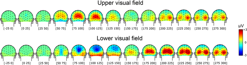
Time course of brain responses to stimuli collapsed across all stimulus conditions in the upper (upper panel) and lower (lower panel) visual field. In both cases, early activity showed maximum amplitude at around 75–125ms, with positive-polarity modulation for upper visual field stimuli and negative-polarity modulation for lower visual field stimuli. Later activity on the other hand showed maximum amplitude around 225–250ms, with positive-polarity modulation in both visual-hemifield conditions.

We then quantified the effects of numerical and non-numerical properties of the dot-array stimuli as well as the visual hemifield manipulation on the ERPs by using a linear mixed-effects model with four factors (numerosity, size, spacing, visual hemifield) as fixed-effects regressors (see Methods; Fig. 3). As shown in Figure 3A, there was a robust effect of numerosity on the ERPs in two latency stages (75–100 ms over Oz and 175–275 ms around bilateral occipital channels), which replicates the previous finding (Park et al., 2016). In particular, the first of the two stages coincided in latency with a very strong effect of the visual hemifield manipulation, reflecting the polarity inversion effect (Fig. 3D). Note that some effects of size and spacing were also observed at different latencies, the point to which we return in the Discussion.

FIGURE 3.

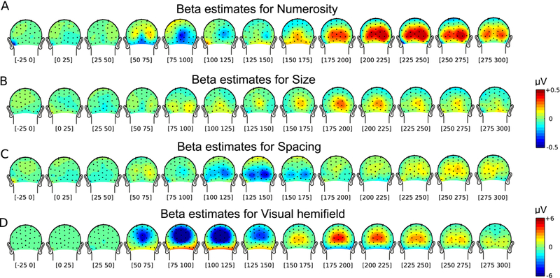
Results of the linear mixed effects model analysis. (A-D) Beta values for the different regressors entered in the analysis as fixed effects, across several time windows. Posterior view of the time course of beta values for numerosity (A), size (B), spacing (C), and visual hemifield (D).

To pinpoint the time point at which the magnitude information is maximally encoded, further preliminary analyses were focused on channels Oz, PO7i, and PO8i, that were previously found to show sensitivity to all magnitude dimensions (Park et al., 2016). In each of these channels, the Euclidean norm of the beta vector comprising the three magnitude dimensions (numerosity, size, and spacing) was plotted to identify the local peaks, as an index of discrete stages of magnitude processing in the visual stream (Fig. 4). At Oz, we looked for peaks in a time window spanning from 0 ms to 150 ms post-stimulus, considering that the effect of visual hemifield (i.e., polarity inversion) is most pronounced in that time frame (see Fig. 3D). As shown in Figure 4A, two noticeable peaks were found at Oz: the first at 55 ms (beta norm = 0.15) and the second at 88 ms (beta norm = 0.41). Later in the time course, the norm of the magnitude beta vector peaked at around 231 ms (norm = 0.59) over PO7i and 213 ms (norm = 0.80) over PO8i (Fig. 4B), largely consistent with the timing found in previous studies (Park et al., 2016; Fornaciai & Park, 2017). These latencies of interest are used in subsequent analyses testing for selective effects of magnitude dimensions (see Section 3.3). Note that while in the regression analysis we first assessed the effect of the three orthogonal dimensions of numerosity, size, and spacing, several other non-numerical visual attributes can be expressed as linear combinations of these dimensions (i.e. individual area, total area, field area, sparsity, coverage, apparent closeness). The effect of these other non-numerical visual cues has been comprehensively assessed in additional analyses (see Section 3.3).

FIGURE 4.

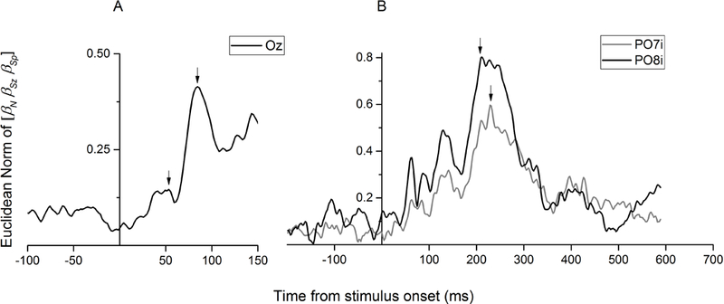
The effects of magnitude (Euclidean norm of the beta vector comprising numerosity, size, and spacing) in the medial occipital (A) and bilateral occipito-parietal (B) channels. The arrows indicate the peak latencies selected for further analysis (55 ms and 88 ms in panel A, 213 ms and 231 ms in panel B).

3.2. Sensitivity to numerosity revealed in the brainwaves.

The degree to which the ERPs were sensitive to various magnitude dimensions was first assessed by plotting brainwaves sorted for different values of numerosity, size, and spacing, separately for upper and lower visual stimulations, as shown in Figure 5. In Oz, brainwaves sorted along different level of numerosity revealed a strong sensitivity to changes in numerosity (Fig. 5A), for both upper and lower visual field stimulations (red and blue waveforms, respectively). The effects of linear contrast waves (weights of [−2 −1 0 1 2]) were tested with a one-sample t-test on the average amplitude of the contrast waves in a 50-ms window around their local peak. The contrast waves for the upper visual-field presentation (orange in Fig. 5D) and for the lower visual-field presentation (cyan in Fig. 5D) were each significantly different from zero (t(29) = 2.45, p = 0.020 and t(29) = −6.60, p < 0.001, respectively for upper and lower visual stimuli). Such sensitivity for changes in numerosity, as reflected by the amplitude of the contrast waves, was stronger than sensitivity to changes along the dimensions of size and spacing, at least for lower visual field stimulation (numerosity versus size, t(29) = −6.17, p < 0.001; numerosity versus spacing, t(29) = −4.26, p < 0.001). On the other hand, the responses to upper visual stimuli (Fig. 5D) showed a weaker sensitivity to numerosity, not significantly different from the sensitivity to either size (t(29) = −0.52, p = 0.60) or spacing (t(29) = 1.13, p = 0.27), the point which we return to in the Discussion (Fig. 5E and 5F).

FIGURE 5.

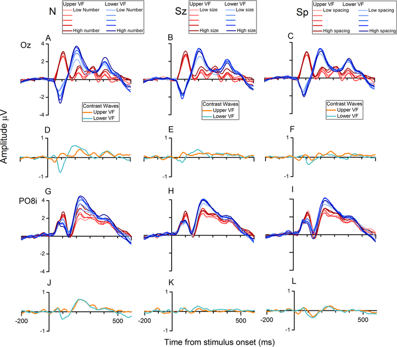
Brainwaves sorted for changes along numerosity, size, and spacing, at channel Oz and PO8i. (A, B and C) ERPs sorted for the different values of numerosity (A), size (B) and spacing (C), for the midline posterior channels Oz. (D, E and F) Contrast waves representing the weighted difference between responses elicited by different levels of numerosity (D), size (E) and spacing (F). Orange waves represent the contrast waves relative to upper visual field stimuli, while cyan waves represent the contrast waves relative to lower visual field stimulation. (G, H and I) Brainwaves sorted along the different values of numerosity (G), size (H) and spacing (I), recorded at the right occipito-parietal channel PO8i. (J, K and L) Contrast waves relative to the different levels of numerosity (J), size (K), and spacing (L) for upper (orange) and lower (cyan) visual field stimulation (channel PO8i).

Regarding the later activity analyzed at PO7i (data not shown) and PO8i, with ERPs peaking at around 230 ms, we first observed that no polarity inversion occurs at these channels, confirming that this phenomenon specifically concerns early-latency ERPs recorded at central occipital scalp locations. Both upper and lower visual stimulation resulted in a strong effect of changes along the dimension of numerosity (PO7i: t(29) = 5.37, p < 0.001 and and t(29) = 5.65, p < 0.001, respectively for upper and lower field stimuli; PO8i: t(29) = 6.85, p < 0.001 and and t(29) = 6.44, p < 0.001, respectively for upper and lower field stimuli), significantly stronger than the modulation provided by either size (PO7i: t(29) =3.29 , p = 0.0026 and t(29) = 3.85, p < 0.001, respectively for upper and lower visual stimuli; PO8i: t(29) = 5.01, p < 0.001 and t(29) = 5.03, p < 0.001, respectively for upper and lower visual stimuli) or spacing (PO7i: t(29) = 2.75, p = 0.0102 and t(29) = 4.89, p < 0.001; PO8i: t(29) = 6.01, p < 0.001 and t(29) = 5.79, p < 0.001). Note that Figure 5 illustrates the brainwaves from PO8i while the data from PO7i is not shown in order to save space; the pattern in PO7i is very similar to that in PO8i and these later-latency effects are not the central focus of this study. Note that while in Fig. 5 we only reported brainwaves sorted along the dimensions of numerosity, size, and spacing, we also assessed the effect of several other non-numerical visual cues. See Section 3.3 for a more comprehensive analysis of the effect of these additional visual attributes.

Interestingly, looking at the brainwaves reported in Fig. 5, brain responses seem somewhat compressed as numerosity increases. According to the relation between stimulus intensity and perception expressed by the Weber-Fechner law, perception should be proportional to the log scaling of intensity, and if this relation holds true also for the corresponding neurophysiological signals, brain responses to log-scaled visual features (number as well as non-numerical attributes) should be largely linear. On the one hand, a possibility is that brain responses might be more compressed compared to the log scaling of the perceptual representation of numerosity. Future studies should investigate the nature of this difference between the pattern of compression observed at the behavioral and neural levels.

3.3. Testing for selective sensitivity to magnitude dimensions

Finally, we examined the degree to which ERPs, at distinctive processing stages, were uniquely modulated by various quantity dimensions. To do so, we computed the angle between various magnitude dimensions and the parameter estimate vector β computed from the earlier (Oz) and later (PO7i/PO8i) time points. Such a measure allowed us to assess which one of these candidate dimensions best contributes to the modulation of the ERPs in those stages. Figure 6 and Figure 7 show the results of this “angle analysis” by graphically demonstrating the angle between β and all the other candidate dimensions calculated over a 20-ms (Oz) or 50-ms (PO7i and PO8i) time window around the latencies selected in the preliminary analysis. Note that different window sizes were used to better capture the effect at different latencies. Indeed, while early responses tend to have a fairly narrow peak of activity, later responses are typically better captured by a broader time window.

FIGURE 6.

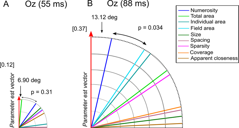
Angle analysis at early latency stages of magnitude processing. We assessed which one of the candidate dimensions best represents the beta estimates vector at the channels and latencies identified with the ROI selection and regression analyses, in the C1 range. Angle between the parameter estimate vector and all the candidate dimensions (A) for channel Oz at 55 ms, (B) for channel Oz at 88 ms. Values inside square brackets represent the Euclidean norm of the parameter estimate vector. The size of each polar plot is scaled according the norm of the parameter estimate vector.

FIGURE 7.

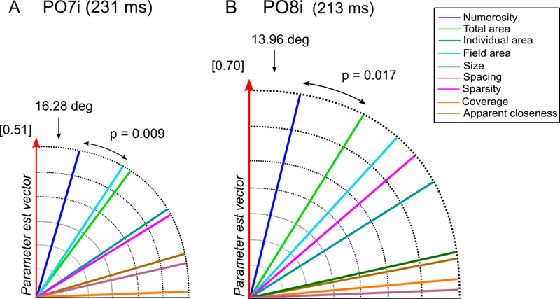
Angle analysis over the bilateral occipital channels in the P2p latency range. Angle between the parameter estimate vector and all the candidate dimensions (A) for channel PO7i at 231 ms, (B) for channel PO8i at 213 ms. Values inside square brackets represent the Euclidean norm of the parameter estimate vector. The size of each polar plot is scaled according the norm of the parameter estimate vector.

In extremely early (55 ms) responses at Oz, there was no clear winner: while total area was the dimension lying closest to the beta vector followed by numerosity (Fig. 6A), the difference between the two angles did not reach statistical significance (p = 0.31). This result suggests that at this time point brain responses are not specifically sensitive to any particular dimension. Furthermore, it should be noted that substantially smaller Euclidean norm of β (0.12, compared to 0.37–0.70 in other sites/latencies) suggests that the ERPs at Oz around 55 ms do not contain much information about the quantity manipulation overall. For the later peak (88 ms; Fig. 6B) at Oz, numerosity resulted as being the dimension closest to the parameter estimate vector (angle = 13.12 deg), followed by field area (angle = 34.66 deg). Moreover, the angles of the two dimensions resulted to be significantly different (p = 0.034), demonstrating that signals at around 88 ms are specifically sensitive to the numerosity dimension.

Regarding the later activity recorded at PO7i (231 ms) and PO8i (213 ms), we observed a very strong sensitivity for numerical information (Fig. 7A and 7B), as shown by numerosity resulting in both cases the dimension closest to β, with an angle significantly smaller compared to the second closest dimension (PO7i: 16.28 deg versus 33.39 deg, respectively for numerosity and total area; p = 0.009; PO8i: 13.96 deg versus 31.73 deg, respectively for numerosity and total area; p = 0.017). This result again shows that at this later time point brain signals are highly sensitive to numerosity, more than to any other non-numerical dimension.

4. Discussion

Despite the growing amount of studies dedicated to uncovering the mechanisms of numerosity perception, the precise time course of the underlying processing, and the neural loci are still unclear. ERP studies (e.g. Temple & Posner, 1998; Libertus et al., 2007) have suggested that the main stage of numerosity processing takes place at around 150–200 ms from the stimulus presentation. Moreover, neuroimaging studies of numerosity processing have provided strong evidence for the role of the intraparietal sulcus (IPS) in the analysis of numerical information (i.e. Piazza et al., 2007; Harvey et al., 2013; Castaldi et al., 2016). Nevertheless, recent ERP studies from our group suggest that IPS might not be the very first level of numerosity processing (Park et al., 2016; Fornaciai & Park, 2017), supporting the hierarchy of processing stages proposed by Dehaene & Changeaux (1993) in their influential computational model of numerosity perception (see also Verguts & Fias, 2004, for a similar model including also symbolic numerosity). According to Dehaene & Changeaux’s (1993) model, raw numerosity information must be first converted into a size-invariant and shape-invariant code, before being transmitted to a subsequent number-sensitive summation or accumulation stage, and finally to a number-selective stage. So, the first level of numerosity processing would be a normalization stage, where the items are encoded in an object-location map irrespective of their features, in order to limit influences from other continuous magnitudes.

Evidence for an initial processing stage for numerosity information was hinted by Park and colleagues (2016), showing very early sensitivity to numerosity (~ 75 ms) peaking at midline occipital scalp sites, followed by later sensitivity (~ 180 ms) over occipito-parietal scalp sites in response to visual dot arrays. Neural activity from both of these latency windows was specifically sensitive to modulations in the number of items presented, and more sensitive to numerosity than any other non-numerical attribute (size and spacing). Park and colleagues posited that while the later activity may reflect an accumulation stage, showing sensitivity to numerosity in the P2p latency range, early selectivity to numerosity may reflect the first stage of image normalization proposed by Dehaene & Changeaux’s (1993) model. However, while other previous studies provided strong evidence for the localization of the second stage proposed by Dehaene & Changeaux (1993) in the parietal cortex – and particularly in IPS, where neuronal populations potentially show tuning functions for numerosity (Piazza et al., 2007; Harvey et al., 2013) – little is known about the earlier stages of numerosity processing.

In the present study, we tested whether the early selectivity for numerosity initially discovered in Park et al. (2016) arises from early visual areas – such as V1, V2 and V3 – or from later visual areas along the dorsal stream. Indeed, according to the idea of number as a primary perceptual feature (Burr & Ross, 2008; Fornaciai et al., 2016; Anobile et al., 2016), it seems likely that the processing stream subserving numerosity perception might start very early in the visual hierarchy. However, while the results of Park and colleagues (2016) provide clear evidence about the timing of the first stage of numerosity-sensitive activity, no more specific conclusion could be drawn from timing information alone, and the poor spatial resolution of EEG scalp recording could not be used to precisely localize the source of early activity.

To shed light on the possible localization of the early stages of numerosity processing, we capitalized on the results from numerous previous studies showing a peculiar pattern of ERP polarity inversion for signals arising from early visual areas, when the stimuli are presented either in the upper or lower visual hemifields (Clark et al., 1995; Di Russo et al., 2002). This inversion of polarity resulting from stimulation of the upper or lower visual field – evident in the latency range of the C1 component – has been attributed to the peculiar folding pattern of V1 and other early visual areas around the calcarine sulcus in the occipital cortex (Clark et al., 1995), predicted by the “cruciform model” of the primary visual cortex (Jeffreys & Axford, 1972a).

The possibility to precisely isolate signals arising predominantly from V1 using upper and lower visual field stimulation, however, has recently been debated across a series of empirical and simulation studies (i.e. Ales et al., 2010; Ales et al., 2013; Kelly et al., 2013a; Kelly et al., 2013b). According to the “cruciform” model of early visual areas (Jeffreys & Axford, 1972a; 1972b), not only will V1 give rise to opposite polarity responses, but V2 and V3 may also give contributions, and very careful stimulation is needed to successfully segregate contributions of striate and extrastriate areas (i.e. requiring relatively small stimuli and optimal locations in the upper and lower visual field) (Di Russo et al., 2002; Kelly et al., 2013a). However, as a general rule to distinguish V1 polarity signature from other areas, the cruciform model provides a clear prediction. According to Kelly et al. (2013a), given the unique anatomical features of V1 and the localization of V2 and V3, the inversion of polarity predicted for V1 and that predicted for V2/V3 should be in opposite directions – an idea based on the dipoles describing neural generators of scalp signals located in the striate or extrastriate cortices. Specifically, according to this idea, activity generated in V1 should be reflected by a surface-negative pattern of activity, consisting in negative- and positive-polarity VEPs respectively for the upper and lower visual hemifields. On the other hand, signals generated in V2/V3 should show surface-positive activation, resulting in positive-polarity scalp potentials for upper visual field stimuli, and negative-polarity potentials for those in the lower visual field (Ales et al., 2013; Kelly et al., 2013a; Kelly et al., 2013b). So, while the use of EEG recording in previous work (Park et al., 2016) limits the conclusions based on scalp topography, exploiting the polarity inversion effect provides a clear way to pinpoint a more specific candidate brain area as the substrate of early numerosity processing.

Our results showed a strong pattern of polarity inversion in the early portion of neural responses to stimuli presented in the upper versus lower visual hemifields, specifically for signals recorded over midline occipital scalp sites (Oz) (see Fig. 3D and 5A–5C). This result is consistent with the view that these VEPs recorded over midline occipital scalp sites arise from neural generators located in early visual areas. In contrast, no inversion of polarity was observed in the ERPs recorded over more lateral, occipito-parietal channels (PO8i).

More specifically, the early responses recorded at channel Oz around 50 ms (reflected by the peak of the magnitude β norm at 55 ms) showed signs of surface-negative activation (see Fig. 5D), with upper visual field stimuli resulting in negative-polarity activity and lower visual field stimuli resulting in positive-polarity ERPs, which suggests activity generated in V1. On the other hand, later on in the time course, at around 90 ms (reflected by the peak of the magnitude β norm at 88 ms), we observed a clear surface-positive pattern of activation, resulting in positive ERPs when the stimuli were showed in the upper visual field, and negative ERPs when the stimuli were presented in the lower visual field (see Fig. 5D). This surface-positive pattern suggests a stronger contribution of area V2 and V3 in such signals. The important point is that, while the first (55 ms) of the two peaks did not show signs of sensitivity to any magnitude dimension, ERPs from the second peak (88 ms) showed selective sensitivity to numerosity, suggesting that the neural activity at this stage can be most parsimoniously explained by the modulation of numerosity. One interpretation of these results concerns the possibility of two processing stages in the visual stream, the first based on V1 and the second on V2/V3 regions. According to this view, while V1 might be not particularly selective to any of the magnitude dimensions, the second stage based on V2/V3 is strongly sensitive to numerical information. However, since activity at the earlier peak (55 ms) was much weaker compared to later activity (88 ms), further work will be needed to demonstrate whether that earlier activity is driven solely by V1.

Indeed, it is important to note that interpreting the source of such signals requires caution (Clark et al., 1995; Di Russo et al., 2002; Kelly et al., 2013a). In particular, using relatively large stimuli likely causes a spread of activity across different networks that might mask specific contributions from single areas. Clark et al. (1995) showed that the pattern of polarity inversion of signals originating in V1 has a distinct topography, with an asymmetric reversal point located between −21 and −35 deg under the horizontal meridian, and that accurate mapping of specific contributions from V1 requires small and carefully placed stimuli. So, due to the relatively large stimuli used in our paradigm (which was inevitable in the context of our research question) it is not possible to entirely rule out V1 contributions to the VEPs. Rather, the peak found at 88 ms might reflect activity from both V1 and V2/V3, with a more prominent surface-positive contribution from these latter two areas. Note, however, that regardless of whether or not V1 is involved in numerosity processing, the current results do indicate that numerosity processing starts at the latest at the level of V2 and V3.

Previous attempts to localize the different stages of numerosity processing, mostly carried out by exploiting fMRI techniques, have provided mixed results. With the exception of Roggeman and colleagues (2011), who found fMRI responses in the inferior occipital gyrus, no other study has described number-sensitive activation in early visual cortices (e.g. Piazza et al., 2007; Harvey & Dumoulin, 2017). Such seemingly inconsistent results may be best explained by differences in the stimuli, experimental paradigms, and recording techniques. More specifically, most previous studies used very small numerosities (i.e. 1–7) or very different techniques aiming to find evidence for number-selective activation patterns (e.g., fMRI adaptation and population receptive field modeling). Particularly, in the case of very small numerosities, previous investigations (Fornaciai & Park, 2017) showed that number-sensitive activity at early latencies is nearly absent when the stimuli were in the subitizing range (i.e. 1–4). These results have been linked to the specific nature of the brain mechanisms dedicated to the processing of such small numerosities (i.e. attentional object individuation), which appears to be different from the mechanisms supporting the processing of larger numerosities. Interestingly, looking at the results provided by Roggeman et al. (2011), the activation related to the location coding in the inferior occipital gyrus seems like it may partially extend to early visual areas, and possibly to areas V2 and V3. So, although the authors did not report a more refined localization of the activity, these results would be consistent with our findings. However, due to the fine temporal resolution of EEG recording, our paradigm additionally provides evidence that number-sensitive activation in early visual areas reflects the initial feed-forward sensory activity, and not later feedback signals – an information that could not be gained by using other techniques such as fMRI.

On the other hand, is it possible that such extremely early activity found in our study might have been driven by differences in other low-level parameters of the stimuli, such as overall luminance and global contrast? Our analyses showed that this is not the case, since global luminance and contrast are dimensions tightly linked to the overall area occupied by the dots and our results clearly showed that total item area did not provide a meaningful modulation of the brain responses.

Overall, current results suggest early stations of visual processing are selectively sensitive to numerosity information of a dot array. Nevertheless, some signs of an influence from non-numerical dimensions seem apparent also later on in the brain responses (Fig. 3B and 3C), while previous results showed very little influence of magnitudes different from numerosity (Park et al., 2016). This observation is however not surprising, and can be explained considering the difference in the visual stimulation parameters used in the two studies, and particularly by the eccentricity of the stimuli. While Park and colleagues (2016), used central stimuli, here we adopted relatively peripheral stimuli in order to differentiate the responses to upper and lower visual stimulation. Even with a relatively small eccentricity from the fovea (3.75 deg), exploiting such peripheral stimuli might have hampered object segmentation processes, promoting a more pronounced influence from non-numerical dimensions.

Indeed, previous behavioral studies (Anobile et al., 2015) have demonstrated that eccentricity plays an important role in the switching from numerosity to a texture-density regime, with both regimes defined on the behavioral level by the rate of changes in precision as the numerosity increases (linearly or with the square-root of numerosity, respectively; Anobile et al., 2014). In short, the transition between the two regimes depends not only on the density of the items, but also on the eccentricity of the stimulus, with a lower critical density (i.e. the density threshold determining the switch between numerosity and texture-density regimes) as the eccentricity increases –resembling the Bouma law governing crowding effects (Bouma, 1970; Levi, 2008; Pelli & Tillman, 2008; Anobile et al., 2015).

The results of Anobile and colleagues’ (2015) study showed that while with central stimuli the critical density is about 2 dot/deg², moving the stimuli to an eccentricity of 5 deg caused the value to drop to about 0.95 dot/deg². In the current work, the (center-to-center) eccentricity of the stimuli was set to 3.75 deg, while the density of the stimuli ranged from 0.18 to 2.91 dot/deg², according to the different combinations of numerosity and field area. Given these parameters, a small portion of our stimuli might have triggered a texture-density regime, making the effects of non-numerical magnitudes to emerge in brain signals. Moreover, the weaker sensitivity for numerosity found for responses to upper visual field stimuli, especially at early latency (Fig. 5A), is not surprising as well. Indeed, it is well known that while right and left visual hemifields are represented in a largely symmetric way, marked differences exist for the upper and lower hemifields, reflecting a generalized “lower field advantage”, evident both at the behavioral level (i.e. faster reaction times, higher resolution and greater sensitivity; He et al., 1996; Danckert & Goodale, 2001; Talgar & Carrasco, 2002; Levine & McAnany, 2005) and at the neurophysiological level (i.e. shorter latencies and higher amplitude of VEPs; Lehmann & Skrandies, 1979; Fioretto et al., 1995; Kremláček et al., 2004; Hagler, 2014). Thus, it is likely that the increased effect of non-numerical dimensions due to the eccentricity of the stimuli has been enhanced in the upper compared to lower visual field due to such asymmetries. However, these observations do not hamper our conclusions about the role of early visual areas in numerosity processing, and the overall pattern of sensitivity to numerosity found at most of the target latencies demonstrates that brain signals were nevertheless much more sensitive to changes in numerosity than to any other dimension. This is not to say that size, spacing, or other non-numerical visual attributes are not encoded in early visual areas, but that modulation of numerosity processing best explains the pattern of neural activity elicited by dot arrays that varies systematically in a variety of magnitude dimensions.

Regarding the activity in the P2p latency range observed at both PO7i and PO8i, our findings successfully replicate previous results (i.e. Temple & Posner; Libertus et al., 2007; Hyde & Spelke, 2009; Park et al., 2016; Fornaciai & Park, 2017) showing strong selectivity for numerosity at later processing stages, namely in the latency range of the P2p component. More specifically, we found that brainwaves over occipito-parietal scalp locations show a strong sensitivity to changes in numerosity (Fig. 5) in a broad latency window around 200–250 ms after stimulus onset (i.e. consistent with the timing of the P2p component observed in previous studies; Temple & Posner, 1998; Libertus et al., 2007). Besides the modulation found in the brainwaves analysis, further analyses confirmed that such responses are indeed mainly modulated by numerosity, with little contributions from other non-numerical visual attributes (Fig. 7). These later number-sensitive responses are commonly associated with approximate numerical processing of moderate numerosities (>4 items), and could potentially reflect a summation-coding mechanism likely residing in the parietal cortex. Moreover, the results at the level of the P2p component confirm that the polarity inversion is specifically occurring only in the earlier portion of the evoked potentials recorded at central occipital channels, and that it is not a generalized phenomenon or a by-product of our stimulation paradigm, thus strengthening the conclusion that early signals around the C1 latency window actually reflect the initial feed-forward activity in early visual areas.

5. Conclusion

In sum, the polarity inversion of the ERPs in response to dot arrays presented in the upper and lower visual fields indicates that early visual areas are involved in numerosity perception. The polarity-inversion paradigm requires increased eccentricity of the dot-array stimuli, which have resulted in more pronounced contribution of non-numerical visual attributes on neural responses, unlike previous studies with central vision stimulation (Park et al., 2016). Despite this difference, the present results demonstrate that very early signals are consistently sensitive to numerosity and provide evidence that numerosity processing starts very early (at least in V2/V3) in the cortical visual hierarchy.

FIGURE 1.

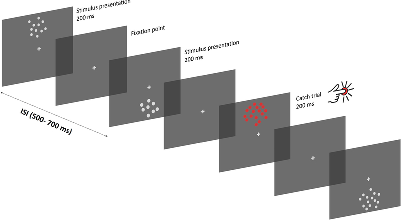
Procedure. Participants were asked to fixate on the central fixation cross while stimuli were displayed on the screen for 200 ms, either in the upper or lower portion of the screen (center-to-center eccentricity = 3.75 deg). Different stimuli were divided by blank periods where only the fixation point was displayed, with a variable ISI of 500–700 ms between successive presentations. Occasionally, a red dot-array was showed, and in such cases participants were instructed to press a button on a joypad as soon as possible.