Solvation dynamics: Improved reproduction of the time-dependent Stokes shift with polarizable empirical force field chromophore models

Abstract

The inclusion of explicit polarization in molecular dynamics simulation has gained increasing interest during the last several years. An understudied area is the role of polarizability in computer simulations of solvation dynamics around chromophores, particularly for the large solutes used in experimental studies. In this work, we present fully polarizable ground and excited state force fields for the common fluorophores N-methyl-6-oxyquinolium betaine and Coumarin 153. While analyzing the solvation responses in water, methanol, and the highly viscous ionic liquid 1-ethyl-3-methylimidazolium trifluoromethanesulfonate we found that the inclusion of solute polarizability considerably increases the agreement of the obtained Stokes shift relaxation functions with experimental data. Solute polarizability slows down the inertial solvation response in the femtosecond time regime and enables the chromophore to adapt its dipole moment to the environment. Furthermore, the developed chromophore force field reproduces the solute dipole moments in both the electronic ground and excited state in environments ranging from gas phase to highly polar media correctly. Based on these studies it is anticipated that polarizable models of chromophores will lead to an improved understanding of the relationship of their environment to their spectroscopic properties.

1. Introduction

The investigation of solvent properties via calculation or measurement of the time-dependent Stokes shift (TDSS) has been of high interest during the last decades.^1–20 The TDSS probes the timescale of solvent rearrangement by excitation of a dissolved chromophore, which causes the solvent to reorganize and the wavelength of the emitted fluorescence light of the chromophore to change. Upon excitation, both the dipole moment and the polarizability of the chromophore change, so that both the electrostatic and dispersion interactions change.²¹ In recent years, the increasing accuracy and resolution of experiments facilitated the detailed analysis of even very small effects on the TDSS, such as the probe dependence of the obtained timescale,^14,22 or the change in the TDSS upon addition of a side chain to a chromophore.²³ To account for such small effects in computer simulation more accurate solvent and chromophore models are needed. Recently, we showed that it is possible to considerably increase the agreement of computational TDSS to experiment by the use of polarizable solvent models in molecular dynamics simulation of polar solvents and ionic liquids.^24–27 However, the chromophore models remained nonpolarizable due to difficulties of describing polarizability in the excited state in a consistent fashion.

In fact, polarizable computer simulations of the TDSS to date comprise only artificial mono- or diatomic probe molecules,^28–30 theoretical models,^31,32 or combined approaches where the chromophore is treated quantum-mechanically or semi-empirically.^19,20,33,34 Stratt and coworkers³⁵ recently used a polarizable model of Coumarin 153 to calculate solute-pump/solvent probe spectra, where the polarizabilities of each atom were obtained by regression of the molecular quantum-mechanical value. Although the mentioned studies confirm that solute polarizability has profound impacts on the TDSS, namely slowing down the observed response and broadening the distribution of the energy gap, the computational TDSS of polarizable, experimentally-relevant chromophores has yet to be carefully studied.

We therefore developed polarizable models of two commonly used fluorophores, N-methyl-oxyquinolinium betaine (MQ) and Coumarin 153 (C153) and computed the TDSS in two polar solvents and one ionic liquid. Since the inclusion of polarizability enables a molecule to react to changes in environment, we chose water, methanol, and 1-ethyl-3-methylimidazolium trifluoromethanesulfonate as solvents to cover a wide range of polarities. The use of an ionic liquid furthermore allows us to monitor the behavior of the newly created force field in a highly charged environment, where Coulombic forces dominate.

The present study both confirms that prior research on the influence of solute polarizability on solvation dynamics is also applicable for large chromophores, as well as provides a detailed analysis of the effects of polarizability of experimentally-relevant solutes. Furthermore, the agreement of the computational TDSS to experiment is raised considerably by the use of polarizable solute force fields.

The remainder of this article is organized as follows. In section 2 the setup of the polarizable force field for MQ and C153 is discussed and details on the simulation of the TDSS are given. A detailed analysis of the influence of solute polarizability on the observed TDSS response functions, as well as on the solute dipole moment distributions and solvent structure is given in section 3. Concluding remarks are presented in section 4.

2. Methods

This study deals with the two chromophores N-methyl-6-oxyquinolinium betaine (MQ) and Coumarin 153 (C153), depicted in Fig. 1. C153 is a commonly used fluorophore, which increases its dipole moment upon excitation.^{2,14,22,34–38} In contrast, MQ lowers its dipole moment upon excitation, which makes it an interesting test case, and has gained increasing interest due to its small size and rigid structure.^{14,19,20,39–41} As solvents, methanol (MeOH) and the ionic liquid 1-ethyl-3-methylimidazolium trifluoromethanesulfonate (EmimOTf) were chosen. Water was also examined, but only with MQ since C153 is not soluble in water.

Fig. 1.

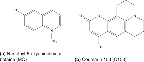
Chromophores used in this study.

2.1. Chromophore force field

A polarizable chromophore force field was generated as follows. Initial parameters for the polarizable force field describing MQ and C153 were taken from the previously used nonpolarizable models described in Ref. 24 and Ref. 27 which relied on bonded parameters obtained from PARAMCHEM^42,43 and the CHARMM General Force Field (CGenFF).⁴⁴ The partial charges from Ref. 24,27 which were obtained from quantum-mechanical (QM) calculations (density function theory (DFT) or time-dependent DFT (TD-DFT) with the ωB97×D hybrid DFT functional⁴⁵, an aug-cc-PVTZ basis set, the CHelpG method⁴⁶ and polarizable continuum model (PCM) of water) were also reused, but scaled. Since the partial charges in the nonpolarizable model were chosen to over-estimate the gas phase dipole to account for polar environments, the charges were scaled by 0.88 (MQ) or 0.90 (C153) which recovered gas phase dipoles well. In a polarizable model, a change of dipole moment with environment is realized solely via the inclusion of polarizability. Scaled PCM charges were used instead of unscaled gas phase charges, since the partial charge changes of MQ upon excitation were shown to be physically implausible in the case of gas phase QM calculations. ⁴⁷ The atomic polarizabilities were obtained quantum-mechanically as described in Ref. 47,48 on geometries optimized at a MP2/6–31G(d) model chemistry. All QM calculations were carried out with Gaussian09⁴⁹ and Psi4.^50,51 Polarizabilities in the ground state of MQ and C153 were calculated on the RI-MP2 level of theory with Sadlej’s polarizable PVTZ basis set. ⁵² Excited state polarizabilities were obtained by scaling each of the ground state atomic values by the factors published in Ref. 47. Both ground and excited state polarizabilities were scaled uniformly by a factor of 0.724, as suggested for aromatic compounds.⁵³ Thole screening factors were chosen to match those in similar structures in the CHARMM Drude force field (see Ref. 53,54 and references therein) and slightly adjusted to recover the molecular polarizabilities and their components in the x, y and z-direction well. For MQ, a ground-state polarizability of 16.2ų was obtained (unscaled 22.3 ų), which agrees sufficiently well with results from Ernsting and coworkers,⁹ who reported a value of 20.0ų. Upon excitation, the polarizability increases to 17.2ų. For C153 a polarizability of 23.2ų was obtained for the ground state and 24.5 ų for the excited state. The atom types in MQ and C153 were changed to the appropriate types in the CHARMM Drude force field, and parameters updated according to the bond, angle, dihedral, and Lennard-Jones parameters present in the Drude force field. For MQ, the remaining angle and dihedral parameters were optimized to recover QM dihedral scans and vibrational spectra at the MP2/6–31G(d) model chemistry according to the protocol published in Ref. 53. For C153, the remaining angle and dihedral parameters were reused from Ref. 27. The force fields are available in the ESI^†.

2.2. Simulation setup

For each system, 500 to 1000 starting replicas were obtained from the equilibrated simulations of nonpolarizable chromophores in Ref. 24,27, re-equilibrated with the polarizable chromophore, and then excited by replacing the ground state force field by the excited state force field (change of partial charges and polarizabilities). Then, the trajectories were monitored until the surrounding solvent completely relaxed to the new state. The respective number of replicas, as well as equilibration and production periods are given in Table 1. Additionally one very long simulation in the ground and excited state of MQ and C153 in each of the solvents was conducted, to analyze the solvent structure and energy gap distribution in equilibrium. The length of the equilibrium trajectories was at least 10 ns in water and methanol, and at least 70 ns in the ionic liquid.

Table 1.

Simulation setup, number of independent replicas, equilibration periods, production periods and temperature

System	# Reps	Equil.	Prod.	Temp.
1 MQ + 1000 H2O	1000	50ps	50 ps	293 K
1 MQ + 1000 MeOH	1000	100 ps	100 ps	300 K
1 C153 + 1000 MeOH	500	100 ps	100 ps	300 K
1 MQ + 500 EmimOTf	500	250 ps	2500 ps	300 K
1 C153 + 500 EmimOTf	500	250 ps	2500 ps	300 K

All simulations were carried out with the program package CHARMM.⁵⁵ We used the SWM4-NDP water model,⁵⁶ the MeOH model from Ref. 57 and the polarizable EmimOTf model described in Ref. 27 with force field parameters from Padua and coworkers,^58–60 and polarizabilities from Ref. 61. All calculations made use of the Velocity-Verlet integrator with a time step of 0.5 fs and a dual Nosé-Hoover thermostat.^62,63 Periodic boundary conditions were applied. Electrostatic interactions were calculated employing the particle Mesh Ewald method with a grid size of approximately 1 Å, cubic splines of order 6, and an Ewald parameter of κ = 0.41Å⁻¹. Van der Waals interactions were cut off at 12Å, using a smooth switching function between 10 and 12Å. The SHAKE algorithm⁶⁴ was applied to keep bonds to hydrogens at a fixed length, and Drude particles were restricted to a maximum distance of 0.2Å. The Drude particles of MQ and C153 were assigned a mass of 0.2 amu. Additional simulations featuring Drude masses of 0.4 amu are presented in the ESI of this article.^† The trajectories were analyzed via a self-written python program, which makes use of the MDAnalysis program package, ⁶⁵ and the time-dependent Stokes shift calculated as the change in electrostatic interaction energy ΔU(t) of the chromophore to the surrounding solvent between ground and excited state. 95% confidence intervals were calculated as $\overline{\mathrm{\Delta }U}\pm \frac{t\cdot s}{\sqrt{n}}$ where t is the Student t factor, s the standard deviation and n the number of trajectories.

3. Results and discussion

3.1. Dipole moments

The dipole moment of the chromophore and its change upon excitation resembles the most important electrostatic property of the probe responsible for solvation dynamics. Table 2 lists the dipole moments of MQ and C153 in different environments obtained from MD simulations. The inclusion of the polarizability of the dye enlarges the dipole moment in polar environments, and correctly recovers gas phase values. In literature, the ground and excited state dipole moments for MQ are 10.1–11.0D and 5.8–7.2D in the gas phase^24,39,40,47 and 15.3–22.0D and 8.6–14.0D in water, respectively. ^19,24,47 The obtained MQ dipole moments in this study thus agree well with literature. For C153, values of 5.6–7.0D and 11.8–14.0 D are documented in the literature for the electronic ground and excited states in the gas phase, respectively.^34,47,66 In MeOH dipole moments of 9.9 D and 18.7 D are reported, respectively. ⁴⁷ All reported data is in good agreement with the dipole moments reported in this study, although the gas phase dipole moment is slightly overestimated. Thus, our polarizable models of MQ and C153 are able to reproduce the correct dipole moments in different environments for both the electronic ground and excited state.

Table 2.

Dipole moments of MQ and C153 obtained from molecular dynamics simulation with polarizable (pol. FF) and nonpolarizable (nonpol. FF) chromophore force fields in different environments. All solvent force fields were polarizable All values in Debye.

		MQ		C153
	environment	${\mathbb{S}}_0$	${\mathbb{S}}_1$	${\mathbb{S}}_0$	${\mathbb{S}}_1$
Pol. FF:	H2O	19.0	12.4	-	-
	MeOH	17.4	10.4	10.4	17.6
	EmimOTf	15.5	9.4	10.1	17.2
	in vacuo	11.0	7.1	8.4	13.9
Nonpol. FF:	all media	16.4	10.0	10.9	18.9

Fig. 2 depicts the distribution of dipole moments of MQ and C153 in different solvents obtained from equilibrium simulations. Whereas the nonpolarizable models cannot react to changes in the environment (dashed lines), the polarizable models show a broad distribution centered around the values given in Table 2. The absolute dipole moments, as well as the change in dipole moment upon excitation depend strongly on the solvent in the case of MQ, but not for C153. This finding agrees well with literature, where the change in dipole moment of C153 was found to be largely invariant to the respective solvent.^34,66,67

Fig. 2.

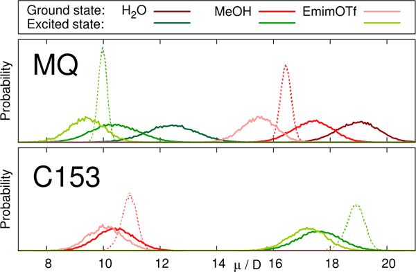
Distribution of dipole moments of MQ (top) and C153 (bottom) in the ground (red) and excited (green) state in different solvents.

Continuous lines represent the polarizable chromophore models, dotted lines represent the nonpolarizable models.

3.2. Time-dependent Stokes shift

The time-dependent Stokes shift of a chromophore in solution is a measure of solvation dynamics. Fig. 3 depicts the absolute and relative (inset) Stokes shift relaxation function of MQ in water. The light green line corresponds to the simulation employing a nonpolarizable chromophore and polarizable water model from Ref. 24, where the inertial subpicosecond response is too fast compared to experiment. The use of the polarizable solute force field (dark green line) slows down the inertial response considerably, thus leading to a much better agreement with experiment. Since water relaxation is very fast, the exact measurement of the Stokes shift is comparably challenging, and the deviations between different measurements are quite substantial. Thus, two experimental datasets are given in Fig. 3 in dark²³ and light red.³⁹ The diffusive relaxation at longer timescales, as depicted in the inset of the figure, is not affected by the solute model. Therefore, both the nonpolarizable and the polarizable chromophore model depict the normalized experimental Stokes shift well after 0.1 ps. Since C153 is not soluble in water, no simulations of C153 in water were conducted.

Fig. 3.

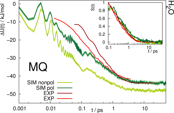
Absolute Stokes shift of MQ in water. Experimental data from Ref. 23 (dark red) and 39 (light red). The colored area corresponds to a 95% confidence interval. Inset: Relative Stokes shift, normalized at 0.1 ps.

A similar picture arises for the Stokes shift of MQ and C153 in methanol, shown in Fig. 4. The too fast inertial response for nonpolarizable chromophore models is slowed down by inclusion of polarizability, thus leading to a better agreement with experiment. It should be noted that within experiment, the wavelength at t = 0 can only be extrapolated. Thus the absolute shift comes with a considerable amount of uncertainty and experimental studies disagree on the magnitude. This effect is especially pronounced for C153 in methanol, where for example Ref. 14 reports an overall shift of 36.7kJ/mol, whereas much lower values (28.0 to 30.0kJ/mol) were reported in earlier studies.^29,36 Thus, the experimental Stokes shift from Ref. 14 was scaled to 28.0kJ/mol and is depicted as dashed line in Fig. 4. Regardless of the magnitude of the overall shift, the curvature and timescales of the inertial relaxation are better described by the polarizable models, although there is still some disagreement to experiment.

Fig. 4.

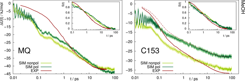
Absolute Stokes shift of MQ and C153 in methanol. Experimental data from Ref. 14 (dark red). The dashed line corresponds to the experimental values with different absolute shift (28.0 kJ=mol instead of 36.7 kJ=mol). The colored area corresponds to a 95% confidence interval. Inset: Relative Stokes shift, normalized at 0.1 ps.

Since solvation dynamics on femtosecond timescales are difficult to measure, and the resolution usually corresponds to dozens or hundreds of femtoseconds, the agreement of the polarizable simulations with experiment is still satisfying.

Fig. 5 depicts the absolute Stokes shift of MQ and C153 in the ionic liquid EmimOTf. For MQ, no experimental data is available, since the ground state MQ is protonated in EmimOTf due to the high acidity of the C₂-hydrogen of the imidazolium cation, whereas the proton is lost in the excited state via proton transfer,⁶⁸ which renders a direct measurement of the TDSS impossible. For C153 the polarizable simulations (dark green) agree much better with experiment (red line) than the nonpolarizable simulations (nonpolarizable solvent and solute, yellow line) from Ref. 69 or the half-polarizable simulations (polarizable solvent but nonpolarizable solute, light green) from Ref. 27. Interestingly, the combination of polarizable solvent but nonpolarizable solute leads to the largest disagreement with experiment in the initial time regime, where the solvent polarizability enables a quick relaxation which is not counteracted by solute polarizability.

Fig. 5.

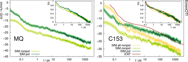
Absolute Stokes shift of MQ and C153 in the ionic liquid EmimOTf. Yellow: Simulation with nonpolarizable solute and solvent. Experimental data from Ref. 70 (dark red). The colored area corresponds to a 95% confidence interval. Inset: Relative Stokes shift, normalized at 0.1 ps.

Table 3 lists the integral relaxation times (τ) of all systems, which were obtained via fitting of the absolute Stokes shift response function to the triexponential function

$$f(t)=a_0+\sum _{i=1}^3{a}_i\cdot e^{-\frac{t}{{\tau }_i}}$$ (1)

as

$$\langle \tau \rangle =\frac{{\sum }_{i=1}^3{a}_i{\tau }_i}{{\sum }_{i=1}^3{a}_i}.$$ (2)

Table 3.

Relaxation times (τ) of the TDSS obtained from simulations with nonpolarizable solvent and chromophore (np/np), polarizable solvent and nonpolarizable chromophore (p/np) and polarizable solvent and chromophore force fields (p/p)

		Simulation			Experimenta
		np/np	p/np	p/p
MQ	H2O	-	0.29 ps	0.45 ps	0.57 ps23, 0.48 ps14
	MeOH	-	2.99 ps	3.37 ps	2.69 ps14
	EmimOTf	-	0.15 ns	0.24 ns	-
C153	MeOH	-	3.03 ps	3.34ps	3.04 ps14
	EmimOTf	0.23 ns	0.25 ns	0.28 ns	0.61ns70 (0.26 nsb)

^aExperimental (τ) as given in the respective references, where relaxation times were obtained in parts usign different fitting algorithms and extrapolated t = 0.

^bThe experimental relaxation time of C153 in EmimOTf is 0.26 ns when integrated up to 2.5 ns (the length of the trajectories in this study).

The respective fit parameters are given in the ESI.^† The relaxation times are affected slightly by the use of a polarizable chromophore force field. As visible from the insets in Fig. 3, 4 and 5, the diffusive timescales of the TDSS are nearly not affected by addition of chromophore polarizability. The observed changes in relaxation times thus stem from the slower inertial relaxation, which shifts the TDSS upwards compared to the nonpolarizable chromophore force field, thus producing longer integral relaxation times. The obtained TDSS timescales, which mainly reflect the behavior of the solvent, and thus the quality of the solvent force field, agree sufficiently well with experiment for both the polarizable and nonpolarizable chromophore force fields.

Within all investigated solvents, the relaxation in the first few femtoseconds is too large when employing polarizable solvent models together with nonpolarizable chromophore models. The excitation of the chromophore creates a large electric perturbation, to which the solvent electronic degrees of freedom react immediately. However, the unfavorable conformation of the solvent also creates an electric perturbation to which the chromophore should be able to react. Polarizable chromophore models enable the solute to react to the solvent conformation, where induced dipole moments counteract the change in dipole moment after excitation to some extent. A smooth, slow co-adaption of solute dipole moment and solvent structure can only be achieved via the use of polarizable models for both solute and solvent. Fig. 6 depicts the normalized adaption of the excited state dipole moment for MQ and C153 in water, methanol and EmimOTf. For all systems, the dipole moment changes on the same timescale as the TDSS, highlighting the interrelation between dipole moment and solvent rearrangement. For nonpolarizable solute models, the solute dipole moment changes abruptly at t = 0, and cannot adapt to the reaction field of the solvent.

Fig. 6.

Normalized Stokes shift (dark green) and evolution of dipole moment (light green) with time.

3.3. Distribution of excitation/deexcitation energies

The width of the distribution of ΔU averaged over an equilibrium simulation can either be obtained directly via

$$W=\sqrt{\overline{\mathrm{\Delta }{U}^2}-{(\overline{\mathrm{\Delta }U})}^2}$$ (3)

or via fitting to a Gaussian function

$$g(x)=\frac{1}{\sigma \sqrt{2\pi }}{e}^{-\frac{{(x-\mu )}^2}{2{\sigma }^2}}$$ (4)

and evaluation of the width σ. If the energy gap features a Gaussian distribution, both methods yield the same width (W = σ). The distribution of ΔU was found to be Gaussian for both polarizable and nonpolarizable MQ and C153 in all solvents. Table 4 lists W and σ for all investigated systems. We observe a slight broadening of the distribution of the energy gap when employing the polarizable model, which agrees well with the observations of Bopp and coworkers³⁴ in a mixed QM/molecular mechanics study of C153, as well as with the results of a theoretical modeling study of Coumarin 120 of Ando.³³ Since all investigated systems featured a Gaussian distribution of ΔU, we could not confirm the findings of a theoretical study of Matyushov,³¹ who found Gaussian statistics for chromophores that enlarge both the dipole moment and the polarizability (which corresponds to C153 in our study), but non-Gaussian statistics for chromophores that lower the dipole moment but enlarge the polarizability upon excitation (which corresponds to MQ in our study). We assume that the change in polarizability upon excitation of MQ is too small to account for the quite large effects described by Matyushov.

Table 4.

Width of the distribution of the energy gap ΔU, directly via Eq. 3 (W) or via the width a of a Gaussian fit function, Eq. 4. All values in kJ/mol

		Nonpol. FF		Pol. FF
		σ	W	σ	W
MQ H2O	${\mathbb{S}}_0$	11.9	11.8	12.5	12.5
	${\mathbb{S}}_1$	12.8	12.6	13.4	13.6
MQ MeOH	${\mathbb{S}}_0$	11.8	11.5	11.9	11.8
	${\mathbb{S}}_1$	10.7	10.8	13.3	12.9
MQ EmimOTf	${\mathbb{S}}_0$	12.8	12.8	12.3	12.3
	${\mathbb{S}}_1$	12.8	12.9	13.0	13.1
C153 MeOH	${\mathbb{S}}_0$	10.0	10.0	10.0	10.0
	${\mathbb{S}}_1$	9.9	9.8	10.3	10.3
C153 EmimOTf	${\mathbb{S}}_0$	14.1	14.0	14.5	14.5
	${\mathbb{S}}_1$	14.1	13.9	14.1	14.2

3.4. Solvent structure

To estimate the extent of change in solvent structure around MQ or C153 upon inclusion of solute polarizability, we evaluated radial distribution functions around the center of mass of each chromophore, as well as around specific positions, such as the oxygen and nitrogen containing sites in both chromophores. The solvent structure changes only to a negligible extent as a function of solute polarizability in water and methanol. However, the ionic liquid arranges differently around the polarizable and nonpolar-izable chromophores, where the largest deviations were observed at the oxygen site. The corresponding figures are given in the ESI.^†

4. Conclusion

We have successfully developed polarizable models of the chromophores MQ and C153. Equilibrium simulations in water, methanol and the ionic liquid EmimOTf confirmed that the dipole moments of the solutes respond correctly to the change in environment. The change of the dipole moment in response to the environment is more pronounced for MQ than for C153, which is in agreement with previous studies from literature.^34,66,67

The atomic polarizabilities of both chromophores were obtained directly from quantum mechanics, which makes the respective parameters more reliable than the previously published model of C153 in Ref. 35, where the atomic polarizabilities were obtained from a fit to the molecular polarizability. We note that the dipole moment of C153 obtained from DFT is slightly overestimated. Since a theoretical study of Castner and coworkers showed that QM dipole moments obtained via DFT are too large for C153, but else give an accurate picture of C153 properties, ³⁷ the slight overestimation of the dipole moment both in the ground and excited state should not hamper the applicability of the model.

The polarizable models of MQ and C153 were employed to simulate the TDSS in different solvents. We observed that solute polarizability slows down the solvation response in the femtosecond time regime. Since previously the agreement of the absolute (not relative) TDSS with experiment when using nonpolarizable solute force fields was found to be poor on subpicosecond timescales,²⁷ the change in the inertial response caused by the inclusion of polarizability led to a better fit to experiment. A similar effect, namely a slowing down of the inertial solvation response in polar solvents upon inclusion of solute polarizability can be found in literature as well.^28,30,34 The diffusive solvent reorientation at picoseconds and nanoseconds, in contrast, is nearly not influenced by the inclusion of solute polarizability, and also agrees well with experiment. We could furthermore confirm previous studies on the effects of solute polarizability, namely a broadening of the energy gap distribution upon inclusion of polarizability.^33,34

We found that the slowing down of the inertial solvation response is caused by a slow change in dipole moment after excitation. Immediately after excitation, the large jump in dipole moment is partially compensated by an induced dipole in the opposite direction, which is caused by the unfavorable solvent configuration. As the solvent molecules relax to the excited state of the chromophore, the solute dipole slowly adjusts to its final, excited state value. Interestingly, we found that the solute dipole moment and the solvent orientation relax on the very same timescales.

On a minor note, we found that the solvent structure around MQ or C153 did not change considerably upon inclusion of polarizability for the polar but non-ionic media water and methanol. In the ionic liquid EmimOTf, however, the solvent structure changed with solute polarizability, since the strong Coulombic forces between the ions and the solute differ between the polarizable and nonpolarizable model.

In summary, the present study comprises an important step toward the accurate computer simulation of the TDSS via the use of polarizable solute and solvent force fields. The obtained TDSS response functions agree with experiment to an unprecedented level of detail.

References

- 1.Bagchi B, Oxtoby DW and Fleming GR, Chem. Phys 1983, 86, 257. [Google Scholar]
- 2.Maroncelli M and Fleming GR, J. Chem. Phys 1987, 86, 6221–6239. [Google Scholar]
- 3.Maroncelli M, J. Chem. Phys 1991, 94, 2084–2103. [Google Scholar]
- 4.Carter EA and Hynes JT, J. Chem. Phys 1991, 94, 5961. [Google Scholar]
- 5.Maroncelli M, Mol J. Liquids 1993, 57, 1. [Google Scholar]
- 6.Chapman CF, Fee RS and Maroncelli M, J. Phys. Chem 1995, 99, 4811–4819. [Google Scholar]
- 7.Karmakar R and Samanta A, J. Phys. Chem. A 2002, 106, 4447. [Google Scholar]
- 8.Ingram JA, Moog RS, Ito N, Biswas R and Maroncelli M, J. Phys. Chem. B, 2003, 107, 5926. [Google Scholar]
- 9.Lustres JLP, Kovalenko SA, Mosquera M, Senyushk-ina T, Flasche W and Ernsting NP, Angew. Chem. Int. Ed, 2005, 44, 5635–5639. [DOI] [PubMed] [Google Scholar]
- 10.Arzhantsev S, Jin H, Baker GA and Maroncelli M, J. Phys. Chem. B 2007, 111, 4978. [DOI] [PubMed] [Google Scholar]
- 11.Samanta A, J. Phys. Chem. Lett 2010, 1, 1557. [Google Scholar]
- 12.Bagchi B and Jana B, Chem. Soc. Rev 2010, 39, 1936. [DOI] [PubMed] [Google Scholar]
- 13.Nome RA, J. Braz. Chem. Soc 2010, 21, 2189. [Google Scholar]
- 14.Sajadi M, Weinberger M, Wagenknecht H-A and Ernsting NP, Phys. Chem. Chem. Phys 2011, 13, 17768–17774. [DOI] [PubMed] [Google Scholar]
- 15.Maroncelli M, Zhang X-X, Liang M, Roy D and Ernsting NP, Faraday Discuss 2012, 154, 409. [DOI] [PubMed] [Google Scholar]
- 16.Schmollngruber M, Schröder C and Steinhauser O, J. Chem. Phys 2013, 138, 204504. [DOI] [PubMed] [Google Scholar]
- 17.Daschakraborty S and Biswas R, J. Chem. Phys 2013, 139, 164503. [DOI] [PubMed] [Google Scholar]
- 18.Shim Y and Kim HJ, J. Phys. Chem. B 2013, 117, 11743. [DOI] [PubMed] [Google Scholar]
- 19.Allolio C, Sajadi M, Ernsting NP and Sebastiani D, Angew. Chem. Int. Ed 2013, 52, 1813–1816. [DOI] [PubMed] [Google Scholar]
- 20.Petrone A, Donati G, Caruso P and Rega N, J. Am. Chem. Soc 2014, 136, 14866–14874. [DOI] [PubMed] [Google Scholar]
- 21.Grozema FC, Telesca R, Jonkman HT, Siebbeles LDA and Snijders JG, J. Chem. Phys 2001, 115, 10014. [Google Scholar]
- 22.Zhang X-X, Breffke J, Ernsting NP and Maroncelli M, Phys. Chem. Chem. Phys 2015, 17, 12949. [DOI] [PubMed] [Google Scholar]
- 23.Gerecke M, Richter C, Quick M, Ioffe I, Mahrwald R, Kovalenko SA and Ernsting NP, J. Phys. Chem. B 2017, 121, 9631–9638. [DOI] [PubMed] [Google Scholar]
- 24.Heid E, Harringer S and Schröder C, J. Chem. Phys 2016, 145, 164506. [DOI] [PubMed] [Google Scholar]
- 25.Heid E and Schröder C, J. Chem. Phys 2016, 145, 164507. [DOI] [PubMed] [Google Scholar]
- 26.Heid E and Schröder C, J. Phys. Chem. B 2017, 121, 9639–9646. [DOI] [PubMed] [Google Scholar]
- 27.Heid E and Schröder C, Phys. Chem. Chem. Phys 2018, 20, 5246. [DOI] [PMC free article] [PubMed] [Google Scholar]
- 28.Bursulaya BD, Zichi DA and Kim HJ, J. Phys. Chem 1995, 99, 10069–10074. [Google Scholar]
- 29.Kumar PV and Maroncelli M, J. Chem. Phys 1995, 103, 3038–3060. [Google Scholar]
- 30.Jeong D, Shim Y, Choi MY and Kim HJ, J. Phys. Chem. B, 2007, 111, 4920. [DOI] [PubMed] [Google Scholar]
- 31.Matyushov DV, J. Chem. Phys 2001, 115, 8933. [Google Scholar]
- 32.Terenziani F and Painelli A, Chemical Physics, 2003, 295, 35. [Google Scholar]
- 33.Ando K, J. Chem. Phys 1997, 107, 4585–4596. [Google Scholar]
- 34.Cichos F, Brown R and Bopp PA, J. Chem. Phys 2001, 114, 6834. [Google Scholar]
- 35.Sun X, Ladanyi BM and Stratt RM, J. Phys. Chem. B 2015, 119, 9129. [DOI] [PubMed] [Google Scholar]
- 36.Horng ML, Gardecki JA, Papazyan A and Maroncelli M, J. Phys. Chem 1995, 99, 17311–17337. [Google Scholar]
- 37.Cave RJ and Castner EW, J. Phys. Chem. A 2002, 106, 12117–12123. [Google Scholar]
- 38.Ingrosso F, Ladanyi BM, Mennucci B, Elola MD and Tomasi J, J. Phys. Chem. B 2005, 109, 3553–3564. [DOI] [PubMed] [Google Scholar]
- 39.Sajadi M, Ajaj Y, Ioffe I, Weingärtner H and Ernsting NP, Angew. Chem. Int. Ed 2010, 49, 454–457. [DOI] [PubMed] [Google Scholar]
- 40.Allolio C and Sebastiani D, Phys. Chem. Chem. Phys 2011, 13, 16395. [DOI] [PubMed] [Google Scholar]
- 41.Sajadi M, Berndt F, Richter C, Gerecke M, Mahrwald R and Ernsting NP, J. Phys. Chem. Lett 2014, 5, 1845–1849. [DOI] [PubMed] [Google Scholar]
- 42.Vanommeslaeghe K and MacKerell AD Jr., J. Chem. Inf Model 2012, 52, 3144–3154. [DOI] [PMC free article] [PubMed] [Google Scholar]
- 43.Vanommeslaeghe K, Raman EP and MacKerell AD Jr., J. Chem. Inf. Model 2012, 52, 3155–3168. [DOI] [PMC free article] [PubMed] [Google Scholar]
- 44.Vanommeslaeghe K, Hatcher E, Acharya C, Kundu S, Zhong S, Shim J, Darian E, Guvench O, Lopes P, Vorobyov I and MacKerell AD Jr., J. Comp. Chem 2010, 31, 671–690. [DOI] [PMC free article] [PubMed] [Google Scholar]
- 45.Chai J-D and Head-Gordon M, Phys. Chem. Chem. Phys 2008, 10, 6615–6620. [DOI] [PubMed] [Google Scholar]
- 46.Breneman CM and Wiberg KB, J. Comput. Chem 1990, 11, 361–373. [Google Scholar]
- 47.Heid E, Hunt P and Schröder C, Phys. Chem. Chem. Phys 2018, 20, 8554. [DOI] [PMC free article] [PubMed] [Google Scholar]
- 48.Heid E and Schröder C, Phys. Chem. Chem. Phys 2018, 20, 10992. [DOI] [PubMed] [Google Scholar]
- 49.Frisch MJ, Trucks GW, Schlegel HB, Scuseria GE, Robb MA, Cheeseman JR, Scalmani G, Barone V, Mennucci B, Petersson GA, Nakatsuji H, Caricato M, Li X, Hratchian HP, Izmaylov AF, Bloino J, Zheng G, Sonnenberg JL, Hada M, Ehara M, Toyota K, Fukuda R, Hasegawa J, Ishida M, Nakajima T, Honda Y, Ki-tao O, Nakai H, Vreven T, Montgomery JA Jr., Peralta JE, Ogliaro F, Bearpark M, Heyd JJ, Brothers E, Kudin KN, Staroverov VN, Keith T, Kobayashi R, Normand J, Raghavachari K, Rendell A, Burant JC, Iyengar SS, Tomasi J, Cossi M, Rega N, Millam JM, Klene M, Knox JE, Cross JB, Bakken V, Adamo C, Jaramillo J, Gom-perts R, Stratmann RE, Yazyev O, Austin AJ, Cammi R, Pomelli C, Ochterski JW, Martin RL, Morokuma K, Zakrzewski VG, Voth GA, Salvador P, Dannenberg JJ, Dap-prich S, Daniels AD, Farkas O, Foresman JB, Ortiz JV, Cioslowski J and Fox DJ, 2009, Gaussian 09, Revision D.01, Wallingford CT. [Google Scholar]
- 50.Parrish RM, Burns LA, Smith DGA, Simmonett AC, DePrince AE, Hohenstein EG, Bozkaya U, Sokolov AY, Di Remigio R, Richard RM, Gonthier JF, James AM, McAlexander HR, Kumar A, Saitow M, Wang X, Pritchard BP, Verma P, Schaefer HF, Patkowski K, King RA, Valeev EF, Evangelista FA, Turney JM, Crawford TD and Sherrill CD, J. Chem. Theory Comput 2017, 13, 3185–3197. [DOI] [PMC free article] [PubMed] [Google Scholar]
- 51.Turney JM, Simmonett AC, Parrish RM, Hohenstein EG, Evangelista EA, Fermann JT, Mintz BJ, Burns LA, Wilke JJ, Abrams ML, Russ NJ, Leininger ML, Janssen CL, Seidl ET, Allen WD, Schaefer HF, King RA, Valeev EF, Sherrill CD and Crawford TD, Wires. Comput. Mol. Sci 2012, 2, 556–565. [Google Scholar]
- 52.Sadlej AJ, Theor. Chim. Acta 1991, 79, 123. [Google Scholar]
- 53.Lemkul JA, Huang J, Roux B and MacKerell AD Jr., Chem. Rev 2016, 116, 4983–5013. [DOI] [PMC free article] [PubMed] [Google Scholar]
- 54.Lin F-Y and MacKerell AD Jr., J. Chem. Theory Comput 2018, 14, 1083–1098. [DOI] [PMC free article] [PubMed] [Google Scholar]
- 55.Brooks BR, Brooks III CL, MacKerell AD Jr., Nilsson L, Petrella RJ, Roux B, Won Y, Archontis G, Bartels C, Boresch S, Caflisch A, Caves L, Cui Q, Dinner AR, Feig M, Fischer S, Gao J, Hodoscek M, Im W, Kuczera K, Lazaridis T, Ma J, Ovchinnikov V, Paci E, Pastor RW, Post CB, Pu JZ, Schaefer M, Tidor B, Venable RM, Woodcock HL, Wu X, Yang W, York DM and Karplus M, J. Comput. Chem 2009, 30, 1545–1614. [DOI] [PMC free article] [PubMed] [Google Scholar]
- 56.Lamoureux G, Harder E, Vorobyov IV, Roux B and MacKerell AD Jr., Chem. Phys. Lett 2006, 418, 245. [Google Scholar]
- 57.Kaminski G and Jorgensen WL, J. Phys. Chem 1996, 100, 18010. [Google Scholar]
- 58.Canongia Lopes JNA, Costa Gomes MF and Padua AAH, J. Phys. Chem. B 2006, 110, 19586. [DOI] [PubMed] [Google Scholar]
- 59.Canongia Lopes JN, Deschamps J and Padua AAH, J. Phys. Chem. B 2004, 108, 2038. [Google Scholar]
- 60.Canongia Lopes JN and Padua AAH, J. Phys. Chem. B, 2004, 108, 16893. [Google Scholar]
- 61.Bernardes CES, Shimizu K, Lopes JC, Marquetand P, Heid E, Steinhauser O and Schröder C, Phys. Chem. Chem. Phys 2016, 18, 1665. [DOI] [PubMed] [Google Scholar]
- 62.Nosé S, J. Chem. Phys 1984, 81, 511–519. [Google Scholar]
- 63.Hoover WG, Phys. Rev. A 1985, 31, 1695–1697. [DOI] [PubMed] [Google Scholar]
- 64.Ryckaert J-P, Ciccotti G and Berendsen HJC, J. Comput. Phys 1977, 23, 327. [Google Scholar]
- 65.Michaud-Agrawal N, Denning EJ, Woolf TB and Beckstein O, J. Comput. Chem 2011, 32, 2319–2327. [DOI] [PMC free article] [PubMed] [Google Scholar]
- 66.Chowdhury A, Locknar SA, Premvardhan LL and Peteanu LA, J. Phys. Chem. A 1999, 103, 9614–9625. [Google Scholar]
- 67.Baumann W and Nagy Z, Pure Appl. Chem 1993, 65, 1729. [Google Scholar]
- 68.Schmode S and Ludwig R, Chem. Comm 2017, 53, 10761–10764. [DOI] [PubMed] [Google Scholar]
- 69.Heid E and Schröder C, Phys. Chem. Chem. Phys 2019, 21, 1023. [DOI] [PubMed] [Google Scholar]
- 70.Zhang X-X, Liang M, Ernsting NP and Maroncelli M, J. Phys. Chem. B 2013, 117, 4291. [DOI] [PubMed] [Google Scholar]
Associated Data
This section collects any data citations, data availability statements, or supplementary materials included in this article.