Committed emissions from existing energy infrastructure jeopardize 1.5 °C climate target

Abstract

Net anthropogenic CO₂ emissions must approach zero by mid-century to stabilize global mean temperature at the levels targeted by international efforts^1–5. Yet continued expansion of fossil fuel energy infrastructure implies already ‘committed’ future CO₂ emissions^6–13. Here we use detailed datasets of current fossil fuel-burning energy infrastructure in 2018 to estimate regional and sectoral patterns of “committed” CO₂ emissions, the sensitivity of such emissions to assumed operating lifetimes and schedules, and the economic value of associated infrastructure. We estimate that, if operated as historically, existing infrastructure will emit ~658 Gt CO₂ (ranging from 226 to 1479 Gt CO₂ depending on assumed lifetimes and utilization rates). More than half of these emissions are projected to come from the electricity sector, and infrastructure in China, the U.S.A., and the EU28 represent ~41%, ~9% and ~7% of the total, respectively. If built, proposed power plants (planned, permitted, or under construction) would emit an additional ~188 (37–427) Gt CO₂. Committed emissions from existing and proposed energy infrastructure (~846 Gt CO₂) thus represent more than the entire carbon budget to limit mean warming to 1.5 °C with 50–66% probability (420–580 Gt CO₂)⁵, and perhaps two-thirds of the budget required to similarly limit warming to below 2 °C (1170–1500 Gt CO₂)⁵. The remaining carbon budget estimates are varied and nuanced^14,15, depending on the climate target and the availability of large-scale negative emissions¹⁶, Nevertheless, our emission estimates suggest that little or no additional CO₂-emitting infrastructure can be commissioned, and that earlier than historical infrastructure retirements (or retrofits with carbon capture and storage technology) may be necessary, in order meet Paris climate agreement goals¹⁷. Based on asset value per ton of committed emissions, we estimate that the most cost-effective premature infrastructure retirements will be in the electricity and industry sectors, if non-emitting alternative technologies are available and affordable^4,18.

International efforts to limit the increase in global mean temperature to well below 2 °C and to “pursue efforts” to avoid 1.5 °C entail a transition to net-zero emissions energy systems by mid-century^1–5. Yet recent decades have witnessed an unprecedented expansion of historically long-lived fossil fuel energy infrastructure, particularly associated with rapid economic development and industrialization of emerging markets such as China and India^9,10 and a shift towards natural gas-fired power plants in the U.S. Although such expansion may be slowing^19,20, substantial new electricity generating capacity is proposed—and in many cases already under construction¹². Consequently, there is a tension between dwindling carbon emissions budgets and future CO₂ emissions locked-in or “committed” by existing and proposed energy infrastructure^6,21,22.

A 2010 study estimated that operating fossil energy infrastructure would emit ~500 Gt CO₂ over its lifetime⁸. Subsequent studies estimated that existing power plants alone committed ~300 Gt CO₂ as of 2012 and 2016^9,12, and existing and proposed coal-fired power plants represented 340 Gt CO₂ as of 2016¹¹ (Extended Data Table 1). Other studies have used integrated assessment models (IAMs) to assess the economic costs of “unlocking” emissions under stringent climate goals^23,24, and to identify “points of no return” where no new infrastructure can be built without exceeding the 2°C target²⁵. Most recently, Smith et al.¹³ explored the potential climate responses to committed emissions, using a reduced-complexity climate model and an idealized phase-out of fossil infrastructure to argue that aggressive mitigation of non-CO₂ forcing could yet limit global warming to 1.5°C. However, it has been nearly a decade since a comprehensive bottom-up assessment of fossil infrastructure and committed emissions was made, during which years China’s economy has grown tremendously, there has been a global financial crisis and a natural gas boom in the U.S., and the Paris Agreement was ratified and entered into force. Substantial new fossil energy infrastructure has been commissioned over this time period, proposals of new power plants have waxed and waned, and climate mitigation efforts have grown more ambitious in many countries.

Here, we present region- and sector-specific estimates of future CO₂ emissions related to fossil fuel-burning infrastructure existing and power plants proposed as of the end of 2018, as well as the sensitivity of such estimates to assumed lifetime and utilization rates, and the economic value of associated energy assets. Our analyses are based upon a compilation of the most detailed and up-to-date datasets of energy infrastructure available, as described in the Methods section. Our central estimates assume historical lifetimes (e.g., 40 years for power plants and industrial boilers, 15 years for a light-duty vehicle, etc.) and utilization rates (e.g., region- and fuel-specific power plant capacity factors, region-specific averages of vehicle fuel economy and annual kilometers traveled).

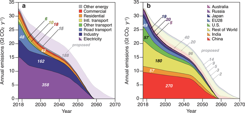
Figure 1 shows future CO₂ emissions from existing and proposed energy and transportation infrastructure by sector (Fig. 1a) and country/region (Fig. 1b). We estimate that cumulative emissions by existing infrastructure, if operated as historically, will be 658 Gt CO₂. Of this total commitment, 54% or 358 Gt CO₂ is anticipated to come from existing electricity infrastructure (mainly power plants), reflecting the large share of annual emissions from electricity infrastructure (46% in 2018) and the long historical lifetimes of generating infrastructure. Another 25% of the total, or 162 Gt CO₂, is related to industrial infrastructure, and 10% or 64 Gt CO₂ is related to the transportation sector (mainly on-road vehicles; Fig. 1a). This difference reveals the effect of infrastructure lifetimes: although industry and road transportation sectors have similar annual CO₂ emissions (6.2 and 5.9 Gt CO₂ in 2018, respectively), vehicle lifetimes are roughly a third as long as industrial capital. Finally, existing residential and commercial infrastructure represent 42 Gt CO₂ and 18 Gt CO₂ of all committed emissions, respectively.

Figure 1 |. Committed CO₂ emissions from existing and proposed energy infrastructure.

Estimates of future CO₂ emissions by industry sector (a; see also Tables S1 and S2) and country/region (b), assuming historical lifetimes and utilization rates. Emissions from existing infrastructure are shown by darker shading, and emissions from proposed power plants (i.e. electricity) are more lightly shaded.

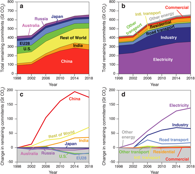
Global committed emissions are now at the apex of a 20-year trend. Between 2002 to 2014, as China emerged as a global economic power, total committed emissions grew at an average annual rate of 9% per year (Extended Data Fig. 1a). Meanwhile, committed emissions related to infrastructure in the U.S. and EU28 have been shrinking since 2006 (Extended Data Fig. 1c). Since 2014, the rate of infrastructural expansion in China and India has also fallen, and committed emissions in China declined by 7% between 2014 and 2018, even as committed emissions in the Rest of World have continued to climb (Extended Data Figs. 1a and 1c). These most recent trends may reflect nascent shifts in China’s economic structure¹⁹ and global trade²⁰, and may be important harbingers of future changes in regions’ annual CO₂ emissions⁹.

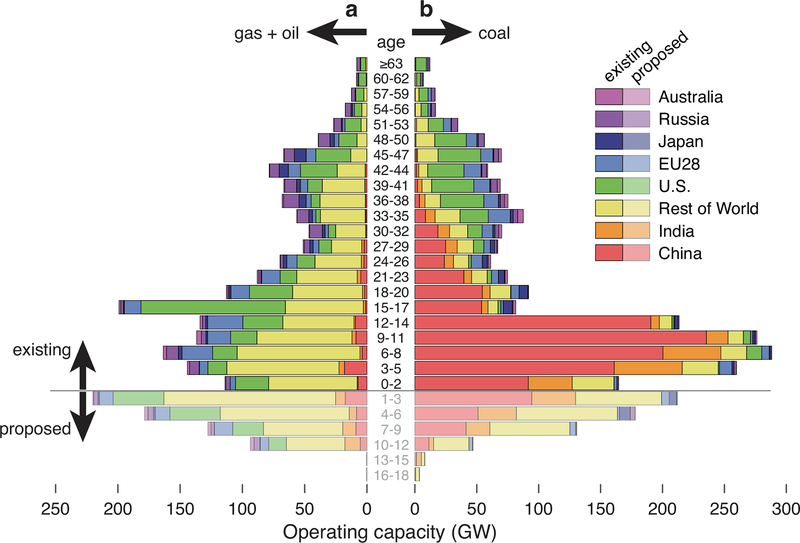
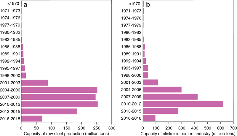
Figure 2 shows the age distribution of electricity generating units worldwide. Overall, the youth of fossil generating units worldwide is striking: 49% of the capacity now in operation worldwide was commissioned after 2004, and this share is 79% and 69% in China and India, respectively. The average age of coal-fired power plants operating in China and India (11.1 and 12.2 years, respectively) is thus much lower than those in the U.S. and the EU28 (39.6 and 32.8 years, respectively; Fig. 2b), with correspondingly longer remaining lifetimes. The predominance of young Chinese infrastructure (which extends to the industrial and transportation sectors; Extended Data Figs. 2 and 3) reflects the scale and speed of the country’s industrialization and urbanization since the turn of the century. As a result, infrastructural inertia is greatest in China, accounting for 41% of all committed emissions (270 Gt CO₂; Fig. 1b). In comparison, infrastructure in India, the U.S., and the EU28 represents much smaller commitments: 57 Gt, 57 Gt, and 49 Gt CO₂, respectively (Fig. 1b; Table S1 in Supporting Information).

Figure 2 |. Age structure of global electricity-generating capacity.

The operating capacity of gas- and oil-fired electricity-generating units (a) and coal-fired units (b) where the youngest units are at the bottom. Lighter shaded bars at the bottom show proposed electricity-generating units according to the year they are expected to be commissioned. Recent trends in Chinese and Indian coal-fired units (red and orange at lower right, respectively) and U.S. gas-fired units (green at left) is apparent. Note that 0 years old means the power units began operating in 2018.

In addition to existing infrastructure, new power plants are being planned, permitted, or constructed, and the committed emissions related to such proposed plants may be estimated^11,12. As of the end of 2018, the best-available data showed 579 GW, 583 GW, and 40 GW of coal-, gas-, and oil-fired generating capacity were proposed to be built over the next several years, respectively (~20% of it in China; Fig. 2). If built and operated as historically, this proposed capacity would represent an additional 188 Gt CO₂ committed: 97 Gt CO₂ from coal-, 91 Gt CO₂ from gas-, oil-, and other-fuel-fired generating units (Table S2).

Together, committed emissions from existing infrastructure and proposed power plants total 846 Gt CO₂ if all proposed plants are built and all infrastructure operated as historically (Fig. 1).

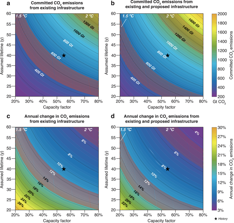
Existing electricity and industry infrastructure accounts for 79% of total committed emissions if operated as historically (i.e. with a 40-year lifetime and 53% utilization rate; Fig. 1a). However, the lifetime and operation of such infrastructure will ultimately depend on the relative costs of competing technologies, in turn influenced by factors such as technological progress and the climate and energy policies in each region^22,26. Figure 3 highlights the sensitivity of committed emissions (Figs. 3a and 3b) and the rate of annual emissions reductions (Figs. 3c and 3d; see Methods) to the assumed lifetime and utilization rates (i.e. capacity factors) of industry and electricity infrastructure (n.b. lifetimes and operation of infrastructure in other sectors are not varied from historical averages), with the star in each panel indicating historical average values. For example, total committed emissions related to existing infrastructure decrease to ~200 Gt CO₂ if lifetimes are and capacity factors decrease to 20 years and 20%, respectively, but increase to almost 1500 Gt CO₂ if lifetimes and capacity factors increase to 60 years and 80%, respectively (Fig. 3a). These ranges of lifetimes and utilization are quite wide, at the low end probably exceeding economic feasibility for recouping capital investments and covering fixed operating and maintenance costs. When proposed power plants are included, total committed emissions over the same range of lifetimes and capacity factors increase to 263–1906 Gt CO₂ (Fig. 3b). Maintaining historical capacity factors, a 5-year difference in the lifetime of existing infrastructure represents roughly 70–100 Gt of future CO₂ emissions (Fig. 3a), or about 90–130 Gt if proposed power plants are included (Fig. 3b). Maintaining historical lifetime and changing the assumed capacity factor by a comparable 9% (e.g., from 46% to 55%) results in roughly the same changes in committed emissions, suggesting these factors have a similar influence.

Figure 3 |. Sensitivity of committed emissions (a, b) and mitigation rates (c, d) to utilization rates and assumed lifetimes.

Contours show estimates of committed emissions related to existing infrastructure (a) and existing infrastructure and proposed power plants (b) when the assumed lifetimes and utilization rates of electricity and industry infrastructure are varied from 20–60 years 20–80%, respectively. Across the same ranges of lifetime and utilization, corresponding annual rates of emission reduction span from 3% to 30% (c and d). Hatched orange and red zones indicate carbon budgets and mitigation rates likely to limit mean warming to 1.5°C and 2°C, respectively (see Methods), and stars denote committed emissions and mitigation rates if existing/and proposed infrastructure is operated as historically.

For comparison, the hatched red and orange zones in Figures 3a and 3b show the Intergovernmental Panel on Climate Change’s (IPCC) most recent estimated ranges of remaining cumulative carbon budgets spanning 50% to 66% probabilities of limiting global warming to 1.5°C and 2°C relative to the preindustrial era⁵. Excluding proposed power plants, our central estimate of committed emissions (658 Gt CO₂; star in Fig. 3a) exceeds the range of the remaining 1.5°C budget (420–580 Gt CO₂)⁵. When proposed plants are included, our estimate of committed emissions (846 Gt CO₂; star in Fig. 3b) is two-thirds of the lower estimates of the 2°C budgets (1170–1500 Gt CO₂)⁵. This suggests that, unless compensated by negative emissions technologies or retrofitted with carbon capture and storage, 1.5°C carbon budgets allow for no new emitting infrastructure and require substantial changes to the lifetime or operation of already existing energy infrastructure (e.g., decreasing lifetimes to <25 years or capacity factors to <30%; Fig. 3a). Moreover, CO₂ emissions related to the extraction and transport of fossil fuels²⁷ and non-energy CO₂ emissions (e.g., due to land use change)²⁸ are not included in our estimates and will further reduce the remaining carbon budgets.

Climate targets have also sometimes been contextualized by the annual rate of emissions reduction they imply. For example, Raupach et al.²⁹ showed, as of 2013, the cumulative carbon budgets likely to avoid 2°C of mean warming implied necessary average annual reductions in global CO₂ emissions (i.e. mitigation rates) of ~6% per year. The hatched areas in Figures 3c and 3d show that such mitigation rates, recalculated from the latest carbon budgets, are about 5% per year for the 2°C budgets (4.5–5.7%) and about 13% per year for 1.5°C budgets (11.4–15.7%). In comparison, the contours in the figure show mitigation rates if no new emitting infrastructure is commissioned (10.1%; star in Fig. 3c) or only proposed power plants but no other emitting infrastructure is commissioned (7.9%; star in Fig. 3d). Again the international targets leave little or no room for new infrastructure if existing plants operate as they have historically (stars) unless fully compensated by negative emissions or retrofitted with carbon capture and storage technologies.

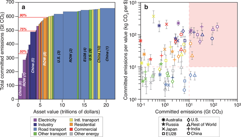
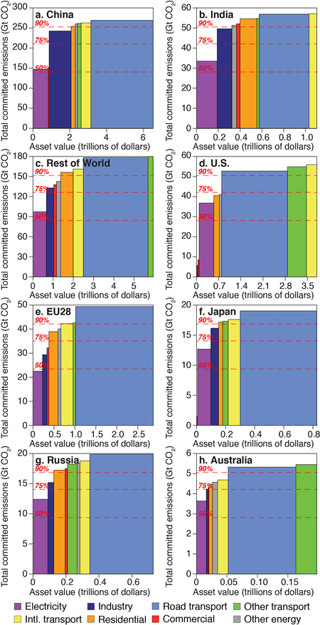
Given the constraints of 1.5°C and 2°C carbon budgets, we also explore the economic value of existing infrastructure relative to its associated committed emissions. Figure 4a highlights the disproportionality of committed emissions per unit asset value. Together power and industry infrastructure (purple and dark blue in Fig. 4a, respectively) represent >75% of total committed emissions (519 of 658 Gt CO₂) but <25% of the estimated economic value of CO₂-emitting energy infrastructure (~$5 trillion of $22 trillion; Extended Data Fig. 4; Table S3; see Methods for details of how asset values were amortized). In contrast, transportation infrastructure, with shorter average lifetimes but high capacity costs and a vast number of discrete units, represents roughly two-thirds of the value of emitting assets and less than 10% of committed emissions (Fig. 4a). This analysis suggests that efforts to reduce committed emissions might cost-effectively target early retirement of electricity and industry infrastructure—despite their often powerful influence on policy and institutions^6,21,22—if non-emitting alternative technologies are affordable: the magnitude of commitments in these sectors is large and a single dollar of asset value is related to >10 kg of future CO₂ emissions (Fig. 4b; red rectangle). Industry and electricity sectors in China represent especially prime targets for unlocking future emissions: nearly half (46%) of these sectors’ committed emissions are associated with Chinese infrastructure (Fig. 4a).

Figure 4 |. Asset value and committed emissions of existing infrastructure.

Rank ordering of CO₂-emitting assets by committed emissions per dollar value reveals large disparities (a; colored by sector). Horizontal red lines in a indicate 50%, 75% and 90% of total committed emissions (658 Gt CO₂) if operated as historically, and the top ten most valuable region-sectors are labeled (see Extended Data Fig. 4 for region-specific versions). Plotting emissions per value (kg CO₂/$) against committed emissions suggests targeted opportunities to “unlock” future CO₂ emissions if alternative technologies are affordable (region-sectors in the pink-shaded quadrant in b; showing 95% confidence intervals with regions denoted by symbols).

Detailed and up-to-date analysis of existing and proposed CO₂-emitting energy infrastructure worldwide reveals incredibly tight constraints of current international climate targets even if no new emitting-infrastructure is ever built. Although climate and energy analysts have emphasized that avoiding 1.5°C of warming, for example, remains “technically possible”⁵, our results lend vivid context to that possibility: we would have a reasonable chance of achieving the 1.5°C target with (1) a global prohibition of all new CO₂-emitting devices—including many or most of the already proposed fossil fuel-burning power plants, and (2) substantial reductions in the historical lifetimes and/or utilization rates of already existing industry and electricity infrastructure.

Barring such radical changes, the global climate goals adopted in the Paris Agreement are already in jeopardy and may be contingent upon widespread retrofitting of existing emitting infrastructure with carbon capture and storage technologies (which retrofits would be tremendously expensive³⁰), large-scale deployment of negative emissions technologies¹⁶, and/or solar radiation management⁴. On the other hand, our results suggest that the level of future warming in excess of the Paris targets is largely dependent on infrastructure that has not been built yet (Extended Data Fig. 5).

Some important caveats and limitations apply to our findings. The trajectory of future emissions depicted in Figure 1 represents a scenario in which existing (and proposed) emitting infrastructure “ages out,” and no new emitting infrastructure is ever commissioned. These constraints are not intended as realistic; rather, they allow us to isolate and quantify infrastructural—and related economic—lock-in of energy-related emissions²². Indeed, technological trends and climate-energy policies that encourage growth in renewable electricity (e.g., solar and wind) may lead to earlier than historical retirements of existing fossil fuel power plants in some regions, although recent growth of renewable generation has not always displaced fossil generation¹⁸. It is also instructive to compare our estimates of committed emissions to plausible energy-emissions scenarios generated by much more sophisticated (but less transparent) IAMs that calculate infrastructure lifetimes and capacity factors endogenously. For example, a recent IAM study of 1.5°C scenarios found that large-scale carbon dioxide removal may be necessary to compensate for “residual” emissions from long-lived and difficult-to-decarbonize sectors of the energy system (e.g., freight, aviation, and shipping⁴)³¹.

The size of carbon budgets associated with a given temperature target is also a complicated matter that is sensitive to a host of factors such as climate sensitivity and non-CO₂ emissions^14,15. The budgets from the recent IPCC Special Report are estimates of cumulative net global anthropogenic CO₂ emissions from the start of 2018 until net-zero global CO₂ emissions are achieved (i.e. climate is stabilized) with a 50–66% probability of limiting an increase of mean near-surface air temperatures to 1.5°C or 2°C with limited (<0.1°C) or no overshoot⁵ (see Methods for further discussion).

Although ambitious climate targets such as 1.5°C may help to motivate and accelerate the transition toward net-zero energy systems, their feasibility is often evaluated by the existence of consistent scenarios from IAMs. However, these models have been used to analyze a very large possibility space, and some scenarios may thus reflect aspirational trajectories of energy demand or technological progress and scale whose likelihood may be difficult to evaluate^32,33. Our data-driven assessment of existing, operating, and valuable energy infrastructure may therefore help to elucidate the infrastructural and economic implications of such targets, and also help to identify targeted regional and sectoral opportunities for unlocking future CO₂ emissions.

Methods

Committed emissions from existing and proposed infrastructure

We extend the approach of Davis et al⁹ to quantify the committed emissions from existing energy infrastructure by integrating more detailed and up-to-date data of energy infrastructure available, including country- and duty-specific vehicle sales data, and unit-level details of global power plants and Chinese cement kilns and blast furnaces^10,34–39. We also estimate committed emission from proposed power plants by collecting all proposed power generators from the latest available databases^34,37, in recognition of substantial changes in the pipeline of planned power plants (especially coal) in recent years³⁴. Energy infrastructure as quantified in this study is categorized into eight sectors: (1) electricity, (2) industry, (3) road transport, (4) other transport, (5) international transport, (6) residential, (7) commercial and (8) other energy infrastructure (see Tables S4 and S5).

Electricity infrastructure

Emissions from electricity infrastructure in this study include all emissions under category 1A1 of the IPCC’s Revised Guidelines⁴⁰. Electricity infrastructure here mainly includes main activity electricity and heat production (1A1a), and petroleum refining (1A1b), as well as manufacturing of solid fuels and other energy industries (1A1c) (Table S5).

Emissions intensities.

Previously, we built and published a comprehensive global thermal power plants database in 2010 (named GPED) by integrating high-quality national databases (China, India, and the U.S.)¹⁰. Here we update the GPED database to the year 2018 (named GPED-2018) using the latest power plant database from China (CPED)³⁶ and the Platts World Electric Power Plant (WEPP) database for other regions³⁷, including all retired and operating units through the end of 2018. We obtain data and estimates of unit-based CO₂ emission intensity (i.e. gCO₂/kwh) for all units that were operating in 2010 from GPED-2010. For units retired prior to 2010 or commissioned since 2010, we estimate unit-level CO₂ emission intensity by the methods of Davis et al⁹ based on the Carbon Monitoring for Action (CARMA) database³⁵ (for older units) or else use national or regional average CO₂ emission intensity for units with the same fuel type and similar nameplate capacity. As prior studies have done, we assume these emissions intensities are constant over a unit’s lifetime^8,9.

Assumed lifetime.

In the resulting GPED-2018, global average lifetimes of retired coal-, nature gas-, and oil-fired power units is 35.9, 37.1, and 33.9 years, respectively. Consistent with prior study⁹ have done, we simplify these ranges to a single reference lifetime of 40 years for all electricity-generating units for our “as historically” case, and show the sensitivity of committed emissions to this assumption in Figure 3. When units already operating beyond their assumed lifetime, these units are randomly retired over the next 5 years in order to avoid unrealistically abrupt changes in emissions between 2018 and 2019.

In addition, we assume that the age structure and lifetime of autoproducers (industrial and commercial facilities which generate their own electricity on-site)⁴⁰ and other energy industries are similar to the main activity power plants in each region. Therefore, committed emissions from existing electricity infrastructure are quantified by employing the survival curves derived from main activity power plants, scaled to include these other types of electricity infrastructure using country-level electricity emissions totals in 2018 from the International Energy Agency (IEA). It is noted that the country-level CO₂ emissions from fossil fuel combustions for 2018 were derived from multiplying country-level CO₂ emissions in 2016 by projected change rates during 2016–2018 due to data availability⁴¹.

Finally, we quantify the cumulative future CO₂ emissions from proposed power plants by the same procedure (assuming historical average unitization rates and lifetimes) using a database of proposed coal-fired units that has been developed by CoalSwarm³⁴ and the planned units fired with other fossil fuels from the Q4 2018 WEPP database³⁷.

Industry infrastructure

Industrial emissions in this study include all emissions under category 1A2 of the IPCC’s Revised Guidelines⁴⁰. For all countries but China, we estimate cumulative future emissions from industry infrastructure using country-level emissions data for the year 2018 obtained from the IEA and assuming that the age distribution and survival curves of each region’s industry infrastructure is consistent with its electricity infrastructure. To derive China’s industrial survival curves, we use unit-level details of cement kilns and blast furnaces (iron & steel) currently operating in China (Extended Data Fig. 2), obtained from China’s Ministry of Ecology and Environment (MEE) (unpublished data, hereinafter refer to as the MEE database).

The detailed data of Chinese infrastructure represent an important improvement in the current study over prior estimates of committed emissions, as we China alone accounts for ~47% of total industrial emissions⁴¹. In particular, the iron/steel and non-metallic minerals (e.g., cement and glass) industries account for ~50% of all industrial CO₂ emissions in recent years⁴¹, and China produced 49.6% of the world’s raw steel and 57.3% of the world’s cement in 2016⁴². The unit-level data of China’s industrial infrastructure thus substantially decreases uncertainty of committed industry emissions by alleviating the need for assumptions related to almost half of global industry infrastructure (i.e. 9.0% of global CO₂ emissions from all sources⁴¹). Moreover, we observed that the age distributions of electricity and industry infrastructure in China are quite similar (Extended Data Fig. 6), which lends support to our assumption that this is the case in other regions where we lack detailed data of industrial infrastructure.

Transportation infrastructure

Transport emissions in this study include all emissions under category 1A3 of the IPCC’s Revised Guidelines⁴⁰, which includes emissions from road transport, other transport and international transport (Tables S4 and S5).

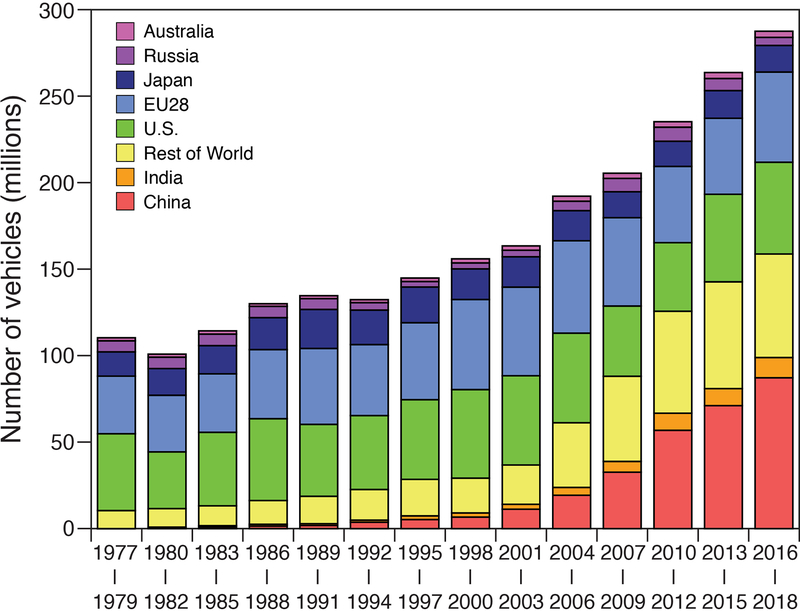
Cumulative future emissions from road transport were calculated following the approach in Davis et al.⁸ and further updating the activity rates with updated country-, region-, and duty-specific vehicle sales data^38,39 (i.e. 18% of global CO₂ emissions from all sources⁴¹). Specifically, we use the number, class, and vintage of motor vehicles sold during 1977–2017 from 40 major countries and regions^38,39 (information for 2018 was derived by projecting 2016–2017 rates of change one additional year; Extended Data Fig. 3). We then estimate the number of vehicles remaining on the road over time using class- and model year-specific survival rates of U.S. and Chinese vehicles to represent developed and developing countries or regions due to data availability, respectively^43,44. We then calculate annual vehicle emissions based on the average miles driven per year (MPY) per vehicles by class and carbon emission factors of 10.23 and 11.80 kg CO₂ per gallon of gas and diesel, respectively, and scale our estimated emissions to match country-level road transport emissions in 2018 as reported by the IEA⁴¹.

“Other transportation” infrastructure includes existing aviation, rail, pipeline, navigation and other non-specified transport. International transport infrastructure includes international marine bunkers and international aviation bunkers in this work (Table S4). Again, we follow Davis et al.⁸, estimating cumulative future CO₂ emissions from existing other and international transport using country-level emissions data of 2018 from IEA, and assuming lifetimes and age distributions similar to motor vehicle fleets in each country/region.

Residential, commercial and other energy infrastructure

Residential and commercial emissions are included under category 1A4 of the IPCC’s Revised Guidelines⁴⁰, and “Other energy” emissions include, e.g., emissions from agriculture, forestry, fishing, and aquaculture under category 1A4 as well as and stationary, mobile, and multilateral operations under category 1A5 of the IPCC’s Revised Guidelines. Cumulative future emissions from this infrastructure were calculated using country-level emissions data of 2018 derived from the IEA⁴¹, and assuming age distributions and lifetimes of residential, commercial and other energy infrastructure in each region were similar to electricity infrastructure in the same region in the absence of better information.

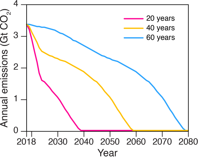
The least-supported methodological assumptions we make thus concern this residential, commercial and other energy infrastructure (~10% of total fossil fuel CO₂ emissions in 2016⁴¹), where we lack any unit-level data. In order to test the sensitivity of total committed emissions from this infrastructure, we performed additional analyses of different assumed lifetimes. We found the committed emissions from residential, commercial, and other energy infrastructure are 29, 74, and 135 Gt CO₂ when lifetimes of 20, 40, and 60 years are assumed, respectively (Extended Data Fig. 7). That is, our estimates of total committed emissions from all existing energy infrastructure decrease by 7% (to 613 Gt CO₂) if lifetimes of residential, commercial, and other energy infrastructure are assumed to be 20 years, and increase by 9% (to 719 Gt CO₂) if the lifetimes are assumed to be 60 years. In comparison to the carbon budgets associated with targets of 1.5 °C and 2 °C, these are relatively small effects, and not substantial enough to affect the main conclusions of our study.

Comparison of cumulative future emissions estimates

Other studies have analyzed committed emissions of various infrastructure in different ways, as mentioned in the text and summarized in Extended Data Table 1^8,9,11–13.

For example, both Edenhofer et al.¹¹ and Pfeiffer et al.¹² reported committed emissions related to existing and planned power plants using 2016 data. Although the latter analyzed committed emissions of all fossil electricity infrastructure¹², the former focused particularly on coal-fired units¹¹. Importantly, the 2018 data used in the current study reveals that substantial cancellations of proposed plants have occurred over the intervening two years: whereas the previous studies estimated ~150 Gt CO₂ and 210 Gt CO₂ were committed by proposed coal plants, we estimate only ~100 Gt CO₂, 50–100 Gt CO₂ less, respectively (or 10–20% of the remaining carbon budget consistent with 1.5°C, respectively). Moreover, our study contains more detailed estimates of regional commitments and the sensitivity of these commitments to assumed lifetime and capacity factor.

Most recently, Smith et al.¹³ estimated the global warming related to committed emissions using a reduced-complexity climate model (FaIR). Their study also included estimates of committed emissions from all sectors, but these relied on past estimates of the age distribution of fossil fuel infrastructure and an idealized, linear phase-out of such infrastructure¹³. Because turnover of infrastructure has decreased the median age of electricity generating capacity in many regions (Fig. 2), our estimates of electric power sector commitments (358 Gt CO₂) are ~13 Gt CO₂ greater than those used by Smith et al¹³ (345 Gt CO₂). Our data-driven approach also permits region-specific results, analysis of the trend in commitments over time, inclusion of proposed power plants, and an assessment of the economic value of underlying infrastructures. Yet, because Smith et al.’s estimates of CO₂ emissions committed by other infrastructure are larger than our bottom-up estimates (Extended Data Table 1), the overall estimate reached by their idealized approach (715 Gt CO₂) is nonetheless similar to that of the current study (658 Gt CO₂).

In turn, Smith et al.¹³ assess the global climate responses to the committed CO₂ and conclude that the world is not yet committed to 1.5°C¹³. However, it is difficult to directly compare the magnitude of the CO₂ emissions in Smith et al.’s phase-out scenarios with the SR1.5 carbon budgets for two reasons: First, although SR1.5 also used the FaIR model in its procedure of evaluating non-CO₂ forcing, it did not use the FaIR model’s transient climate response to cumulative emissions (TCRE), which is smaller and would have led to considerably larger carbon budgets. Second, the mitigation scenarios evaluated by Smith et al. also assumed that non-CO₂ emissions are completely phased out in parallel to CO₂, while the integrated assessment model scenarios on which the SR1.5 report’s non-CO₂ forcing (and carbon budgets) are based do not completely eliminate non-CO₂ emissions this century⁴⁵.

Variation of utilization rates and assumed lifetimes

As described above, cumulative future committed emissions from electricity and industry infrastructure depend on utilization rates and assumed lifetimes. The longer the assumed lifetime and higher the utilization, the greater the estimate of committed emissions will be. In this study, we therefore test the sensitivity of committed emissions to assumed lifetimes and utilization rates of energy and industry infrastructure across lifetimes from 20 to 60 years and utilization rates of 20% to 80%.

Remaining carbon budgets to limit mean warming to 1.5 and 2 °C

As described in the text and discussed in recent literature, the size of carbon budgets associated with a given temperature target is a complicated matter that is sensitive to a host of factors^14,15, including (1) whether the budget reflects cumulative net emissions until the temperature target is exceeded or cumulative net emissions that limits global temperature increase to below the target (i.e. climate is stabilized), (2) whether there can be a temporary overshoot of the temperature target (and by how much)⁴⁶, (3) the climate responses to CO₂ and non-CO₂ forcings⁴⁷, (4) the magnitude and Earth system response to negative emissions⁴⁸, (5) how global temperature is calculated, (6) the pre-industrial baseline used⁴⁹, (7) whether Earth system feedbacks such as permafrost thawing are included^50–53, and (8) future emissions of non-CO₂ greenhouse gases and aerosols^54,55.

The magnitude of non-CO₂ forcing is particularly relevant to assessments of committed emissions because non-CO₂ forcing is inversely related to the remaining carbon budget^54,55, and because some non-CO₂ greenhouse gases and aerosols are directly related to the current energy system (e.g., fugitive methane⁵⁶) or are co-emitted with CO₂ by fossil fuel-burning infrastructure. Other large sources of non-CO₂ gases and aerosols exist outside of the energy system, such as agriculture⁵⁷. For the SR1.5 budgets, non-CO₂ forcing was estimated using integrated assessment model scenarios and a pair of reduced-complexity climate models (MAGICC and FaIR), with substantial uncertainties associated with both scenario variations (±250 Gt CO₂) and climate responses (-400 to 200 Gt CO₂) for the 1.5°C budget⁵. Non-CO₂ greenhouse gases and aerosols decline but do not reach zero in any of the scenarios assessed by the SR1.5 report. In contrast, the recent study by Smith et al. modeled the complete phase-out of non-CO₂ emissions in parallel with energy-related CO₂ emissions, a formidable scenario that was found to have a high probability (64%) of limiting warming to 1.5°C¹³.

In this study, we compare our estimates of committed emissions to the SR1.5 budgets⁵. As defined by the recent SR1.5 report, remaining carbon budgets are the cumulative net global anthropogenic CO₂ emissions from a given start date (January 1, 2018) to the year in which such emissions reach net zero that would result, at some probability, in limiting global warming to a given level⁵. By this definition, budgets are not simply cumulative emissions until the time when mean temperature exceeds a given threshold¹⁴, but rather what have been called “threshold avoidance” or called “stabilization” budgets. The SR1.5 budgets were derived from the transient climate response to cumulative CO₂ emissions in climate model simulations that have been further adjusted to include additional climate forcing related to non-CO₂ greenhouse gases and aerosols⁴⁵. They do not include Earth system feedbacks (which the report suggests could reduce the remaining budgets by 100 Gt CO₂ over the century).

However, as remaining budgets associated with mean surface warming of 1.5°C dwindle, uncertainties in transient climate response to CO₂ emissions^15,47 and the current and future non-CO₂ forcing loom large^53–55. In order to make our results as useful, transparent, and comparable as possible, we report positive, CO₂-only commitments from existing and proposed fossil fuel-burning infrastructure and compare to these to the remaining (stabilization) carbon budgets reported by the SR1.5 report to give a 50–66% probability of limiting warming to 1.5°C and 2°C with little (0.1°C) or no overshoot: 420–580 Gt CO₂ and 1170–1500 Gt CO₂, respectively (See Table 2.2 in ref.⁵). Thus, if not offset by negative emissions, the total committed emissions we estimate if existing infrastructure operates as it has historically (i.e. 658 Gt CO₂) would make it likely that global temperatures will exceed 1.5°C unless the remaining carbon budgets in the SR1.5 are substantially wrong. For example, the climate response to CO₂ could be less than expected based on the climate model simulations the SR1.5 assessed and/or non-CO₂ forcing in the future could be much less than it is on average in the integrated assessment model scenarios that were assessed by the SR1.5. Indeed, Smith et al.¹³ analyzed a future where both are true.

Estimates of the annual rate of emission reductions

We estimate annual rate of emissions reduction (“mitigation rates”) following Raupach et al (2014)²⁹:

$$\mathrm{f}\left(\mathrm{t}\right)=f_0\left(1+\left(r+m\right)t\right)$$

where f(t) is the emissions at time t, f₀ is the emissions at the start of mitigation (t = 0), r is an initially linear growth rate, and r and m both have units of per year. When the necessary annual rate of emission reductions to meet quota q from t=0 onward (with emission time T = q/f0), we estimate the annual rate of emission reductions, m, as:

$$\mathrm{m}\left(\mathrm{q}\right)=\frac{1+\sqrt{1+rq/f_0}}{q/f_0}=\frac{1+\sqrt{1+r/T}}{T}$$

We use initial emissions f₀ at 2018 and growth rates r averaged over 2013–2018. Therefore, f₀= 32.7 Gt and r = 0.028% used obtained from IEA⁴¹ when estimating mitigation rates under different cumulative CO₂ emissions, which we assumed to be equivalent to the carbon quota, q.

Estimates of asset value from existing infrastructure

We estimate the asset value by sector and by country/region using the following equation:

$${\mathrm{A}\mathrm{V}}_{i,s}=\sum _{n=PY-LT}^{PY}\sum _y\left({\mathrm{T}\mathrm{C}}_{i,\mathrm{ }s,n,y}\times {\mathrm{C}\mathrm{C}}_{i,\mathrm{ }s,n,y}\times \left(\left(1-\mathrm{R}\mathrm{V}\right)\times {\mathrm{D}\mathrm{R}}_{i,s,n,y}+RV\right)\right)$$

where i, s, n, y represents country/region, sector, years, and combustion/production technology, AV represents asset value, TC represents equivalent total capacity, CC represents capital costs, RV represents the ratio of residual value, and 5% is applied for all the infrastructure; DR represents depreciation rate, PY represents present year, referring 2018 in this study.LT represents lifetimes.

We adopt sector-dependent method, and apply straight-line and geometric models for different infrastructure, as shown in Table S6. Data on capital costs used to estimate the asset value was collected from previous literature^{12,21,23–25,58,59} and various reports^60–64. Wherever possible, we use interannual and national average capital costs for different combustion/production technology and equipment. Where an interannual and national averages were not available, we instead use an average of all the countries in the same region where capital cost data were available.

Electricity infrastructure

We estimate the total value of fossil fuel electricity-generating assets according to each unit’s power generating capacity (kW) and age, as well as fuel- and technology-specific capital costs ($/kW).

The assumed lifetime of coal power plants is 40 years. Although plants can operate for considerably longer periods, shutting down a plant after its assumed lifetime will not result in any stranded capital investment since the initial capital cost will have been fully paid²⁴. Thus, our estimates only include the asset value of operating electricity-generating units that are now less than 40 years old. Unit-level details of electricity-generating technologies were obtained from GPED-2018 database.

In addition, part of committed CO₂ emissions in electricity infrastructure are from heating plants. The asset value of combined heat and power (CHP) plants have been evaluated along with other power plants, but we estimate the asset value of individual heating plants separately, using IEA data on heating output (TJ)^65,66 to estimate the capacity of such heating plants and converting this to an equivalent power capacity (GW) assuming they operate with the average utilization rates of power generating units in the same region. Table S6 summarizes the assumptions of estimating asset value of individual heating plants.

Industrial infrastructure

Industrial infrastructure includes various facilities and systems from different sub-industrial sectors (Tables S4 and S5). Considering the difficulty of collecting the operating capacity for all the sub-industrial sectors, we estimate the value of industry infrastructure as the combined asset values of cement, iron and steel plants, and industrial boilers. As described above, only the asset value for cement, iron and steel capacity operating less than 40 years was estimated in this work. Asset value from cement, iron and steel industry are quantified through total capacity and capital investment per unit (Table S6).

We estimate total capacities (t/h) of industrial boilers at country- or region-level by fuel type by through total energy consumptions obtained from IEA^65,66. The utilization rates of industrial boilers are assumed to be the same as the average utilization rate of electricity infrastructure. The related assumptions are shown in Table S6.

Transport infrastructure

We quantify the value from road transport, other transport and international transport assets separately. For road transport infrastructure, we estimate asset value by number of annual vehicle sales, annual average new car prices, and a depreciation rate function. The data sources of number of annual vehicle sales is described above, and we further collect annual average new car prices by vehicle type and country/region³⁹. Because depreciation rates tend to be considerably lower in developing countries than industrialized countries⁶⁷, we adopt different depreciation rate functions for developing and developed countries⁶⁷.

For international transport infrastructure, we estimate the value of international ships and international airplanes. Due to limited data availability, we use the same approach as with heating infrastructure, basing our estimates on the total energy consumption (fuels) for international aviation and international navigation from the IEA, and converting to the number of reference narrow-body aircraft and standardized international freight ships by such fuel consumption. Specifically, we assume 2 million-km/year per aircraft and 149 MJ/airplane-km for reference narrow-body aircrafts²¹ (Table S6); 940 million annual ton-km and an average ship energy intensity of 0.125 MJ/ton-km for international freight ships²¹. We use the same total average depreciation rates for international transport as we do for road transport infrastructure.

We use a similar approach for other transport (i.e. domestic ships, domestic airplanes, and non-specific transport), adopting the same assumptions applied in the international transport for domestic ships and domestic airplanes. For non-specific transport, we quantify asset values by converting to the number of conventional diesel heavy-duty freight truck. The corresponding assumptions are shown in Table S6.

Residential, commercial and other energy infrastructure

We quantify the asset values of residential, commercial and other energy infrastructure separately using sector- and fuel-specific energy consumption data from the IEA^65,66.

Residential and commercial infrastructure use energy for space heating, heating water, and cooking. Other energy infrastructure includes uses of energy for agriculture, fishing and other activities. Given very limited data, we quantify the value of residential and commercial infrastructure by according to an equivalent capacity of normalized space heating units, water heating units, and cooking equipment. In the other energy infrastructure, we quantified the asset value by converting to normalized agriculture machines, fishing boats and boilers. We then apply the total average depreciation rates of electricity infrastructure to these residential, commercial and other energy infrastructures.

Uncertainty estimated

Our estimates of asset values are subject to uncertainty due to incomplete knowledge of operating capacities, their age structure, and the capital costs per unit. In order to more completely assess uncertainties in our results, we perform a Monte Carlo analysis of asset values by sector and by country/region in which we vary key parameters according to ranges in the literature^58,68,69 and collected capital costs data above. The error bars shown in Figure 4 depict the results of this analysis, showing the lower and upper bounds of a 95% confidence interval (CI) around our central estimate. The Monte Carlo simulation uses specified probability distributions for each input parameter (e.g., capital cost per unit, and the ratio of residual value) to generate random variables⁶⁸. The probability distribution of asset value is estimated according to a set of runs (n=10,000) in a Monte Carlo framework with probability distributions of the input parameters. The ranges of sector- and -region-parameter values vary in part due to the quality of their statistical infrastructure⁶⁹. Table S7 summarizes the probability distributions of the asset value estimation-related parameters.

Data availability

The numerical results plotted in Figures 1–4 are provided with the manuscript. Our analysis relies on six different datasets, each used with permission and/or by license. Five are available from their original creators: (1) the GPED database: http://www.meicmodel.org/dataset-gped.html, (2) Platt’s WEPP database: https://www.spglobal.com/platts/en/products-services/electric-power/world-electric-power-plants-database, (3) the CARMA database: http://carma.org/, (4) the CoalSwarm database: https://endcoal.org/tracker/, and (5) vehicle sales data: https://www.statista.com/markets/419/topic/487/vehicles-road-traffic/. The sixth dataset includes unit-level data of Chinese iron, steel and cement infrastructure which we obtained directly from the Chinese Ministry of Ecology and Environment. We do not have permission to share the raw data, but we provide it in an aggregated form (Extended Data Figure 2).

Extended Data

Extended Data Figure 1 |. Changes in remaining commitments from existing energy infrastructure.

Estimates of future CO₂ emissions every four years by industry sector (a) and country/region (b) from 1998 to 2018 (1998, 2002, 2006, 2010, 2014, and 2018), assuming historical lifetimes and utilization rates. Panels (c) and (d) show corresponding changes in remaining commitments by industry sector (c) and country/region (d).

Extended Data Figure 2 |. Age structure of Chinese major industrial capacity.

The operating capacity of raw steel in iron and steel industry (a) and clinker in cement industry (b) where the youngest units are at the bottom.

Extended Data Figure 3 |. Age structure of currently road transport infrastructure.

This figure shows the population of vehicle sales by country/region.

Extended Data Figure 4 |. Asset value and committed emissions of existing infrastructure.

Cumulative committed CO₂ emissions in the order of committed emission per value (kg CO₂ per $) (from high to low) by country/region and sector. Dash horizontal lines indicate 50%, 75% and 90% of total committed emissions if operated as historically, respectively.

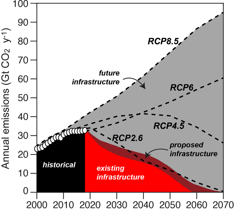
Extended Data Figure 5 |. Annual emissions from existing, proposed and future infrastructure.

This figure shows historical CO₂ emissions from fossil fuel energy infrastructure (black area), and future CO₂ emissions from existing (red area) and proposed energy infrastructure (dark red area), as well as future infrastructure (dark grey area) under representative concentration pathways (RCPs: RCP8.5, RCP6, RCP4.5, and RCP2.6).

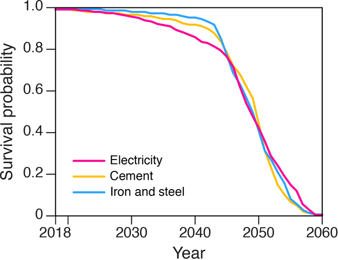
Extended Data Figure 6 |. Survival curves of power and major industries in China.

This figure shows survival curves of power sector (peachblow line), cement industry (orange line), and iron and steel industry (blue line) in China under the assumption of 40-year lifetimes.

Extended Data Figure 7 |. Annual emissions from residential, commercial, and other energy infrastructure.

This figure shows future annual CO₂ emissions from residential, commercial, and other energy infrastructure under the assumptions of 20- (peachblow line), 40- (orange line), and 60-year (blue line) lifetimes.

Extended Data Table 1 |. Comparing commitments.

Comparison of committed emissions by sector estimated in the current study and prior studies. Note that in some cases, the totals may not correspond to the sum of underlying sectors due to rounding.

		Davis et al. (2010)8		Davis and Socolow (2014)9		Edenhofer et al. (2018)11		Pfeiffer et al. (2018)12		Smith et al. (2019)13		This study
		Gt CO2	Year of dataset	Gt CO2	Year of dataset	Gt CO2	Year of dataset	Gt CO2	Year of dataset	Gt CO2	Year of dataset	Gt CO2	Year of dataset
Existing	Electricity	224	2009	307	2012	-	-	308	2016	345 (261–451)	2009**	358 (240–493)	2018
	Coal		2009	206	2012	190	2016	220	2016	-	-	260 (175–358)	2018
	Gas, oil, and other fuels		2009	100	2012	-	-	88	2016	-	-	98 (65–135)	2018
	Industry	104	2009			-	-	-	-	154 (117–191)	2009	162 (110–219)	2017
	Transport	116	2009			-	-	-	-	92 (73–110)	2017	64 (53–75)	2017
	Residential, commercial, and other energy	53	2009			-	-	-	-	121 (91–158)	2009*	74 (52–105)	2018
	All Sectors	496 (282–701)				-	-	-	-	715 (546–909)	-	658 (455–892)	-
Proposed	Electricity					-	-	271	2016	-	-	188 (142–234)	2018
	Coal					150	2016	210	2016	-	-	97 (74–121)	2018
	Gas, oil, and other fuels					-	-	61	2016	-	-	91 (68–113)	2018
All Sectors + Proposed Electricity												846 (597–1,126)

^*The range represents the committed emissions estimated under the assumptions of 30–50 years’ lifetimes for all the sectors except transportation sector (12–18 years’ lifetimes).

^**The age distribution of infrastructure was assumed to be the same as 2009, but annual emissions from the infrastructure was adjusted up to 2018 levels.

References

- 1.Matthews HD & Caldeira K Stabilizing climate requires near-zero emissions. Geophys. Res. Lett 35, L04705 (2008). [Google Scholar]
- 2.Meinshausen M et al. Greenhouse-gas emission targets for limiting global warming to 2 °C. Nature 485, 1158–1162 (2009). [DOI] [PubMed] [Google Scholar]
- 3.Rogelj J et al. Zero emission targets as long-term global goals for climate protection. Environ. Res. Lett 10, 10 (2015). [Google Scholar]
- 4.Davis SJ et al. Net-zero emissions energy systems. Science 360, eaas9793 (2018). [DOI] [PubMed] [Google Scholar]
- 5.Rogelj J et al. Mitigation pathways compatible with 1.5°C in the context of sustainable development In: Global warming of 1.5°C. An IPCC Special Report on the impacts of global warming of 1.5°C above pre-industrial levels and related global greenhouse gas emission pathways, in the context of strengthening the global response to the threat of climate change, sustainable development, and efforts to eradicate poverty [Masson-Delmotte V, Zhai P, Pörtner HO, Roberts D, Skea J, Shukla PR, Pirani A, Moufouma-Okia W, Péan C, Pidcock R, Connors S, Matthews JBR, Chen Y, Zhou X, Gomis MI, Lonnoy E, Maycock T, Tignor M, Waterfield T (eds.)]. In Press. [Google Scholar]
- 6.Unruh GC & Carrillo-Hermosilla J Globalizing carbon lock-in. Energ. Policy 34, 1185–1197 (2006). [Google Scholar]
- 7.Matthews HD, Gillett NP, Stott PA & Zickfeld K The proportionality of global warming to cumulative carbon emissions. Nature 459, 829–832 (2009). [DOI] [PubMed] [Google Scholar]
- 8.Davis SJ, Caldeira K & Matthews HD Future CO2 Emissions and Climate Change from Existing Energy Infrastructure. Science 329, 1330–1333 (2010). [DOI] [PubMed] [Google Scholar]
- 9.Davis SJ & Socolow RH Commitment accounting of CO2 emissions. Environ. Res. Lett 9, 084018 (2014). [Google Scholar]
- 10.Tong D et al. Targeted emission reductions from global super-polluting power plant units. Nat. Sustain 1, 59–68 (2018). [Google Scholar]
- 11.Edenhofer O, Steckel JC, Jakob M & Bertram C Reports of coal’s terminal decline may be exaggerated. Environ. Res. Lett 13, 024019 (2018). [Google Scholar]
- 12.Pfeiffer A, Hepburn C, Vogt-Schilb A & Caldecott B Committed emissions from existing and planned power plants and asset stranding required to meet the Paris Agreement. Environ. Res. Lett 13, 054019 (2018). [Google Scholar]
- 13.Smith CJ et al. Current fossil fuel infrastructure does not yet commit us to 1.5 °C warming. Nat. Commun 10, (2019). [DOI] [PMC free article] [PubMed] [Google Scholar]
- 14.Rogelj J et al. Differences between carbon budget estimates unravelled. Nat. Clim. Change 6, 245–252 (2016). [Google Scholar]
- 15.Peters GP Beyond carbon budgets. Nat. Geosci 11, 378–380 (2018). [Google Scholar]
- 16.Gasser T, Guivarch C, Tachiiri K, Jones CD & Ciais P Negative emissions physically needed to keep global warming below 2 °C. Nat. Commun 6, (2015). [DOI] [PubMed] [Google Scholar]
- 17.UNFCCC. Adoption of the Paris Agreement Report No. FCCC/CP/2015/L.9/Rev.1, http://unfccc.int/resource/docs/2015/cop21/eng/l09r01.pdf (UNFCCC, 2015). [Google Scholar]
- 18.Le Quéré C et al. Drivers of declining CO2 emissions in 18 developed economies. Nat. Clim. Change 9, 213–217 (2019). [Google Scholar]
- 19.Guan D et al. Structural decline in China’s CO2 emissions through transitions in industry and energy systems. Nat. Geosci 11, 551–555 (2018). [Google Scholar]
- 20.Meng J et al. The rise of South–South trade and its effect on global CO2 emissions. Nat. Commun 9, 1871 (2018). [DOI] [PMC free article] [PubMed] [Google Scholar]
- 21.Erickson P, Kartha S, Lazarus M & Tempest K Assessing carbon lock-in. Environ. Res. Lett 10, 084023 (2015). [Google Scholar]
- 22.Seto KC et al. Carbon Lock-In: Types, Causes, and Policy Implications. Annu. Rev. Environ. Resour 41, 425–452 (2016). [Google Scholar]
- 23.Bertram C et al. Carbon lock-in through capital stock inertia associated with weak near-term climate policies. Technol. Forecast. Soc. Change 90, 62–72 (2015). [Google Scholar]
- 24.Johnson N et al. Stranded on a low-carbon planet: Implications of climate policy for the phase-out of coal-based power plants. Technol. Forecast. Soc. Change 90, 89–102 (2015). [Google Scholar]
- 25.Pfeiffer A, Millar R, Hepburn C & Beinhocker E The ‘2°C capital stock’ for electricity generation: Committed cumulative carbon emissions from the electricity generation sector and the transition to a green economy. Appl. Energy 179, 1395–1408 (2016). [Google Scholar]
- 26.Wilson C, Grubler A, Bauer N, Krey V & Riahi K Future capacity growth of energy technologies: are scenarios consistent with historical evidence? Clim. Change 118, 381–395 (2013). [Google Scholar]
- 27.Burnham A et al. Life-Cycle Greenhouse Gas Emissions of Shale Gas, Natural Gas, Coal, and Petroleum. Environ. Sci. Technol 46, 619–627 (2012). [DOI] [PubMed] [Google Scholar]
- 28.Arneth A et al. Historical carbon dioxide emissions caused by land-use changes are possibly larger than assumed. Nat. Geosci 10, 79–84 (2017). [Google Scholar]
- 29.Raupach MR et al. Sharing a quota on cumulative carbon emissions. Nat. Clim. Change 4, 873–879 (2014). [Google Scholar]
- 30.Rubin ES & Zhai H The Cost of Carbon Capture and Storage for Natural Gas Combined Cycle Power Plants. Environ. Sci. Technol 46, 3076–3084 (2012). [DOI] [PubMed] [Google Scholar]
- 31.Luderer G et al. Residual fossil CO2 emissions in 1.5–2 °C pathways. Nat. Clim. Change 8, 626–633 (2018). [Google Scholar]
- 32.Rogelj J et al. Energy system transformations for limiting end-of-century warming to below 1.5 °C. Nat. Clim. Change 5, 519–527 (2015). [Google Scholar]
- 33.Grubler A et al. A low energy demand scenario for meeting the 1.5 °C target and sustainable development goals without negative emission technologies. Nat. Energy 3, 515–527 (2018). [Google Scholar]
- 34.Shearer C et al. Boom and Bust: Tracking the Global Coal Plant Pipeline. CoalSwarm 2018, (2018). [Google Scholar]
- 35.Ummel K CARMA Revisited: an Updated Database of Carbon Dioxide Emissions From Power Plants Worldwide. Center for Global Development Working Paper 304 (2012). [Google Scholar]
- 36.Tong D et al. Current Emissions and Future Mitigation Pathways of Coal-Fired Power Plants in China from 2010 to 2030. Environ. Sci. Technol 52, 12905–12914 (2018). [DOI] [PubMed] [Google Scholar]
- 37.World Electric Power Plant Database (WEPP) Platts 2018, (2018). [Google Scholar]
- 38.World Motor Vehicle Data Ward’s (2008). [Google Scholar]
- 39.Statistics and Facts about Vehicles & Traffic, 2006–2017. https://www.statista.com/
- 40.IPCC, Guidelines for National Greenhouse Gas Inventories. (IPCC WGI Technical Support Unit, Bracknell, UK, vol. 4 (2006). [Google Scholar]
- 41.International Energy Agency. CO2 Emissions from Fuel Combustion Statistics, 2016. https://www.oecd-ilibrary.org/
- 42.USGS Minerals Information: Commodity Statistics and Information. United States Geological Survey; (2016). [Google Scholar]
- 43.Davis SC, Diegel SW, Transportation Energy Data Book. (Center for Transportation Analysis, Oak Ridge National Laboratory, Oak Ridge, TN, ed. 25, 2006). [Google Scholar]
- 44.Zheng B et al. High-resolution mapping of vehicle emissions in China in 2008. Atmos. Chem. Phys 14, 9787–9805 (2014). [Google Scholar]
- 45.Forster P et al. 2.SM Mitigation pathways compatible with 1.5°C in the context of sustainable development–Supplementary Material. IPCC (2018). [Google Scholar]
- 46.Tanaka K & O’Neill BC The Paris Agreement zero-emissions goal is not always consistent with the 1.5 °C and 2 °C temperature targets. Nat. Clim. Change 8, 319–324 (2018). [Google Scholar]
- 47.Millar RJ et al. Emission budgets and pathways consistent with limiting warming to 1.5 °C. Nat. Geosci 10, 741–747 (2017). [Google Scholar]
- 48.Jones CD et al. Simulating the Earth system response to negative emissions. Environ. Res. Lett 11, 095012 (2016). [Google Scholar]
- 49.Schurer AP, Mann ME, Hawkins E, Tett SFB & Hegerl GC Importance of the pre-industrial baseline for likelihood of exceeding Paris goals. Nat. Clim. Change 7, 563–567 (2017). [DOI] [PMC free article] [PubMed] [Google Scholar]
- 50.Lowe JA & Bernie D The impact of Earth system feedbacks on carbon budgets and climate response. Philos. Trans. Royal Soc. A 376, 20170263 (2018). [DOI] [PMC free article] [PubMed] [Google Scholar]
- 51.Comyn-Platt E et al. Carbon budgets for 1.5 and 2 °C targets lowered by natural wetland and permafrost feedbacks. Nat. Geosci 11, 568–573 (2018). [Google Scholar]
- 52.Gasser T et al. Path-dependent reductions in CO2 emission budgets caused by permafrost carbon release. Nat. Geosci 11, 830–835 (2018). [Google Scholar]
- 53.MacDougall AH, Zickfeld K, Knutti R & Matthews HD Sensitivity of carbon budgets to permafrost carbon feedbacks and non-CO2 forcings. Environ. Res. Lett 10, 125003 (2015). [Google Scholar]
- 54.Mengis N, Partanen A-I, Jalbert J & Matthews HD 1.5 °C carbon budget dependent on carbon cycle uncertainty and future non-CO2 forcing. Sci Rep 8, (2018). [DOI] [PMC free article] [PubMed] [Google Scholar]
- 55.Rogelj J, Meinshausen M, Schaeffer M, Knutti R & Riahi K Impact of short-lived non-CO2 mitigation on carbon budgets for stabilizing global warming. Environ. Res. Lett 10, 075001 (2015). [Google Scholar]
- 56.Alvarez RA et al. Assessment of methane emissions from the U.S. oil and gas supply chain. Science 361, 186–188 (2018). [DOI] [PMC free article] [PubMed] [Google Scholar]
- 57.Carlson KM et al. Greenhouse gas emissions intensity of global croplands. Nat. Clim. Change 7, 63–68 (2017). [Google Scholar]
- 58.Hirth L & Steckel JC The role of capital costs in decarbonizing the electricity sector. Environ. Res. Lett 11, 114010 (2016). [Google Scholar]
- 59.Meunier G, Ponssard J-P & Thomas C Capacity Investment under Demand Uncertainty: The Role of Imports in the U.S. Cement Industry: Capacity Investment under Demand Uncertainty. J. Econ. Manag. Strategy 25, 455–486 (2016). [Google Scholar]
- 60.EIA,”Levelized Cost and Levelized Avoided Cost of New Generation Resources in the Annual Energy Outlook 2018” (2018); https://www.eia.gov/outlooks/aeo/pdf/electricity_generation.pdf
- 61.EIA, Capital Cost Estimates for Utility Scale Electricity Generating Plants (2016).
- 62.Schröder A, Kunz F, Meiss J, Mendelevitch R, Von Hirschhausen C. Current and prospective costs of electricity generation until 2050 2013 (No. 68). Data Documentation, DIW. [Google Scholar]
- 63.IEA ETSAP - Technology Brief I01 Industrial Combustion Boilers – May 2010. https://www.etsap.org
- 64.IEA ETSAP - Technology Brief R06 Cooking Appliances – June 2012. https://www.etsap.org
- 65.Energy Statistics and Balances of OECD Countries, 2014–2015. International Energy Agency, (2016). [Google Scholar]
- 66.Energy Statistics and Balances of Non-OECD Countries, 2014–2015. International Energy Agency, (2016). [Google Scholar]
- 67.Storchmann K On the depreciation of automobiles: An international comparison. Transportation 31, 371–408 (2004). [Google Scholar]
- 68.Liu F et al. High-resolution inventory of technologies, activities, and emissions of coal-fired power plants in China from 1990 to 2010. Atmos. Chem. Phys 15, 18787–18837 (2015). [Google Scholar]
- 69.Janssens-Maenhout G et al. HTAP_v2.2: a mosaic of regional and global emission grid maps for 2008 and 2010 to study hemispheric transport of air pollution. Atmos. Chem. Phys 15, 11411–11432 (2015). [Google Scholar]
Associated Data
This section collects any data citations, data availability statements, or supplementary materials included in this article.
Supplementary Materials
Data Availability Statement