Best-fitting growth curves of the von Bertalanffy-Pütter type

ABSTRACT

Introduction: A large body of literature aims at identifying growth models that fit best to given mass-at-age data. The von Bertalanffy-Pütter differential equation is a unifying framework for the study of growth models.

Problem: The most common growth models used in poultry science literature fit into this framework, as these models correspond to different exponent-pairs (e.g., Brody, Gompertz, logistic, Richards, and von Bertalanffy models). Here, we search for the optimal exponent-pairs (a and b) amongst all possible exponent-pairs and expect a significantly better fit of the growth curve to concrete mass-at-age data.

Method: Data fitting becomes more difficult, as there is a large region of nearly optimal exponent-pairs. We therefore develop a fully automated optimization method, with computation time of about 1 to 2 wk per data-set. For the proof of principle, we applied it to literature data about 217 male meat-type chickens, Athens Canadian Random Bred, that were reared under controlled conditions and weighed 28 times during a time span of 170 D.

Results: We compared 2 methods of data fitting, least squares using the sum of squared errors (SSE), which is common in literature, and a variant using the sum of squared log-errors SSElog. For these data, the optimal exponent-pairs were (0.43, 4.06) for SSE = 2,208.6 (31% improvement over literature values for the residual standard deviation) and (0.89, 0.93) for SSElog = 0.04599. Both optimal exponents were clearly distinct from the exponent-pairs of the common models in literature. This finding was reinforced by considering the region of nearly optimal exponents.

Discussion: We explain, why we recommend using SSElog for data fitting and we discuss prognosis, where data from the first 8 wk of growth would not be enough.

INTRODUCTION

Background

The growth of animals depends on multiple factors, ranging from food composition to the social rank of the animals. Mathematical growth models aim at a simplified description in terms of growth curves that fit well to size-at-age data (Kahm et al., 2010). The use of such models in avian research was promoted by Ricklefs (1967) and the most common models used in poultry science are the Brody, Gompertz, logistic, Richards, and von Bertalanffy models (c.f. Gao et al., 2016; Sariyeel et al., 2017; Gonçalves Gotuzzo et al., 2018; Tompić et al., 2011). Typical applications for practitioners (mentioned in the cited literature) include the monitoring of the health status (comparing observed weights with the growth curve) or the optimization of the slaughtering age. Further, as the demand for food is related to size, growth models may also aid in optimizing feeding schemes. Consequently, there is a large body of literature about this topic (Google Scholar: 6,000⁺ search results). Also, in wildlife and fisheries management growth curves had important applications, informing e.g., size-based regulations for hunting or fishing (Ogle and Iserman, 2017). The same models were also used in oncology to model tumor growth (Wheldon, 1988).

The following differential equation (1) provides a comprehensive framework for these growth models (c.f. Kuhi et al., 2010). It was proposed by Pütter (1920), whereby in the limit case of equal exponents, equation (1) is replaced by equation (2).

(1)

(2)

These equations describe body mass m(t) as a function of age t, using 5 model parameters that are to be determined from data-fitting: The exponent-pair a < b and the constants p and q are non-negative, and m₀ > 0 is an initial value; i.e., m(0) = m₀. The typical solutions are increasing, bounded, and sigmoidal (S-shaped). Initially the rate of growth increases, until the inflection point is reached. Subsequently, it decreases to zero until in the limit the asymptotic mass is reached. However, for exceptional exponents and parameters, the growth curves may be non-sigmoidal or unbounded.

Ricklefs (1968) suggested that the parameters of growth models may have a biological meaning. Thus, the parameter m₀ of equation (1) has the obvious biological interpretation as hatching mass. (However, in data fitting m₀ is optimized rather than using the hatching weight.)

Pütter (1920) and von Bertalanffy (1957) provided biophysical explanations of certain exponent-pairs. For instance, von Bertalanffy (1957) proposed the exponent-pair a = 2/3 and b = 1 as universal mass-growth model for vertebrates. He explained the exponent a = 2/3 from a surface restriction to oxygen consumption and the exponent b = 1 from the estimated energy needs for sustenance. West et al. (2001) contested this choice and suggested a slightly different exponent pair a = 3/4, b = 1. Other authors proposed still different exponent-pairs. For instance, Brody's model uses the exponent-pairs a = 0 and b = 1. Brody (1945) proposed it as a model for the final phase of growth (bounded exponential growth). In fisheries management, this growth function is a model for length-at-age; it is referred to as VBGF (von Bertalanffy growth function). The logistic growth model of Verhulst (1838) is characterized by the exponent-pair a = 1, b = 2. Early growth studies for poultry (Grossmann et al., 1985) applied it. Power-laws between mass and time are special cases of equation (1) too, if the value of q is set to zero. In the case of equal exponents, equation (1) is replaced by equation (2). The model of Gompertz (1832) with a = b = 1 is a special case, considered e.g., in Aggrey (2002). While the above ‘named models’ use 3 parameters (p, q, m₀), in Richards’ (1959) model a = 1 and the exponent b > 1 is an additional fourth free parameter. Similarly, for the generalized von Bertalanffy model, b = 1 and 0 ≤ a < 1 is a free parameter. The authors (Renner-Martin et al., 2019) developed an alternative biological explanation for the exponents, based on a model by Parks (1982): The first exponent a relates instantaneous energy intake to body mass and the difference b – a relates energy consumption to growth (a larger difference meaning a faster growth for the same consumption).

Further, the parameters p and q relate to biological parameters, namely to asymptotic mass m_max, to mass m_inc at the inception point, and to the maximal growth rate. This, in turn, provides for another biological explanation of the exponents: (a/b)^1/(b–a) = m_inc/m_max (for details: Renner-Martin et al., 2018, 2019).

Problem of the Paper

The most important parameters of the von Bertalanffy-Pütter growth model are its exponents a and b. There was a controversy about their ‘true’ values (Isaac and Carbone, 2010). For example, if a growth model uses a false exponent-pair, then the relation of the model parameters to biological factors may be lost. Therefore, the problem of this paper is the identification of the best-fitting exponent-pairs, as this task is a prerequisite for a meaningful biological analysis of growth models of the type of equations (1) or (2).

Within the infinite set of all possible exponent-pairs a < b, the exponent-pairs for the 3-parameter ‘named models’ are exceptional; they form a finite set. Thus, contrary to claims in growth literature about the universality of certain models (von Bertalanffy, 1957; West et al., 2001), it seems to be unlikely that any of the 3-parameter ‘named models’ can be supported solely by biological reasons. Rather, the apparent dominance of these models in growth model literature seems to come from convenience, as for the mentioned exponent-pairs the differential equations (1) and (2) could be solved by elementary functions. Consequently, data fitting using these models could be done simply by means of spreadsheets (Renner-Martin et al., 2016). By contrast, for general exponent-pairs the solutions of equations (1) and (2) involve non-elementary functions (Marusic and Bajzer, 1993; Ohnishi et al., 2014) that are computed numerically (Burden and Faires, 1993; Leader, 2004).

The inherent restrictions from using simple 3-parameters growth models (Brody, Gompertz, logistic, von Bertalanffy, West) were observed already in early literature, as environmental factors (e.g., dietary and temperature stresses) may affect the overall shape of growth, which could not be modeled adequately by using the 3-parameter models. Consequently, Brisbin et al. (1987) recommended the use of the 4-parameter Richards model for poultry and Pauly (1981) proposed the 4-parameter generalized von Bertalanffy model for fish. These models could still be described in terms of elementary functions, but data fitting became more difficult and literature reported numerical instability (Shi et al., 2014). However, the exponent-pairs of these models were still restricted.

In view of this restricted character, the authors conjecture that the exponent-pairs that define the model with the best fit to mass-at-age data of poultry may differ significantly from the exponent-pairs used in literature. This paper explores the conjecture for data about chicken. It adapts an approach by Renner-Martin et al. (2018) to identify the optimal parameters up to a given accuracy and to verify their optimality.

MATERIALS AND METHODS

The paper uses the data from table 1 of Aggrey (2002). The data were copied into a spreadsheet (MS Excel) and processed in Mathematica 11.3 of Wolfram Research. The output of optimization was exported to a spreadsheet.

The source table recorded (amongst others) the average mass-at-age and the standard deviation for a sample of 217 male chickens of the Athens Canadian Random Bred strain that survived the first 170 D since hatching. Their mass (in gram) was measured on 28 D at intervals of 3 to 14 D. The birds were reared under laboratory conditions using a pre-defined ad libitum feeding regime. The paper seeks best-fitting models to these average-weight-at-age data. Alternative approaches would be the identification of optimal models for each of the 217 chickens, either using the unpublished original data or using simulated chicken data. In view of the CPU-time of 1 to 2 wk for each optimization, these alternative approaches were not considered.

The authors compared 2 approaches for assessing the fit of a model to the data. The first approach (method of least squares) identified model parameters that minimized the sum SSE of squared errors. It is very common in poultry literature (e.g., Aggrey, 2002) and its implicit statistical assumption is a normal distribution of mass-at-age. The second approach assumed a heteroscedastic distribution of mass-at-age, the lognormal distribution. This approach is common in fisheries research (Manabe et al., 2018).

For both approaches, data fitting aimed at identifying the maximum-likelihood parameters of the growth models. For the first approach, this was the standard method of least squares. For the second approach, the method of least squares was used to fit the logarithmically transformed growth function u(t) = ln(m(t)) to the logarithmic transformation of mass data. As the sample size did not change over time, there was no need to use weights for the data points.

The search for optimal parameters modified the approach of Renner-Martin et al. (2018) as follows. Optimization aimed at identifying the optimal exponent-pairs with an accuracy of 0.01. We initially considered exponent-pairs on a grid (a = m ⋅ 0.01, b = a + n ⋅ 0.01, with integers 0 ≤ m ≤ 130 and 1 ≤ n ≤ 300) and we added grid points (SSE needed larger values of b), if the optimum was not yet identified. The considered grid-points are displayed with the results.

The outer loop of optimization ran through a = m ⋅ 0.01. The inner loop, for each a, ran through the values b = a + n ⋅ 0.01 and sought parameters (p, q, m₀) that achieved the best fit of the (log-transformed) solution of equation (1) to the (log-transformed) data, assuming the grid-point exponent-pair. Thus, using the abbreviation SSE = sum of squared errors, for the first approach optimization was reduced to the identification of the following function on the grid:

(3)

Similarly, using SSElog, in equation (3) the SSE between ln(m(t)) and the log-transformed average weight, the second approach defined a function SSElog_opt(a, b) on the grid.

For each grid-point (a, b), the optimization of p, q, and m₀ was done using a variant of the method of simulated annealing (Vidal, 1993), as this made the optimization process fully automated without stack-overflows (previous approaches needed human intervention). The authors provide a Mathematica file as supporting material. The optimization of p, q, m₀ for a grid point of the form (a, a + 0.01) started with the estimate p = q = 1 and m₀ = observed hatching weight. It was successively improved using 50,000 annealing steps. The annealing-parameters were adjusted after each 1,000 steps using the hitherto obtained optimization results (adaptive cooling). For the subsequent grid points in the b-direction, the previous optimization results were used as starting values and improved in 10,000 annealing steps.

This approach allowed to identify miscalculations (if SSE differed largely for neighboring grid-points). Further, the visualization of the near-optimal exponents allowed to verify the optimal character of the optimal grid point. If it was on the boundary of the grid, more grid-points were considered. Thereby, near-optimality was defined by an SSE_opt (or SSElog_opt) not exceeding the least SSE_opt (or SSElog_opt) by 5% or more.

CPU-time for the computations was 1 to 2 wk, depending on the number of grid-points. Considering more points of time would only slightly affect CPU-time and consideration of more chicken would be without effect (as optimization used averages). The output was exported to a spreadsheet table in the format (a, b, m₀, p, q, SSE_opt(a, b)). It is provided as a supporting material.

RESULTS

Figures 1 and 2 for SSE and SSElog, respectively, plot the exponent-pairs of the ‘named models’ (blue), the grid that was searched for the optimal exponent-pair (yellow), the optimal exponent pair for the considered data (black), and the nearly optimal exponent-pairs (red). For each figure, the model defined from the optimal exponent-pair was distinct from the usual models considered in poultry science, since none of the 5 exponent-pairs of the 3-parameter ‘named models’ was nearly optimal (e.g, their SSE_opt exceeded the minimal SSE by more than 5%). Richards’ model (b = 1, a > b) had no near-optimal exponent-pair, either. However, for model comparison with SSElog, certain exponent-pairs of the general Bertalanffy model (b = 1, a < b) and of the generalized Gompertz model (a = b) were nearly optimal.

Figure 1.

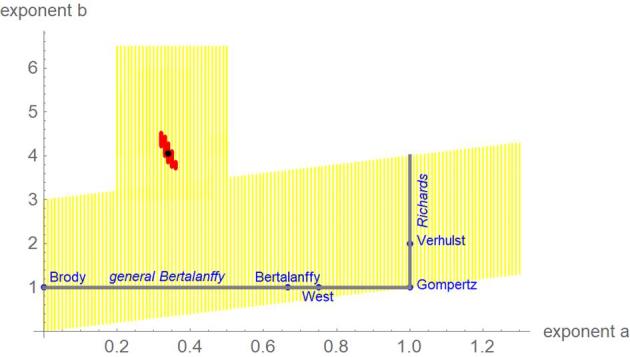
Exponent-pairs of the ‘named models’ (blue), the searched grid (yellow), the nearly optimal exponent-pairs (red), and the optimal exponent-pair (black), based on SSE.

Figure 2.

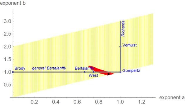
Exponent-pairs of the ‘named models’ (blue), the searched grid (yellow), the nearly optimal exponent-pairs (red) and the optimal exponent-pair (black), based on SSElog.

We considered the least squares fit SSE in order to compare our results with Aggrey (2002). The optimal exponent-pair was a = 0.34, b = 4.06 with SSE_opt = 2,214.799. This translated into a residual standard deviation RSD = 9.044. In comparison to the best-fit model of Aggrey (2002), this was a 31% improvement; Aggrey (2002) achieved the least RSD = 11.43 for the Gompertz model (a = b = 1). The other optimal parameters for the current model were m₀ = 17.131 g (compare to the average hatching mass of 37 g), p = 1.991 and q = 6.029 ⋅ 10⁻¹³. The asymptotic mass for the best-fitting growth curve was computed as 2,319.7 g (compare to the maximal observed mass: 2,267.7 g) and the mass at the inception point was 51.3% of the asymptotic mass. The maximal growth rate was 20.3 g/d (at the inflection point).

Assuming a log-normal distribution, the optimal exponent-pair was a = 0.89, b = 0.93 with SSE_opt = 0.0459878 and the optimal parameters m₀ = 32.92 g, p = 1.0952, and q = 0.799. The computed asymptotic mass was 2,671.1 g. The inflection point was attained at day 61; the mass at the inflection point was 33.3% of the asymptotic mass and the maximal weight gain was 19.9 g/day.

Figures 3 and 4 plot the mass-at-age data of the chicken and the optimal growth curves with the above parameters, using SSE and SSElog for comparison. Except for the curves for SSElog at the higher masses, there were barely visible differences between the optimal growth curves and the data. The visible differences for SSElog at the higher masses occurred for 2 reasons. First, younger animals were weighed more often (each third day; later only each second week), whence deviations at smaller weights were penalized more heavily. Second, under the lognormal distribution assumption the relative deviations matter and a deviation of a few percent is easier to discern for higher masses than for smaller ones.

Figure 3.

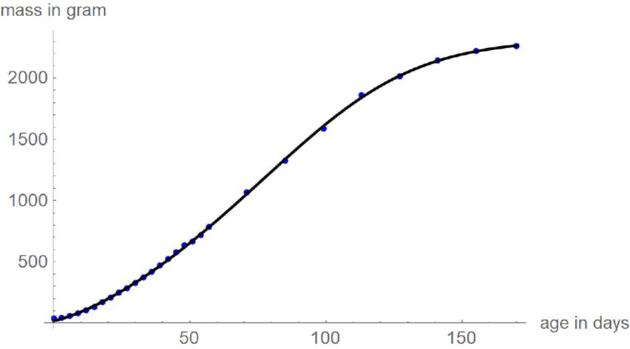
Data (blue) and optimal growth curve (black), based on SSE.

Figure 4.

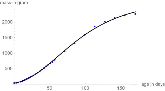
Data (blue) and optimal growth curve (black), based on SSElog.

Figures 5 to 8 exemplify the typical 4 phases of optimization for SSElog and they explain, how the method helped to verify the optimality of exponent-pairs. For small values of the exponent a (e.g., a = 0), there were large fluctuations in the computation of SSElog_opt, whence its value was not accurate. However, SSElog_opt was too large to be a candidate for the global minimum. This phase was followed by high values of SSElog_opt, whereby the minimum was attained for the maximal considered values of b (e.g., a = 0.5). However, owing to the flatness of this curve at b, it was not expected to find the overall optimal exponent-pairs for larger b. The third phase (e.g., a = 0.7) was characterized by the U-shape of SSElog_opt as a function of b. Here the minimum could be clearly discerned. At the final phase (e.g., a = 1.1), the optimum was achieved at the first grid point. Thereby, phases 3 and 4 appear to be typical for this optimization. For our data, the overall optimum of SSElog_opt was achieved in phase 3 and it increased for larger values of a. If the overall optimum were achieved in phase 4, then the optimization would have to be repeated for equation (2).

Figure 5.

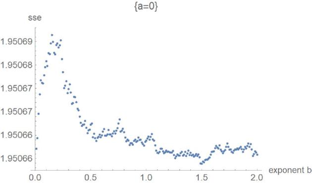
SSElog _opt(a, b) with fixed exponent a as a function of b for the first phase of optimization.

Figure 8.

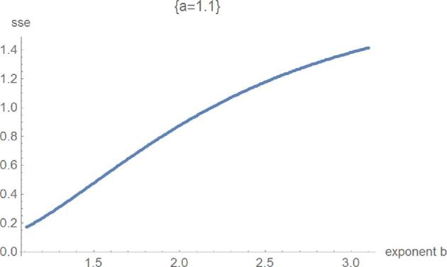
SSElog _opt(a, b) with fixed exponent a as a function of b for the fourth phase of optimization.

Figure 6.

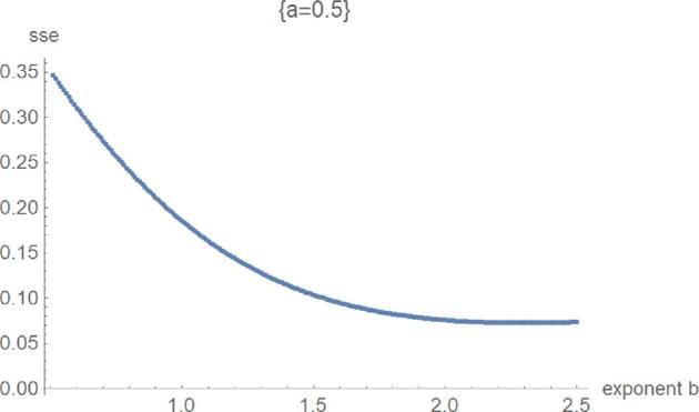
SSElog _opt(a, b) with fixed exponent a as a function of b for the second phase of optimization.

Figure 7.

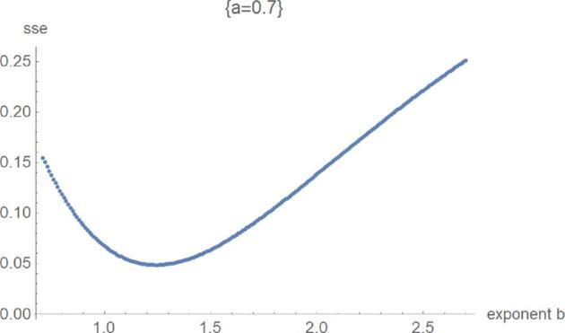
SSElog _opt(a, b) with fixed exponent a as a function of b for the third phase of optimization.

DISCUSSION

A biological analysis of growth requires an optimization of many potential models for many data about different species of chicken. For this purpose, the authors developed available method to identify the optimal exponent-pairs. It worked without human intervention and the reliability of the outcome could be judged from a study of the different phases of optimization. The application of this optimization method to different growth data and the biological interpretation of these results is a topic of future research. The paper served as a proof of principle using data for a well-established control strain of meat-type chicken, Athens Canadian Random Bred chicken (Collins et al., 2016).

The considered strain is a meat bird from 60 yr ago, which may no longer be representative of the modern broiler. We therefore propose a question for future research: What are the optimal exponents of modern strains, and if they differ from the old ones, into what direction did they move? Are there patterns that relate environmental factors and animal biology to the shape (e.g., size and location) of the regions of near-optimal exponent-pairs? How do the optimal exponent-pairs of individual chicken compare to those of their group?

However, there are possible drawbacks. For example, the optimal exponents and the regions of near-optimality did strongly depend on which method for data-fitting was used. We recommend using SSElog for optimization. First, it resulted in an exponent-pair that was close to the usual models. While the method of least squares (SSE) provided a visually excellent fit, the optimal exponents seem to contradict the intuitions of past researchers, who sought for optimal models with not so large exponents. Second, the assumption of a lognormal distribution, on which SSElog is based, was plausible for the used data, as the standard deviations were approximately proportional to mass. By contrast, the assumption of a normal distribution made SSE vulnerable to larger spreads for higher weights. Third, for the optimization using SSElog, a substantial speed-up is possible, as a smaller grid closer to the diagonal may be used. Thus, 1 to 2 D computation time per data are feasible, whence also the individual optimization for 100 to 200 chickens becomes feasible, if several computers are run in parallel. In comparison, optimization using SSE turned out to be impractical, as the large initial grid was too small; it finally was doubled.

As another possible drawback to the proposed research program, farmers change the feeding regime after 8 wk. Therefore, long-term data about growth under natural conditions need to be generated in laboratory studies. We checked, if 8 wk would be enough to study growth. Figure 9 illustrates that 8 wk would not suffice, as the prognosis of the model would be unreliable. However, using SSElog (but not SSE), 16 weeks may provide reasonable results.

Figure 9.

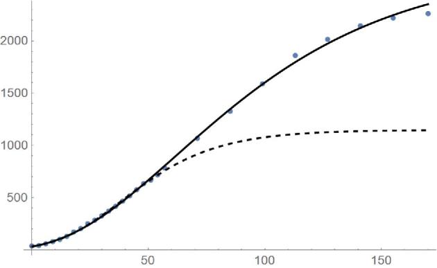
Data and best fit curves for the first 57and 131 D, based on SSElog.

REFERENCES

- Aggrey S. E. 2002. Comparison of three nonlinear and spline regression models for describing chicken growth curves. Poult. Sci. 81:1782–1788. [DOI] [PubMed] [Google Scholar]
- Bertalanffy L. v. 1957. Quantitative laws in metabolism and growth. Q. Rev. Biol. 32:217–231. [DOI] [PubMed] [Google Scholar]
- Brisbin I. L. Jr., Collins C. T., White G. C., McCallum D. A.. 1987. A new paradigm for the analysis and interpretation of growth data: the shape of things to come. The Auk 104:552–554. [Google Scholar]
- Brody S. 1945. Bioenergetics and Growth. Hafner Publ. Comp., New York, NY, USA. [Google Scholar]
- Burden R. L., Faires J. D.. 1993. Numerical Analysis. PWS Publ. Co., Boston, MA, USA. [Google Scholar]
- Collins K. E., Marks H. L., Aggrey S. E., Lacy M. P., Wilson J. L.. 2016. History of the Athens Canadian Random Bred and the Athens Random Bred control populations. Poult. Sci. 95:997–1004. [DOI] [PubMed] [Google Scholar]
- Gao C. Q., Yang J. X., Chen M. X., Yan H. C., Wang X. Q.. 2016. Growth curves and age-related changes in carcass characteristics, organs, serum parameters, and intestinal transporter gene expression in domestic pigeon (Columba livia). Poult. Sci. 95:867–877. [DOI] [PubMed] [Google Scholar]
- Gompertz B. 1832. On the nature of the function expressive of the law of human mortality, and on a new mode of determining the value of life contingencies. Philos. Trans. R. Soc. London 123:513–585. [DOI] [PMC free article] [PubMed] [Google Scholar]
- Gonçalves Gotuzzo Ariane, Piles Miriam, Della-Flora Raquel Pillon, Germano Jerusa Martins, Reis JanainaScaglioni, Tyska Darilene Ursula, LaurinoDionello Nelson José. 2018. Bayesian hierarchical model for comparison of different nonlinear function and genetic parameter estimates of meat quails. Poult. Sci. 10.3382/ps/pey548 [DOI] [PubMed] [Google Scholar]
- Grossman M., Bohren B. B., Anderson V. L.. 1985. Logistic growth curve of chickens: heritability of parameters. J. Hered. 76:459–462. [DOI] [PubMed] [Google Scholar]
- Isaac N. J. B., Carbone C.. 2010. Why are metabolic scaling exponents so controversial? Quantifying variance and testing hypotheses. Ecol. Lett. 13:728–735. [DOI] [PubMed] [Google Scholar]
- Kahm M., Hasenbrink G., Lichtenberg-Frate H., Ludwig J., Kschischo M.. 2010. Fitting biological growth curves with R. J. Stat. Softw. 33:1–21.20808728 [Google Scholar]
- Kuhi H. D., Porter T., López S., Kebreab E., Strathe A., Dumas A., France J.. 2010. A review of mathematical functions for the analysis of growth in poultry. Worlds Poult. Sci. J. 66:227–240. [Google Scholar]
- Leader J. J. 2004. Numerical Analysis and Scientific Computation. Addison-Wesley, Boston, USA. [Google Scholar]
- Manabe A., Yamakawa T., Ohnishi S., T., Akamine Y, Narimatsu, Tanaka H., T., Funamoto Y., Ueda, Yamamoto T.. 2018. A novel growth function incorporating the effects of reproductive energy allocation. PLoS One 13:e0199346. [DOI] [PMC free article] [PubMed] [Google Scholar]
- Marusic M., Bajzer Z.. 1993. Generalized two-parameter equations of growth. J. Math. Anal. Appl. 179:446–462. [Google Scholar]
- Ogle D., Iserman D. A.. 2017. Estimating age at a specified length from the von Bertalanffy growth function. N. Am. J. Fish. Manag. 37:1176–1180. [Google Scholar]
- Ohnishi S., Yamakawa T., Akamine T.. 2014. On the analytical solution for the Pütter-Bertalanffy growth equation. J. Theor. Biol. 343:174–177. [DOI] [PubMed] [Google Scholar]
- Pauly D. 1981. The relationship between gill surface area and growth performance in fish: a generalization of von Bertalanffy's theory of growth. Ber. Deutsch. Wiss. Kommiss. Meeresf. 28:25–282. [Google Scholar]
- Parks J. R. 1982. A Theory of Feeding and Growth of Animals. Springer Business Media, New York, USA. [Google Scholar]
- Pütter A. 1920. Studien über physiologische Ähnlichkeit VI. Wachstumsähnlichkeiten. Pflügers Arch. 180:298–340. [Google Scholar]
- Renner-Martin K., Kühleitner M., Brunner N., Hagmüller W.. 2016. AIC-based selection of growth models: the case of piglets from organic farming. OJMSi 4:17–23. [Google Scholar]
- Renner-Martin K., Brunner N., Kühleitner M., Nowak W. G., Scheicher K.. 2018. Optimal and near-optimal exponent-pairs for the Bertalanffy-Pütter growth model. PeerJ 6:e5973. [DOI] [PMC free article] [PubMed] [Google Scholar]
- Renner-Martin K., Brunner N., Kühleitner M., Nowak W. G., Scheicher K.. 2019. A model for the mass-growth of wild-caught fish. OJMSi 7:19–40. [Google Scholar]
- Richards F. J. 1959. A flexible growth function for empirical use. J. Exp. Bot. 10:290–301. [Google Scholar]
- Ricklefs R. E. 1967. A graphical method of fitting equations to growth curves. Ecology 48:978–983. [Google Scholar]
- Ricklefs R. E. 1968. Patterns of growth in birds. Ibis 110:419–451. [Google Scholar]
- Sariyel V., Aygun A., Keskin I.. 2017. Comparison of growth curve models in partridge. Poult. Sci. 96:1635–1640. [DOI] [PubMed] [Google Scholar]
- Shi P. J., Ishikawa T., Sandhu H. S., Hui C., Chakraborty A., Jin K. X. S., Tachihara, Li B. L.. 2014. On the 3/4-exponent von Bertalanffy equation for ontogenetic growth. Ecol. Modell. 276:23–28. [Google Scholar]
- Tompić T., Dobša J., Legen S., Tompić N., Medić H.. 2011. Modeling the growth pattern of in-season and off-season Ross 308 broiler breeder flocks. Poult. Sci. 90:2879–2887. [DOI] [PubMed] [Google Scholar]
- Verhulst P. F. 1838. Notice sur la loi que la population suit dans son accroissement. Curr. Math. Phys. 10:113–121. [Google Scholar]
- Vidal R. V. V. 1993. Applied Simulated Annealing. Lecture Notes in Economics and Mathematical Systems. Springer-Verlag, Berlin, Germany. [Google Scholar]
- West G. B., Brown J. H., Enquist B. J.. 2001. A general model for ontogenetic growth. Nature 413:628–631. [DOI] [PubMed] [Google Scholar]
- Wheldon T. E. 1988. Mathematical Models in Cancer Research. Adam Hilger; Bristol, UK. [Google Scholar]
Associated Data
This section collects any data citations, data availability statements, or supplementary materials included in this article.