Linear and Nonlinear Mixed-Effects Models for Censored HIV Viral Loads Using Normal/Independent Distributions

SUMMARY

HIV RNA viral load measures are often subjected to some upper and lower detection limits depending on the quantification assays. Hence, the responses are either left or right censored. Linear (and nonlinear) mixed-effects models (with modifications to accommodate censoring) are routinely used to analyze this type of data and are based on normality assumptions for the random terms. However, those analyses might not provide robust inference when the normality assumptions are questionable. In this article, we develop a Bayesian framework for censored linear (and nonlinear) models replacing the Gaussian assumptions for the random terms with normal/independent (NI) distributions. The NI is an attractive class of symmetric heavy-tailed densities that includes the normal, Student’s-t, slash, and the contaminated normal distributions as special cases. The marginal likelihood is tractable (using approximations for nonlinear models) and can be used to develop Bayesian case-deletion influence diagnostics based on the Kullback-Leibler divergence. The newly developed procedures are illustrated with two HIV AIDS studies on viral loads that were initially analyzed using normal (censored) mixed-effects models, as well as simulations.

1. Introduction

Studies of HIV viral dynamics, often considered to be the centerpiece of AIDS research, consider repeated/longitudinal measures over a period of treatment routinely analyzed using linear and nonlinear mixed-effects models (LME/NLME) to assess rates of changes in HIV-1 RNA level or viral load (H. Wu, 2005; L. Wu, 2010). Viral load measures the amount of actively replicating virus and its reduction is frequently used as a primary endpoint in clinical trials of antiretroviral therapy. However, depending upon the diagnostic assays used, its measurement may be subjected to some upper and lower detection limits (hence, left or right censored), below or above which they are not quantifiable. The proportion of censored data in these studies may not be trivial (Hughes, 1999) and considering crude/ad hoc methods, namely, substituting threshold value or some arbitrary point such as midpoint between zero and cutoff for detection (Vaida and Liu, 2009) might lead to biased estimates of fixed effects and variance components (L. Wu, 2010).

Our motivating datasets in this study are on HIV-1 viral load, (i) after unstructured treatment interruption, or UTI (Saitoh et al., 2008) and (ii) set point for acutely infected subjects from the Acute Infection and Early Disease Research Program (AIEDRP) program (Vaida and Liu, 2009). The former has about 7% observations below (left censored) the detection limits, whereas the latter has about 22% lying above (right censored) the limits of assay quantifications. As alternatives to crude imputation methods, Hughes (1999) proposed a likelihood-based Monte Carlo expectation-maximization (EM) algorithm (MCEM) for LME with censored responses (LMEC). Vaida, Fitzgerald, and DeGrut-tola (2007) proposed a hybrid EM using a more efficient Hughes’ algorithm, extending it to NLME with censored data (NLMEC). Recently, Vaida and Liu (2009) proposed an exact EM algorithm for LMEC/NLMEC, which uses closed-form expressions at the E-step, as opposed to Monte Carlo simulations. A common feature of all these methods is the fidelity to the “Gaussian” paradigm for the random effects and within-subject random errors. Even though normality may be a reasonable model assumption, it may lack robustness in parameter estimation under departures from normality (namely, heavy tails) and/or outliers (Pinheiro, Liu, and Wu, 2001). Viral load measurements are often skewed with heavy right (or left) tail, and even log transformations on the responses do not render normality. These characteristics further complicate analysis of mixed-effects models, because both the (within-subject) random error and (between-subject) random effects might contribute to the “shift from normality.” For example, Figure 1 (panels a and b) displays density histogram and Q-Q plots of empirical Bayes’ estimates of random effects, respectively, obtained by fitting a classical LMEC model using R package lmec to the UTI data. The plots reveal subject-specific intercepts behaving somewhat symmetrically, with evident outliers (b-outliers) at the level of the random effects as well as at the within-subject levels (e-outliers), demonstrated through the residual Q-Q plot in Figure 1 (panel c).

Figure 1.

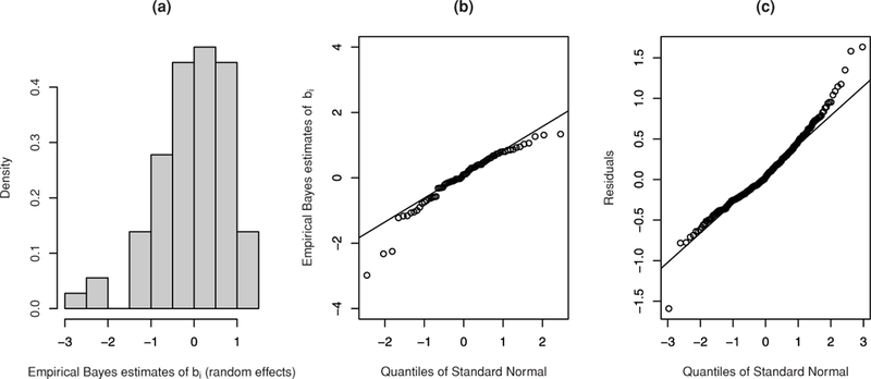
Plots of density histogram (panel a) and normal Q-Q plot (panel b) of empirical Bayes’ estimates of random effects obtained by fitting LMEC to the UTI data. Panel (c) displays normal Q-Q plot for model residuals.

In presence of longer-than-normal tails/outliers, popular data transformations (namely, Box-Cox, etc.) might render normality, or close to normality with reasonable empirical results; however, (i) transformation provides reduced information on an underlying data generation scheme, (ii) component-wise transformation might not guarantee joint normality, (iii) parameters might lose interpretability on a transformed scale, and (iv) transformations may not be universal and usually vary with the dataset. Hence from a practical perspective, there is a necessity to seek an appropriate theoretical model that avoids data transformations, yet presents a ro-bustified “Gaussian” framework. For complete data, some proposals replace normality with more flexible classes of distributions, namely, a t-linear mixed model (T-LME) (Pin-heiro et al., 2001; Lin and Lee, 2006, 2007). From a Bayesian perspective, Liu (1996) discussed a class of robust distributions, called normal/independent (NI) distributions (Lange and Sinsheimer, 1993) for multivariate linear regression models and Rosa, Padovani, and Gianola (2003) extended it for heavy-tailed LME (NI-LME). Although some results on LME/NLME with elliptical distributions have recently appeared in the literature (Russo, Paula, and Aoki, 2009), to the best of our knowledge, there seem to be no studies on Bayesian inference for NLMEC/LMEC using the NI class. Here, we propose a robust Bayesian parametric framework for NLMEC/LMEC and related Kullback-Leibler (K-L) influence diagnostics (Peng and Dey, 1995) based on the NI class and apply it to two motivating HIV datasets. The term “robustness” is quite extensive, here it is achieved in terms of Bayesian parameter estimation. The theoretical justification rests on the facts that the NI class stochastically attributes varying weights to each subject, i.e., lower weight for outliers (see Web Figure 1) and thus controls the influence of subject-level data on the overall inference. Also, every member of the NI class tends to the normal case, for example, as the t degrees of freedom → ∞ to, it approaches normality.

The rest of the article proceeds as follows. In Section 2, after a brief introduction of NI distributions, we propose the NI-LMEC and related Bayesian inference. Section 3 deals with Bayesian inference for NI-NLMEC. Section 4 presents Bayesian model selection tools and related case influence diagnostics. The advantage of the proposed methodology is illustrated through the two motivating AIDS datasets in Section 5. Section 6 presents a simulation study to compare the performance of our proposed methods with other “normality”-based methods. Section 7 concludes with some discussions and possible directions for future research.

2. Linear Mixed-Effects Models with Censored Responses

2.1. Normal/Independent Distributions

We start with some background on the class of NI distributions as proposed in Lange and Sinsheimer (1993). An element of the NI family is defined as the distribution of the p-variate random vector $\mathbf{y}=\mathit{\mu }+U^{-1/2}\mathbf{Z}$, where μ is a location vector, Z is a normal random vector with mean vector 0, variance-covariance matrix Σ and U is a mixing positive random variable with cumulative distribution function H (u | ν) and probability density function (pdf) H(u | ν), independent of Z, where ν is a scalar or parameter vector indexing the distribution of U. Note that given U, y follows a multivariate normal distribution with mean vector μ and variance-covariance matrix u⁻¹Σ with the pdf of y given by $\text{NI}(\mathbf{y}|\mathit{\mu },\mathbf{\Sigma },\mathit{\nu })={\int }_0^{\infty }{\varphi }_p\left(\mathbf{y};\mathit{\mu },u^{-1}\mathbf{\Sigma }\right)dH(u|\mathit{\nu })$, where ${\varphi }_p(.;\mathit{\mu },\mathbf{\Sigma })$ stands for the pdf of the p-variate normal distribution with mean vector μ and covariate matrix Σ. We shall use the notation NI_p (μ, Σ, H) to indicate that y is a distribution in the NI class. When H is degenerate (U = 1), NI_p (μ, Σ, H) is normally distributed. The NI family constitutes a class of thick-tailed distributions, some of which are the multivariate versions of the Student’s-t, slash, and the contaminated normal (CN) distributions (see Web Appendix A for more details).

2.2. Model Specification

Ignoring censoring for the moment, we proceed as in Pinheiro et al. (2001) and Lin and Lee (2006) by considering a generalization of the classical normal LME as follows:

$${\mathbf{y}}_i={\mathbf{X}}_i\mathit{\beta }+{\mathbf{Z}}_i{\mathbf{b}}_i+{\mathit{ϵ}}_i,i=1,\dots ,n,\text{with}$$ (1)

$${\left({\mathbf{b}}_i,{\mathit{ϵ}}_i\right)}^{\top }~N{I}_{n_i+q}\left\{\mathbf{0},\mathrm{Diag}\left(\mathbf{\Sigma },{\sigma }^2{\mathbf{I}}_{n_i}\right),H\right\},$$ (2)

where subscript i is the subject index; I_p denotes the p × p identity matrix; Diag(A, B) denotes a block diagonal matrix whose elements are the square matrices A and B; ${\mathbf{y}}_i={\left(y_{i1},\dots ,y_{i{n}_i}\right)}^{\top }$ is a n_i × 1 vector of observed continuous responses for subject i, X_i and Z_i are known full-rank design matrices of dimensions n_i × p and n_i × q, respectively; β is a p × 1 vector of population-level fixed effects; b_i is a q × 1 vector of unobservable random effects; ϵ_i is the n_i × 1 vector of random errors; and the dispersion matrix D = D (α) depends on unknown and reduced parameter vector α. Using the definition of a NI random vector and (2), it follows that marginally

$$\begin{array}{l}{\mathbf{b}}_i\stackrel{i.i.d.}{~}N{I}_q(\mathbf{0},\mathbf{D},H)\text{and}{\mathit{ϵ}}_i\stackrel{\mathit{\text{ind}}.}{~}N{I}_{n_i}\left(\mathbf{0},{\sigma }^2{\mathbf{I}}_{n_i},H\right),\\ i=1,\dots ,n.\end{array}$$ (3)

Conditional on U_i, b_i and ϵ_i are independent, as well as uncorrelated because $\text{Cov}\left({\mathbf{b}}_i,{\mathit{ϵ}}_i\right)=E\left({\mathbf{b}}_i{\mathit{ϵ}}_i^{\top }\right)=E\left\{E\left({\mathbf{b}}_i{\mathit{ϵ}}_i^{\top }|U_i\right)\right\}=\mathbf{0}$. In the present formulation, we consider the case where the response Y_ij is not fully observed for all i, j. Let the observed data for the ith subject be (Q_i, C_i), where Q_i represents the vector of uncensored reading or censoring level, and C_i the vector of censoring indicators, such that

$$y_{ij}⩽Q_{ij}\text{if}{C}_{ij}=1,\text{and}{y}_{ij}=Q_{ij}\text{if}{C}_{ij}=0.$$ (4)

For simplicity, we will assume that the data are left censored. The extensions to arbitrary censoring are immediate. Following Vaida and Liu (2009), classical inference on the parameter vector $\mathit{\theta }={\left({\mathit{\beta }}^{\top },{\sigma }^2,{\mathit{\alpha }}^{\top },{\mathit{\nu }}^{\top }\right)}^{\top }$ is based on the marginal distribution of y_i. For complete data, we have that marginally ${\mathbf{y}}_i\stackrel{\text{ind.}}{~}N{I}_{n_i}\left({\mathbf{X}}_i\mathit{\beta },{\mathbf{\Sigma }}_i,H\right)$ where ${\mathbf{\Sigma }}_i={\sigma }^2{\mathbf{I}}_{ni}+{\mathbf{Z}}_i\mathbf{D}{\mathbf{Z}}_i^{\top }$. For responses with censoring pattern as in (4), we have that ${\mathbf{y}}_i~TN{I}_{n_i}\left({\mathbf{X}}_i\mathit{\beta },{\mathbf{\Sigma }}_i,H;\mathbb{A}\right)$, where $TN{I}_{n_i}(.;\mathbb{A})$ denotes the truncated NI distribution on the interval $\mathbb{A}$, where ${\mathbb{A}}_i=A_{i1}\times \dots ,\times A_{ini}$, with A_ij as the interval (−∞, ∞), if C_ij = 0 and (−∞, Q_ij], if C_ij = 1. Specifically, a p-dimensional vector $\mathbf{X}~TN{I}_p(\mathit{\mu },\mathbf{\Sigma },\mathit{\nu };\mathbb{A})$ if its density is given by $TN{I}_p(\mathbf{x}|\mathit{\mu },\mathbf{\Sigma },\mathit{\nu };\mathbb{A})=\frac{N{I}_p(\mathbf{x}|\mathit{\mu },\mathbf{\Sigma },\mathit{\nu })}{{\prod }_{r=1}^p{\int }_{-\infty }^{a_r}N{I}_p(\mathbf{x}|\mathit{\mu },\mathbf{\Sigma },\mathit{\nu })d\mathbf{x}}{\mathbb{I}}_{(\mathbb{A})}(\mathbf{X})$, where the notation ${\prod }_{r=1}^p{\int }_{-\infty }^{a_r}={\int }_{-\infty }^{a_1}\dots {\int }_{-\infty }^{a_p}$ stand for the abbreviation of multiple integrals. For computing the likelihood function, the first step is to treat separately the observed and censored components of y_i. Let ${\mathbf{y}}_i^o$ be the $n_i^o$-vector of observed outcomes and ${\mathbf{y}}_i^c$ be the $n_i^c$-vector of censored observations for subject i with $\left(n_i=n_i^o+n_i^c\right)$, such that, C_ij = 0 for all elements in ${\mathbf{\text{y}}}_i^o$, and 1 for all elements in ${\mathbf{\text{y}}}_i^c$. After reordering, y_i, Q_i, X_i, and Σ_i can be partitioned as follows: ${\mathbf{y}}_i=\mathrm{vec}\left({\mathbf{y}}_i^o,{\mathbf{y}}_i^c\right)$, ${\mathbf{Q}}_i=\mathrm{vec}\left({\mathbf{Q}}_i^o,{\mathbf{Q}}_i^c\right)$, ${\mathbf{X}}_i^{\top }=\left({\mathbf{X}}_i^o,{\mathbf{X}}_i^c\right)$ and ${\mathbf{\Sigma }}_i=\left(\begin{array}{cc}{\mathbf{\Sigma }}_i^{oo}& {\mathbf{\Sigma }}_i^{oc}\\ {\mathbf{\Sigma }}_i^{co}& {\mathbf{\Sigma }}_i^{cc}\end{array}\right)$, where vec(.) denote the function which stacks vectors or matrices of the same number of columns. Then we have ${\mathbf{y}}_i^o~N{I}_{n_i^o}\left({\mathbf{X}}_i^o\mathit{\beta },{\mathbf{\Sigma }}_i^{oo},H\right)$, ${\mathbf{y}}_i^c|{\mathbf{y}}_i^o,u_i~N_{n_i^c}\left({\mathit{\mu }}_i,u_i^{-1}{\mathbf{S}}_i\right)$, where ${\mathit{\mu }}_i={\mathbf{X}}_i^c\mathit{\beta }+{\mathbf{\Sigma }}_i^{co}{\left({\mathbf{\Sigma }}_i^{oo}\right)}^{-1}({\mathbf{y}}_i^o-{\mathbf{X}}_i^o\mathit{\beta })$ and ${\mathbf{S}}_i={\mathbf{\Sigma }}_i^{cc}-{\mathbf{\Sigma }}_i^{co}{\left({\mathbf{\Sigma }}_i^{oo}\right)}^{-1}{\mathbf{\Sigma }}_i^{oc}$. Now, let ${\mathbf{\text{Φ}}}_{n_i}(\mathbf{u};\mathbf{a},\mathbf{A})$ and ${\varphi }_{n_i}(\mathbf{u};\mathbf{a},\mathbf{A})$ be the cumulative distribution function (left tail) and pdf, respectively, of $N_{n_i}(\mathbf{a},\mathbf{A})$ computed at u. From Vaida and Liu (2009) and Jacqmin-Gadda et al. (2000), the likelihood function for cluster i (using conditional probability arguments) is given by

$$\begin{gathered} L_i(\mathit{\theta })=f\left({\mathbf{y}}_i^o|\mathit{\theta }\right)P\left({\mathbf{y}}_i^c⩽{\mathbf{Q}}_i^c|{\mathbf{y}}_i^o,\mathit{\theta }\right) \\ ={\int }_0^{\infty }{\varphi }_{n_i}\left({\mathbf{y}}_i^o;{\mathbf{X}}_i^o\mathbf{\beta },u^{-1}{\mathbf{\Sigma }}_i^{oo}\right){\mathbf{\text{Φ}}}_{n_i^c}\left({\mathbf{Q}}_i^c;{\mathbf{\mu }}_i,u^{-1}{\mathbf{S}}_i\right)dH(u), \end{gathered}$$

and the full likelihood given by $\mathcal{l}(\mathit{\theta }|\mathbf{y})={\sum }_{i=1}^n\left\{\log L_i(\mathit{\theta })\right\}$, which would yield maximum likelihood (ML) inference through EM-type algorithms. Our proposition uses the Bayesian paradigm for a number of reasons, primarily motivated by the computational simplicity achieved. Although both the EM-type algorithms and full Bayes’ approach uses “often identical” Gibbs steps, the M-step in the EM routine for complicated LMEC/NLMEC models is computationally cumbersome, and hence a single run of the EM routine is often more time consuming (Liu et al., 2010) than the Bayesian updating, assuming equal number of Gibbs iterations. The high-dimensional integrals in our likelihood function further complicates ML-type estimation (involving multiparameter variance estimation through observed Fisher information inversion), except under normality and linearity assumptions. Often, asymptotic theory of maximum likelihood estimation (MLE) may not be applicable for moderate-size censored data, and it is often difficult to develop or justify the theoretical properties of these classical approaches. On the contrary, recent developments in Markov chain Monte Carlo (MCMC) methods facilitate easy and straightforward implementation of the Bayesian paradigm through conventional software such as WinBUGS. The Bayesian approach allows extreme flexibility in fitting realistic models to datasets of varying complexity (Dunson, 2001), makes use of all information available in the relevant clinical study/trial, accommodates full parameter uncertainty through appropriate prior choices supported with proper sensitivity investigations, provides direct probability statement about a parameter through credible intervals (CI), and does not depend on asymptotic results.

2.3. Prior and Posterior Specifications

To complete the Bayesian specification, we need to consider prior distributions for all the unknown model parameters $\mathit{\theta }={\left({\mathit{\beta }}^{\top },{\sigma }^2,{\mathit{\alpha }}^{\top },\mathit{\nu }\right)}^{\top }$. A popular choice to ensure posterior propriety in a linear mixed model (LMM) is to consider proper (but diffuse) conditionally conjugate priors (Hobert and Casella, 1996). Thus, we have $\mathit{\beta }~N_p\left({\mathit{\beta }}_0,{\mathbf{S}}_{\beta }\right)$, ${\sigma }^2~IGamma\left(q_0/2,{\lambda }_0/2\right)$, and $\mathbf{D}~IWis{h}_q\left({\mathbf{\Lambda }}_0^{-1},{\nu }_0\right)$, where IGamma(a, b) is the inverse gamma distribution with mean b/(a − 1), a > 1, and IWish_q(M⁻¹, ν₀) is the inverse Wishart distribution with mean M⁻¹/(ν₀ − q − 1), {ν₀ > q + 1, where M is a q × q known positive definite matrix. For the specific models in Subsection 2.1, the prior for ν was chosen accordingly as follows.

1. Student’s-t model: Here $\nu ~TExp\left\{\frac{\gamma }{2};(2,\infty )\right\}$, i.e., the degrees of freedom parameter ν has a truncated exponential prior distribution on the interval (2, ∞). This truncation point was chosen to assure finite variance.

2. Slash model: A Gamma (a, b) distribution with small positive values of a and $b(b\ll a)$ is adopted as a prior distribution for ν.

3. Contaminated normal model: A Beta (ν₀, ν₁) distribution is used as a prior for ν, and an independent Beta (ρ₀, ρ₁) is adopted as prior for ρ.

Henceforth (unless otherwise stated), $f(\cdot )$ denotes densities, whereas the arguments in parentheses represent associated random variables. Assuming elements of the parameter vector to be independent, our Bayesian model allows straightforward construction of a Gibbs sampler. Denote $\mathbf{\text{y}}={\left({\mathbf{y}}_1^{\top },\dots ,{\mathbf{y}}_n^{\top }\right)}^{\top }$, $\mathbf{b}={\left({\mathbf{b}}_1^{\top },\dots ,{\mathbf{b}}_n^{\top }\right)}^{\top }$ and $\mathbf{u}={\left(u_1,\dots ,u_n\right)}^{\top }$, $\mathbf{\text{Q}}=\mathrm{vec}\left({\mathbf{\text{Q}}}_1,\dots ,{\mathbf{\text{Q}}}_n\right)$ and $\mathbf{\text{C}}=\mathrm{vec}\left({\mathbf{\text{C}}}_1,\dots ,{\mathbf{\text{C}}}_n\right)$. Given u, all conditional posterior distributions are as in a standard N-LMEC model and have the same form for any element of the NI family. These are given by

1. y_i | b_i, u_i, C_i, Q_i, θ ~ f(y_i | b_i, u_i, C_i, Q_i, θ). Thus, conditional on (b_i, u_i), y_i is a vector of independent observations distributed as truncated normal, each with untruncated variance $u_i^{-1}{\sigma }^2$ and untruncated mean ${\mathbf{x}}_{ij}^{\top }\mathit{\beta }+{\mathbf{z}}_{ij}^{\top }$ b_i on the interval $y_{ij}⩽Q_{ij}$. We will use the notation $TN\left\{{\mathbf{x}}_{ij}^{\top }\mathit{\beta }+{\mathbf{z}}_{ij}^{\top }{\mathbf{b}}_i,u_i^{-1}{\sigma }^2;\left(-\infty ,Q_{ij}\right)\right\}$ in this context.

2. b_i | y_i, u_i, C_i, Q_i, θ = b_i | y_i, u_i, θ ~ f(b_i | y_i, u_i, θ). This distribution is multivariate normal with mean ${\widehat{\mathbf{b}}}_i={\mathbf{\Lambda }}_i{\mathbf{Z}}_i^{\top }\left({\mathbf{y}}_i-{\mathbf{X}}_i\mathit{\beta }\right)$ and variance $u_i^{-1}{\mathbf{\Lambda }}_i$, with ${\mathbf{\Lambda }}_i={\left({\mathbf{D}}^{-1}+{\sigma }^2{\mathbf{Z}}_i^{\top }{\mathbf{Z}}_i\right)}^{-1}$. Note that the entire vector y_i is used for sampling from b_i.

3. Because θ₁ | y, C, Q, ${\mathit{\theta }}_{\left(-{\mathit{\theta }}_1\right)}$ and ${\mathit{\theta }}_1|\mathbf{y},{\mathit{\theta }}_{\left(-{\mathit{\theta }}_1\right)}$ are two equivalent processes, we have:

   $$\begin{gathered} \mathit{\beta }|\mathbf{y},\mathbf{b},\mathbf{u},{\mathit{\theta }}_{(-\mathit{\beta })}~N\left({\mathbf{A}}_{\beta }{\mathit{\mu }}_{\beta },{\mathbf{A}}_{\beta }\right),{\sigma }^2|\mathbf{y},\mathbf{b},\mathbf{u},{\mathit{\theta }}_{\left(-{\sigma }^2\right)} \\ ~IGamma\left(\frac{q_0+N}{2},\frac{{\lambda }_0+s}{2}\right), \end{gathered}$$

   $$\mathbf{D}|\mathbf{y},\mathbf{b},\mathbf{u},{\mathbf{\theta }}_{(-\mathbf{\alpha })}~IWis{h}_q\left({\mathbf{\Lambda }}^{-1},{\nu }_0+n\right),$$

   where ${\mathbf{\mu }}_{\beta }=\left\{{\mathbf{S}}_{\beta }^{-1}{\mathbf{\beta }}_0+{\sum }_{i=1}^n{u}_i{\mathbf{X}}_i^{\top }\left({\mathbf{y}}_i-{\mathbf{Z}}_i{\mathbf{b}}_i\right)\right\}$, ${\mathbf{A}}_{\beta }=({\mathbf{S}}_{\beta }^{-1}+{\sum }_{i=1}^n{u}_i{\mathbf{X}}_i^{\top }{\mathbf{X}}_i{)}^{-1}$, $N={\sum }_{i=1}^n{n}_i$, $s={\sum }_{i=1}^n{u}_i{\lambda }_{1i}$, $\mathbf{\Lambda }={\mathbf{\Lambda }}_0+{\sum }_{i=1}^n{u}_i{\mathbf{b}}_i{\mathbf{b}}_i^{\top }$, with ${\lambda }_{1i}=({\mathbf{y}}_i-{\mathbf{X}}_i\mathit{\beta }-{\mathbf{Z}}_i{\mathbf{b}}_i{)}^{\top }$ $({\mathbf{y}}_i-{\mathbf{X}}_i\mathit{\beta }-{\mathbf{Z}}_i{\mathbf{b}}_i)$.

4. To complete the Gibbs sampling specifications, we need the full conditional posterior distributions of u and parameter ν, which depends on the density $h(.|\mathit{\nu })$. The general form for u_i is $\pi \left(u_i|\mathbf{y},\mathbf{b},\mathit{\theta }\right)\propto u_i^{\left(n_i+q\right)/2}h\left(u_i|\mathit{\nu }\right)\exp \left\{-\frac{u_i}{2}\left(\frac{{\lambda }_{1i}}{{\sigma }_i^2}+{\mathbf{b}}_i^{\top }{\mathbf{D}}^{-1}{\mathbf{b}}_i\right)\right\}$. For ν, the density is $\pi \left\{\mathit{\nu }|\mathbf{y},\mathbf{b},\mathbf{u},{\mathit{\theta }}_{(-\nu )}\right\}\propto \pi (\mathit{\nu }){\prod }_{i=1}^{n}h\left(u_i|\mathit{\nu }\right)$. The form of u_i and ν depends on the specific NI distribution adopted and also on the prior for ν (see Web Appendix A).

3. Nonlinear Mixed-Effects Models with Censored Responses

3.1. Model Specification

Extending the notation of the previous section and ignoring censoring, we first propose the following general mixed-effects model in which the random terms are assumed to follow a NI distribution (NI-NLME). Let ${\mathbf{y}}_i={\left(y_{i1},\dots ,y_{i{n}_i}\right)}^{\top }$ denote the (continuous) response vector for subject i and $\eta ={\left\{\eta \left({\mathbf{X}}_{i1},{\varphi }_i\right),\dots ,\eta \left({\mathbf{X}}_{i{n}_i},{\varphi }_i\right)\right\}}^{\top }$ be a nonlinear vector-valued differentiable function of the random parameter ϕ_i and co-variate vector X_i. The NI-NLME can then be expressed as:

$${\mathbf{y}}_i=\eta \left({\varphi }_i,{\mathbf{X}}_i\right)+{\mathit{ϵ}}_i,{\varphi }_i={\mathbf{A}}_i\mathit{\beta }+{\mathbf{B}}_i{\mathbf{b}}_i,$$ (5)

where A_i and B_i are known design matrices of dimensions r × p and r × q, respectively (possibly depending on some covariate values), β is the p × 1 vector of fixed effects, and B_i, is the q × 1 vector of random effects. The joint distribution of (b_i, ϵ_i) follows (2). From the definition of NI distributions and (2), we have that marginally ${\varphi }_i\stackrel{ind}{~}N{I}_q\left({\mathbf{A}}_i\mathit{\beta },{\mathbf{B}}_i\mathbf{D}{\mathbf{B}}_i^{\top },H\right)$ and ${\mathit{ϵ}}_i\stackrel{in\mathrm{d.}}{~}N{I}_{n_i}\left(\mathbf{0},{\sigma }^2{\mathbf{I}}_{n_i},H\right)$, and as in the linear case, they are uncorrelated because $\text{Cov}\left({\varphi }_i,{\mathit{ϵ}}_i\right)=\mathbf{0}$. For NI-NLME with complete responses, the marginal distribution is given by

$$\begin{gathered} f(\mathbf{y}|\mathbf{\theta })=\prod _{i=1}^n{\int }_0^{\infty }{\int }_{{ℝ}^q}{\varphi }_{n_i}\left\{{\mathbf{y}}_i;\eta \left({\varphi }_i,{\mathbf{X}}_i\right),u_i^{-1}{\sigma }^2{\mathbf{I}}_{n_i}\right\}{\varphi }_q \\ \times \left({\varphi }_i;{\mathbf{A}}_i\mathit{\beta },u_i^{-1}{\mathbf{B}}_i\mathbf{D}{\mathbf{B}}_i^{\top }\right)d{\varphi }_{i}dH\left(u_i|\mathit{\nu }\right), \end{gathered}$$

which generally does not have a closed-form expression because the model is not linear in random effects. In the normal case, various approximations (namely, first-order Taylor series expansion of the model function around the conditional mode of b_i) have been proposed to achieve tractable numerical optimizations (Lindstrom and Bates, 1990). Most algorithms for computing the approximate MLE $\widehat{\mathit{\theta }}$ and empirical Bayes’ estimators (predictors) for the random effects ${\widehat{\mathbf{b}}}_i$ consider iterative maximization of the approximate log-likelihood functions $\mathcal{l}(\mathbf{\theta },\tilde{\mathbf{b}})=\sum _{i=1}^n\log f\left({\mathbf{y}}_i|\mathit{\theta },{\tilde{\mathbf{b}}}_i\right)$. Following Taylor series expansions, we have the following theorem, whose proof is given in the Web Appendix B.

THEOREM 1.

Let $\tilde{\mathbf{b}}$ be an expansion point in a neighborhood of b_i, then under the NI-NLME model as in (5), the marginal distribution of y_i, can be approximated as ${\mathbf{y}}_i~N{I}_{ni}\left\{\eta \left({\mathbf{A}}_i\mathit{\beta }+{\mathbf{B}}_i{\tilde{\mathbf{b}}}_i,{\mathbf{X}}_i\right)-{\mathbf{H}}_i{\tilde{\mathbf{b}}}_i,{\tilde{\mathbf{V}}}_i,H\right\}$, where ${\tilde{\mathbf{V}}}_i=\left({\tilde{\mathbf{H}}}_i{\mathbf{B}}_i\right)\mathbf{D}{\left({\tilde{\mathbf{H}}}_i{\mathbf{B}}_i\right)}^{\top }+{\sigma }^2{\mathbf{I}}_{n_i}$, ${\tilde{\mathbf{H}}}_i={\frac{\partial \eta \left({\mathbf{A}}_i\mathit{\beta }+{\mathbf{B}}_i{\mathbf{b}}_i,{\mathbf{X}}_i\right)}{\partial {\mathbf{b}}_i^{\top }}|}_{{\mathbf{b}}_i={\tilde{\mathbf{b}}}_i}$ and $\dot{~}$ denotes approximated in distribution.

Our empirical Bayes’ estimates of the random effects ${\tilde{\mathbf{b}}}^{(k)}$ can be approximated as ${\tilde{\mathbf{b}}}_i^{(k)}=\text{E}\left\{{\mathbf{b}}_i|{\mathbf{y}}_i,{\widehat{\mathit{\theta }}}^{(k-1)}\right\}\approx {\widehat{\mathbf{\Lambda }}}_i^{(k-1)}{\tilde{\mathbf{H}}}_i^{(k-1)}\left\{{\mathbf{y}}_i-\eta \left({\mathbf{A}}_i{\widehat{\mathit{\beta }}}^{(k-1)}+{\mathbf{B}}_i{\tilde{\mathbf{b}}}_i^{(k-1)},{\mathbf{X}}_i\right)+{\tilde{\mathbf{H}}}_i^{(k-1)}{\tilde{\mathbf{b}}}_i^{(k-1)}\right\}$, where ${\widehat{\mathbf{\Lambda }}}_i^{(k-1)}={\left\{{\widehat{\mathbf{D}}}^{-1(k-1)}+\frac{1}{{\widehat{\sigma }}_e^{2(k-1)}}{\tilde{\mathbf{H}}}_i^{(k-1)\top }{\tilde{\mathbf{H}}}_i^{(k-1)}\right\}}^{-1}$. Note that the distribution of b_i | y_i is approximately symmetric (see Web Appendix B), and thus ${\tilde{\mathbf{b}}}_i^{(k)}$ is the mode of the distribution at each step. We have used this strategy to calculate the likelihood function and hence compute various Bayesian model selection/diagnostics. Now assuming left censoring such that the observed data for the ith subject be (Q_i, C_i), the individual observations within cluster i follows (4), so that the NI-NLMEC is defined. From Theorem 1, the approximated log-likelihood function for NI-NLMEC is a LMEC model with the same structure as indicated in (1), (2), and (4) and can be computed as described in Subsection 2.2. In the next subsection, we present full conditionals for the NI-NLMEC model parameters.

3.2. Prior and Posterior Specifications

Under the same prior specifications as discussed in Subsection 2.3, the full conditional distributions for NI-NLMEC models are as follows:

$$y_{ij}|{\varphi }_i,u_i,{\mathbf{C}}_i,{\mathbf{Q}}_i,\mathit{\theta }~TN\left\{\eta \left({\varphi }_i,{\mathbf{X}}_{ij}\right),u_i^{-1}{\sigma }^2;\left(-\infty ,Q_{ij}\right)\right\};$$

$${\varphi }_i|{\mathbf{y}}_i,u_i,\mathit{\theta }\propto {\varphi }_{n_i}\left\{{\mathbf{y}}_i;\eta \left({\varphi }_i,{\mathbf{X}}_i\right),u_i^{-1}{\sigma }^2{\mathbf{I}}_{n_i}\right\}{\varphi }_q\left({\varphi }_i;{\mathbf{A}}_i\mathit{\beta },u_i^{-1}{\mathbf{B}}_i\mathbf{D}{\mathbf{B}}_i^{\top }\right);$$

$$\mathit{\beta }|\mathbf{y},\varphi ,\mathbf{u},{\mathit{\theta }}_{(-\beta )}~N_p\left({\mathbf{A}}_{\beta }{\mathit{\mu }}_{\beta },{\mathbf{A}}_{\beta }\right);{\sigma }^2|\mathbf{y},\varphi ,\mathbf{u},{\mathit{\theta }}_{\left(-{\sigma }^2\right)}~IGamma\left(\frac{N+q_0}{2},\frac{{\lambda }_0+s}{2}\right);$$

$$\mathbf{D}|\mathbf{y},\varphi ,\mathbf{u},{\mathit{\theta }}_{(-\mathit{\alpha })}~{\mathit{IWish}}_q({\mathbf{\Lambda }}^{-1},{\mathit{\nu }}_0+n);\pi \{\mathit{\nu }|\mathbf{y},\mathit{\varphi },\mathbf{u},{\mathit{\theta }}_{\left(-\mathit{\nu }\right)}\left\}\propto \pi \right(\mathit{\nu }){\prod }_{i=1}^{n}h(u_i|\mathit{\nu });$$

$$\pi \left(u_i|{\mathbf{y}}_i,{\varphi }_i,\mathit{\theta }\right)\propto u_i^{\left(n_i+q\right)/2}h\left(u_i|\mathit{\nu }\right)\exp \left[-\frac{u_i}{2}\left\{\frac{{\lambda }_{1i}}{{\sigma }^2}+{\left({\varphi }_i-{\mathbf{A}}_i\mathit{\beta }\right)}^{\top }{\left({\mathbf{B}}_i\mathbf{D}{\mathbf{B}}_i^{\top }\right)}^{-1}\left({\varphi }_i-{\mathbf{A}}_i\mathit{\beta }\right)\right\}\right],$$

where ${\mathbf{A}}_{\beta }={\left\{{\mathbf{S}}_{\beta }^{-1}+{\sum }_{i=1}^n{u}_i{\mathbf{A}}_i^{\top }{\left({\mathbf{B}}_i\mathbf{D}{\mathbf{B}}_i^{\top }\right)}^{-1}{\mathbf{A}}_i\right\}}^{-1}$, ${\mathit{\mu }}_{\mathit{\beta }}=\left\{{\mathbf{S}}_{\beta }^{-1}{\mathit{\beta }}_0+{\sum }_{i=1}^n{u}_i{\mathbf{A}}_i^{\top }{\left({\mathbf{B}}_i\mathbf{D}{\mathbf{B}}_i^{\top }\right)}^{-1}{\varphi }_i\right\}$, $N={\sum }_{i=1}^n{n}_i$, $\mathbf{\Lambda }={\mathbf{\Lambda }}_0^{-1}+{\sum }_{i=1}^n{u}_i({\varphi }_i-{\mathbf{\text{A}}}_i\mathit{\beta })({\varphi }_i-{\mathbf{\text{A}}}_i\mathit{\beta }{)}^{\top }$, $s={\sum }_{i=1}^n{u}_i{\lambda }_{1i}$ with ${\lambda }_{1i}={\left\{{\mathbf{y}}_i-\eta \left({\varphi }_i,{\mathbf{X}}_i\right)\right\}}^{\top }\left\{{\mathbf{y}}_i-\eta \left({\varphi }_i,{\mathbf{X}}_i\right)\right\}$. Note that the full conditional for ϕ_i, requires Metropolis-Hastings steps. Moreover, the full conditional of u_i, and ν for the specific NI distribution are as in the linear case (see Web Appendix A), with ${\lambda }_i=\frac{1}{q^2}{\left\{{\mathbf{y}}_i-\eta \left({\varphi }_i,{\mathbf{X}}_i\right)\right\}}^{\top }\left\{{\mathbf{y}}_i-\eta \left({\varphi }_i,{\mathbf{X}}_i\right)\right\}+({\varphi }_i-{\mathbf{A}}_i\mathit{\beta }{)}^{\top }{\left({\mathbf{B}}_i\mathbf{D}{\mathbf{B}}_i^{\top }\right)}^{-1}\left({\varphi }_i-{\mathbf{A}}_i\mathit{\beta }\right)$.

4. Bayesian Model Selection and Influence Diagnostics

4.1. Model Selection Criteria

We use the conditional predictive ordinate (CPO) statistic (Carlin and Louis, 2008), one of the most widely used model selection/assessment criterion available in the Bayesian toolbox, which is derived from the posterior predictive distribution. Let $\mathcal{D}$ be the full data and $\mathcal{D}$⁽⁻ⁱ⁾ denote the data with the ith observation deleted. We denote the posterior density of θ given ${\mathcal{D}}^{(-i)}$ by $\pi \mathit{\theta }|{\mathcal{D}}^{(-i)}$. For the ith observation, the CPO_i, can be written as $CP{O}_i={\int }_{\Theta }f\left({\mathbf{y}}_i|\mathit{\theta }\right)\pi \mathit{\theta }|{\mathcal{D}}^{(-i)}d\mathit{\theta }={\left\{{\int }_{\Theta }\frac{\pi (\mathit{\theta }|\mathcal{D})}{f\left({\mathbf{y}}_i|\mathit{\theta }\right)}d\mathit{\theta }\right\}}^{-1}$. For our proposed models, a closed form of the CPO_i is not available. However, a Monte Carlo estimate of CPO_i can be obtained by using a single MCMC sample from the posterior distribution $\pi (\mathit{\theta }|\mathcal{D})$ using a harmonic-mean approximation (Dey, Chen, and Chang, 1997) as ${\widehat{CPO}}_i={\left\{\frac{1}{Q}{\sum }_{q=1}^Q\frac{1}{f\left({\mathbf{y}}_i|{\mathit{\theta }}_q\right)}\right\}}^{-1}$, where ${\mathit{\theta }}_1,\dots ,{\mathit{\theta }}_Q$ is a post burn-in sample of size Q from $\pi (\mathit{\theta }|\mathcal{D})$. A summary statistic of the CPO_i,’s is the log pseudomarginal likelihood (LPML), defined by $LPML={\sum }_{i=1}^n\log \left({\widehat{CPO}}_i\right)$. Larger values of LPML indicates better fit. Some other measures, such as the deviance information criterion (DIC) proposed by Spiegelhalter et al. (2002), the expected Akaike information criterion (EAIC), and the expected Bayesian (or Schwarz) information criterion (EBIC) as given in Carlin and Louis (2008) can also be used. These are based on the posterior mean of the deviance, which can be approximated as $\overline{D}={\sum }_{q=1}^{Q}D\left({\mathit{\theta }}_q\right)/Q$, where $D(\mathbf{\theta })=-2{\sum }_{i=1}^n\log \left\{f\left({\mathbf{y}}_i|\mathit{\theta }\right)\right\}$. The DIC criterion can be estimated using the MCMC output as $\widehat{DIC}=\overline{D}+\widehat{{\rho }_D}$, where ${\rho }_D$ is the effective number of parameters, defined as $E\{D(\mathit{\theta })\}-D\{E(\mathit{\theta })\}$, where $D\{E(\mathit{\theta })\}$ is the deviance evaluated at the posterior mean. Similarly, the EAIC and EBIC can be estimated as $\widehat{\mathit{EAIC}}=\stackrel{\_}{D}+2\#\left(\mathit{\vartheta }\right)$ and $\widehat{\mathit{EBIC}}=\stackrel{\_}{D}+\#\left(\mathit{\vartheta }\right)\text{log}\left(n\right)$, where #(ϑ) is the number of model parameters. Note that for all these criteria, the evaluation of the likelihood function $f\left({\mathbf{y}}_i|\mathit{\theta }\right)=L_i(\mathit{\theta })$ is a key aspect; however, for our proposed models (NI-LMEC/NI-NLMEC) it can be easily computed from the results given in Subsections 2.2 and 3.1, respectively.

4.2. Bayesian Case Influence Diagnostics

Our proposed regression models might be sensitive to the underlying model assumptions, so it is of interest to determine which subjects/observations might be influential for the analysis. Let $K\left\{P,P_{(-i)}\right\}$ denote the K-L divergence between P and $P_{(-i)}$, defined as $K\left\{P,P_{(-i)}\right\}=\int \pi (\mathit{\theta }|\mathcal{D})\log \left\{\frac{\pi (\mathit{\theta }|\mathcal{D})}{\pi \left(\mathit{\theta }|{\mathcal{D}}^{(-i)}\right)}\right\}d\mathit{\theta }$, where P denotes the posterior distribution of θ for full data, and P_(−i) denotes the posterior distribution of θ without the ith case. As pointed out by Peng and Dey (1995), $K\left\{P,P_{(-i)}\right\}$ can be expressed as log $\log E_{\mathit{\theta }|\mathcal{D}}\left[{\left\{f\left({\mathbf{y}}_i|\mathit{\theta }\right)\right\}}^{-1}\right]+E_{\mathit{\theta }|\mathcal{D}}\left[\log \left\{f\left({\mathbf{y}}_i|\mathit{\theta }\right)\right\}\right]=-\log \left(CP{O}_i\right)+E_{\mathit{\theta }|\mathcal{D}}\left[\log \left\{f\left({\mathbf{y}}_i|\mathit{\theta }\right)\right\}\right]$, where $E_{\mathit{\theta }|\mathcal{D}}(\cdot )$ denotes the expectation with respect to the joint posterior $\pi (\mathit{\theta }|\mathcal{D})$. A Monte Carlo estimate of the K-L divergence (see Cancho et al., 2011), is given by

$$\begin{gathered} K\left\{\widehat{P,P_{(-i)}}\right\}=-\log \left({\widehat{CPO}}_i\right)+\frac{1}{Q}\sum _{q=1}^Q\log \left\{f\left({\mathbf{y}}_i|{\mathbf{\theta }}_q\right)\right\}, \\ i=1,\dots ,n. \end{gathered}$$ (6)

5. Case Studies

We illustrate the proposed methods with the analysis of two HIV datasets previously analyzed using normal LMEC models.

5.1. UTI Data

The first application is a study of 72 perinatally HIV-infected children (Saitoh et al., 2008). The dataset is available in the R package lmec. Primarily due to treatment fatigue, UTI is common in this population. Suboptimal adherence can lead to antiretroviral resistance and diminished treatment options in the future. The subjects in the study had taken antiretroviral therapy for at least 6 months before UTI, and the medication was discontinued for more than 3 months. Out of 362 observations, 26 (7%) observations were below the detection limits (50 or 400 copies/ml) and considered left censored at these values. The individual profiles of viral load at different follow-up times after UTI is presented in Figure 2 (upper panel). We consider a profile LME model with random intercepts b_i, given by $y_{ij}=b_i+{\beta }_j+{ϵ}_{ij}$, where y_ij is the log₁₀ HIV RNA for subject i at time t_j, t₁ = 0, t₂ = 1, t₃ = 3, t₄ = 6, t₅ = 9, t₆ = 12, t₇ = 18, t₈ = 24. Vaida and Liu (2009) analyzed the same dataset by fitting a similar N-LMEC from a frequentist perspective, but from Figure 1 it is clear that inferences based on normality assumptions can be questionable (presence of thick tails). We revisit the UTI data with the aim of providing robust inferences by using NI distributions. In our analysis, we assume normal (N-LMEC), Student’s-t (T-LMEC), slash (SL-LMEC), and CN-LMEC distributions from the NI class for comparisons.

Figure 2.

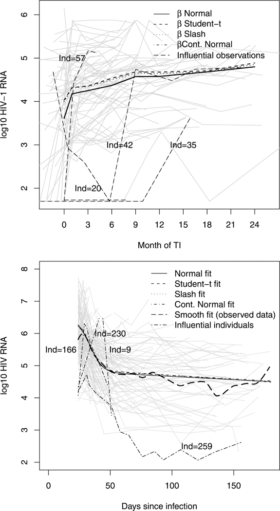
Individual profiles and overall mean (in log₁₀ scale) using the four NI distributions for HIV viral load at different follow-up times for UTI data (upper panel) and AIEDRP data (lower panel). In both the panels, the trajectories for the influential individuals are numbered.

For choice of priors, we have, β_j ~ N₁(0, 10³), j = 1,...,8, σ² ~ IGamma(0.1, 0.1), $\alpha ={\sigma }_b^2~IGamma(0.1,0.1)$; $\nu ~TExp\{0.1;(2,\infty )\}$ for the Student’s-t model, ν ~ Gamma(0.1, 0.01), for the slash model and ν ~ Beta(1, 1) and ρ ~ Beta(2, 2), for the CN model. We generated four parallel independent MCMC runs of size 50,000 with widely dispersed initial values for each parameter for all the four subclasses, where the first 10,000 iterations were discarded as burn-in samples. To eliminate potential problems due to autocorrelation, we considered a spacing of size 20. The convergence of the MCMC chains were monitored using trace plots, autocorrelation plots, and Gelman-Rubin $\widehat{R}$ diagnostics. Sensitivity analysis on the routine use of the inverse-gamma prior on the variance components reveal that the results are fairly robust under different prior choices.

Table 1 compares among the four subclasses of NI models using the model selection criteria discussed in Section 4. Notice that all three members of the NI-LMEC class (with heavy tails) perform significantly better than the N-LMEC, with the CN-LMEC outperforming all the rest. For the T-LMEC and SL-LMEC models, as ν (the t degrees of freedom) → ∞, it approaches the N-LMEC model as a limiting case. For both these models, the estimated value of ν is small, indicating the lack of adequacy of the normal assumption for the UTI data. Posterior densities of ν, along with 95% CI are presented in Web Figure 2. In Table 1, we also report the posterior mean and standard deviations for the model parameters from the four fitted NI models. Note that the posterior estimates of β₁, β₂, and β₃ (the slope parameters corresponding to time points 0, 1, and 3 months) for the NI-LMEC models with heavy tails are quite close to each other and those for the time points further away, i.e., β₄,...,β₈, are also reasonably close to each other. The posterior standard error estimates of (β are small (and consequently have tighter 95% CI) than those in the normal model, indicating that the three heavy-tailed models seem to produce more precise estimates.

Table 1.

UTI data: Comparison between censored normal and NI-LMEC with heavy tails using various model selection criteria and posterior parameter estimates

Criterion	N-LMEC		T-LMEC		SL-LMEC		CN-LMEC
LPML	−423.99		−375.32		−393.37		−365.15
DIC	829.80		726.34		760.58		707.33
EAIC	844.43		749.76		746.39		730.01
EBIC	883.34		792.56		789.20		776.71
Parameter estimates	Mean	SD	Mean	SD	Mean	SD	Mean	SD
${\beta }_1$	3.651	0.126	4.031	0.109	3.999	0.109	3.996	0.102
${\beta }_2$	4.177	0.129	4.314	0.107	4.302	0.109	4.296	0.103
${\beta }_3$	4.247	0.131	4.349	0.108	4.336	0.109	4.326	0.105
${\beta }_4$	4.362	0.132	4.527	0.109	4.492	0.110	4.486	0.105
${\beta }_5$	4.568	0.141	4.672	0.116	4.642	0.116	4.631	0.112
${\beta }_6$	4.584	0.148	4.672	0.120	4.642	0.122	4.627	0.115
${\beta }_7$	4.692	0.165	4.702	0.131	4.677	0.132	4.667	0.127
${\beta }_8$	4.807	0.199	4.884	0.158	4.846	0.157	4.807	0.149
${\sigma }^2$	0.335	0.030	0.122	0.021	0.071	0.011	0.116	0.013
${\sigma }_b^2$	0.782	0.154	0.446	0.109	0.263	0.058	0.446	0.084
$\nu$	-	-	2.621	0.472	1.094	0.086	0.229	0.053
$\rho$	-	-	-	-	-	-	0.095	0.021

With missing-at-random assumption as in Vaida and Liu (2009), our dropout (censored) model does not bias the inference regarding the mean of β_j. The mean viral load E(y_ij) = β_j increases gradually throughout 24 months for all the models. In fact for the CN-LMEC (our best model), it increases from 3.99 with 95% CI (3.89–4.09) at the time of UTI to 4.81 with 95% CI (4.65–4.95) at 24 months. The estimates of the between-subject (${\sigma }_b^2$) and within-subject (σ²) scale parameters (in log₁₀ scale) are 0.446 and 0.116, respectively, which are smaller as compared to the N-LMEC model. To determine possible influential observations, we computed the K-L divergence measures for all the four competing models. From Figure 3 (upper panels) for the N-LMEC, cases 20, 35, 42, and 57 have larger K(P, P_(−i)) as compared to Student’s-t. Web Figure 4 (upper panel) presents K-L plots for the slash and CN models. As expected, the effect of these cases on the posterior estimates of the mean of β were attenuated using the NI class, and hence is a robust alternative for censored viral loads with possible influential observations. This is also observed in Figure 2 (upper panel), where the presence of these outliers might have underestimated the predicted mean curve for the N-LMEC model as compared to the other three NI-LMEC models with heavy tails. The fitted individual viral load trajectories for some randomly chosen subjects using these three models are presented in Web Figure 5.

Figure 3.

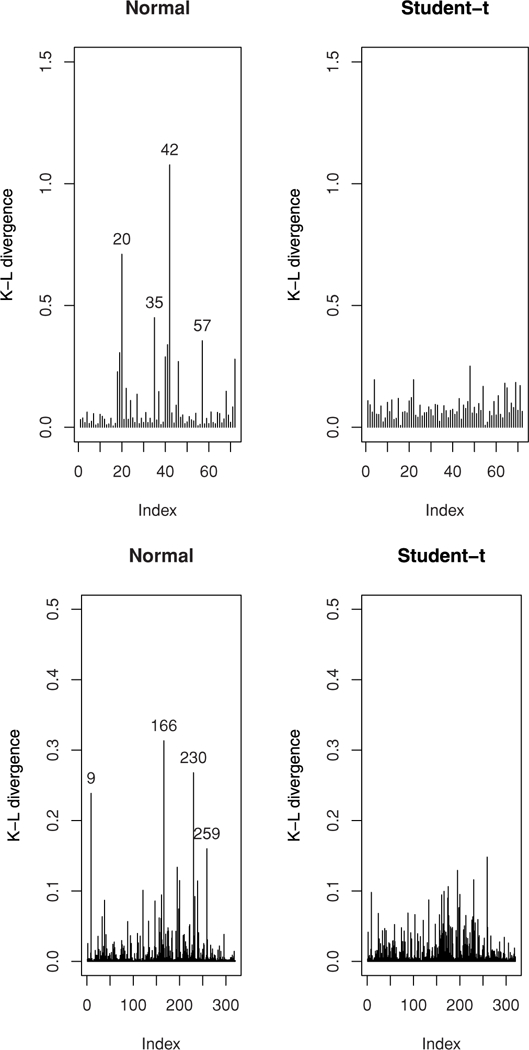
Index plots of K(P, P_(−i)). The upper two plots are for the UTI data whereas the lower two plots are for the AIEDRP data. Influential observations are numbered.

To investigate whether the random effects design matrix should be restricted to only “random intercepts” for the UTI data (as pointed out by a reviewer), we considered two alternative models each with the “time” covariate as in Ho and Lin (2010), given by (i) model 1: y_ij = β₁ + β₂t_ij + b_i + e_ij (random intercept), and (ii) model 2: y_ij = β₁ + β₂t_ij + b_i1 + b_i2 t_ij + e_ij (random intercept and slope). For the best-fitting model (i.e., CN-LMEC), the DIC (LPML) values are 730.77 (−373.93) for model 1 and 807.83 (−412.03) for model 2, respectively, indicating clearly that a simple profile LME model would be adequate.

5.2. AIEDRP Data

The second AIDS case study is from the AIEDRP program, a large multicenter observational study of subjects with acute and early HIV infection. We consider 320 untreated individuals with acute HIV infection; for more details see Vaida and Liu (2009). Of the 830 recorded observations, 185 (22%) were above the limit of assay quantification, hence right censored. So, we consider a right-censored version of (4) and accommodate it within our NLME. Following Vaida and Liu (2009), we choose a five-parameter NLME model (inverted S-shaped curve) as follows:

$$y_{ij}={\alpha }_{1i}+\frac{{\alpha }_2}{\left[1+\exp \left\{\left(t_{ij}-{\alpha }_3\right)/{\alpha }_4\right\}\right]}+{\alpha }_{5i}\left(t_{ij}-50\right)+{ϵ}_{ij},$$

where y_ij is the log₁₀ HIV RNA for subject i at time t_ij. Choice of an appropriate nonlinear model is hard to assess for any HIV data, but the above model was considered in Vaida and Liu (2009) primarily because the residual plots did not exhibit any serial autocorrelation, and the model fit seems adequate. The parameter α_1i and α₂ denotes subject-specific random set points, and the decrease from the maximum HIV RNA, respectively. In the absence of treatment (following acute infection), the HIV RNA varies around a set point, which may differ among individuals; hence the set point is chosen to be subject specific. The location parameter α₃ indicates the time point at which half of the change in HIV RNA is attained, α₄ is a scale parameter modeling the rate of decline and α_5i allows for increasing HIV RNA trajectory after day 50. The smooth (mean) curve for the observed data in Figure 2 (lower panel) agrees with the postulated shape of the HIV RNA trajectory for this study. To force the parameters to be positive, we reparameterize as follows ${\beta }_{1i}=\log \left({\alpha }_{1\text{i}}\right)={\beta }_1+b_{1i}$; ${\beta }_k=\log \left({\alpha }_{\text{k}}\right)$, $k=2,3,4$; and ${\alpha }_{5i}={\beta }_5+b_{2i}$. Within a Bayesian framework, we use the normal (N-NLMEC), Student’s-t (T-NLMEC), SL-NLMEC, and CN-NLMEC models from the NI class, where (b_1i, b_2i) are assumed to be independent and identically distributed (i.i.d.), multivariate NI distributions with unrestricted scale matrix D. The MCMC scheme was similar to the previous application on UTI data, as well as the procedures described in Section 3, further we consider D ~ IWish₂(T⁻¹, 2) with T = Diag (0.01, 0, 0.01).

Table 2 presents comparison among the four subclasses of NI models using various model selection criteria discussed earlier as well as posterior mean and standard deviation of model parameters for the four models. Once again, the NI-NLMEC (with heavy tails) provided much improved model fits over the N-NLMEC, with the Student’s-t outperforming the rest. From Table 2, we observe that the estimates of the slope parameters β₂ and β₄ for the NI models with heavy tails are somewhat different than the normal case. However, the standard errors of the NI-NLMEC are smaller, indicating that the three models with longer tails than normal seem to produce more precise estimates. As earlier, posterior densities of ν and 95% CI are presented in Web Figure 3. Note that for the T-NLMEC and SL-NLMEC, the densities are concentrated around small values of ν, indicating the lack of adequacy of the normality assumption for the model. Similar is the case for the CN-NLMEC model. Henceforth, we consider results based on the Student’s-t distribution (our best model) using the above five-parameter NLMEC model. Residuals plots in our analysis (omitted for brevity) revealed no serial correlations. At 6 months since infection, the estimated average viral load (in logio units) is 4.513, whereas the normal model estimates this at 4.55. The individual 6-month viral load estimates vary between 0.57 and 9.39, with the 95% CI (2.69, 6.55). The average slope after day 50 was negative (β₅ = −0.002) with 95% CI (−0.007, 0.002). This is in contrast to the normal model (Vaida and Liu, 2009), where the 95% confidence interval does not include 0. The individual slopes β₅ + b_i2 included positive values, with 95% CI (−0.014, 0.016). The estimates of the between-subject variance-covariance components D₁₁, D₁₂, and D₂₂ and within-subject scale parameter (σ²) for the NI models (with heavy tails) are slightly smaller as compared to the N-LMEC model. Using the K-L divergence measures, the cases 9, 166, 230, and 259 were identified to be influential (see lower panels of Figure 3 and Web Figure 4) under the N-NLMEC. However, using the NI-NLMEC models, there seem to be no influential observations. We arrive at the same conclusion from Figure 2 (lower panel) that the N-NLMEC might be affected in the presence of outliers. The fitted viral load curve appears to be underestimated as compared to the other three heavy-tailed NI-NLMEC models. Interestingly, estimates of viral load trajectories (Web Figure 5) for some randomly sampled subjects using the NI class are quite distinguishable.

Table 2.

AIEDRP data: Comparison between censored normal and NI-NLMEC with heavy tails using various model selection criteria and posterior parameter estimates

Criterion	N-LMEC		T-LMEC		SL-LMEC		CN-LMEC
LPML	−774.28		−764.77		−772.87		−770.95
DIC	1361.39		1340.48		1352.14		1351.45
EAIC	1546.10		1531.73		1542.01		1538.81
EBIC	1580.02		1569.41		1577.69		1578.26
Parameter	Mean	SD	Mean	SD	Mean	SD	Mean	SD
${\beta }_1$	1.561	0.019	1.575	0.017	1.569	0.019	1.569	0.020
${\beta }_2$	0.478	0.167	0.399	0.143	0.433	0.158	0.439	0.159
${\beta }_3$	3.525	0.052	3.524	0.043	3.522	0.044	3.522	0.040
${\beta }_4$	1.628	0.280	1.414	0.281	1.494	0.301	1.498	0.298
${\beta }_5$	−0.002	0.003	−0.002	0.002	−0.002	0.002	−0.002	0.003
${\sigma }^2$	0.232	0.018	0.186	0.019	0.166	0.028	0.185	0.024
$D_{11}$	0.019	0.003	0.017	0.002	0.014	0.003	0.017	0.003
$D_{12}$	0.0005	0.0003	0.0004	0.0002	0.0004	0.0002	0.0005	0.0002
$D_{22}$	0.0004	0.0001	0.0003	0.0001	0.0003	0.0001	0.0003	0.0001
$\nu$	-	-	9.975	2.8681	5.047	3.955	0.174	0.122
$\rho$							0.405	0.127

6. Simulation Studies

In this section, we conduct a simulation study to investigate the consequences on parameter inference when the normality assumption is inappropriate, as well as to investigate whether the model comparison measures, namely, LPML, DIC, EAIC, and EBIC determine the best-fitting model to the simulated data. We consider the following linear mixed model:

$$\begin{gathered} y_{ij}={\beta }_0+{\beta }_1{t}_{ij}+b_{0i}+b_{1i}{t}_{ij}+{ϵ}_{ij},i=1,\dots ,n(=50), \\ j=1,\dots ,n_i(=6), \end{gathered}$$ (7)

where each subject has been measured at 2, 4, 6, 8, 10, and 24 hours, with a total of six observations per subject (balanced design). We set $\left(b_{0i},b_{1i}\right)\mathbf{\text{i.i.d.}}{T}_2(\mathbf{0},\mathbf{D},\nu )$, ${ϵ}_{ij}~T\left(0,{\sigma }^2,\nu \right)$, ${\mathit{\beta }}^{\top }=\left({\beta }_0,{\beta }_1\right)=(-2.83,-0.18)$, $\mathbf{D}=\left(\begin{array}{cc}0.49& 0.01\\ 0.01& 0.02\end{array}\right),{\sigma }^2=0.15$, and ν = 4.

To study the effect of the level of left censoring in the estimation, we choose three different simulation settings with censoring proportions, say 10%, 20%, and 40%, and simulated 100 datasets for each setting. Next, we fit the LMEC model assuming normal and Student’s-t distributions using R2WinBUGS package available in R. For each of the simulations, we fit the model given in (7) assuming normal and Student’s-t distributions. The following independent priors are considered to perform the MCMC sampling: ${\beta }_k~N_1\left(0,{10}^3\right)$, $k=0,1$; ${\sigma }^2~IGamma(0.1,0.1)$; $\mathbf{D}~IWis{h}_2\left({\mathbf{H}}^{-1},2\right)$ with H = Diag (0.01, 0, 0.01); and ν ~ TExp {0.1;(2, ∞)} for the Student’s-t model. The MCMC scheme follows exactly as in Section 5.1 with respect to number of chains, iteration size, burn-in size, and spacings. For each sample, the posterior parameter mean as well as LPML, DIC, EAIC, and EBIC were recorded. Table 3 presents the summary statistics for β (the fixed-effects parameters) assuming normal and Student’s-t distributions for the three censoring patterns. In these tables, MC mean and MC SD denote, respectively, the arithmetic average of the 100 posterior mean estimates ${\sum }_{j=1}^{100}{\widehat{\theta }}_{kj}/100$ and posterior standard deviations estimates ${\sum }_{j=1}^{100}sd\left({\widehat{\theta }}_{kj}\right)/100$. t-complete indicates the Bayesian estimates for complete data using a Student’s-t model.

Table 3.

Simulation results based on 100 Monte Carlo Student’s-t samples. MC mean and MC SD (in parentheses) are the arithmetic averages of respective posterior mean and standard deviations obtained after fitting NLMEC with Student’s-t and normal densities under different settings of censoring proportions. MC LPML, MC DIC, MC EAIC, and MC EBIC are the arithmetic average of the respective model comparison measures. t-complete indicates Bayesian estimates for complete data using a Student’s-t model.

Censoring	Fit		Simulated Student’s-t data
			β1	β2	σ2	ν	MC LPML	MC DIC	MC EAIC	MC EBIC
10%	Normal	MC Mean	−2.790	−0.187	0.269	-	−367.90	726.30	734.08	565.967
		MC SD	(0.146)	(0.034)	(0.029)
	Student’s-t	MC Mean	−2.794	−0.181	0.174	5.926	−347.415	688.60	698.471	537.347
		MC SD	(0.121)	(0.028)	(0.027)	(1.707)
	t-complete	MC Mean	−2.826	−0.182	0.175	5.781	-	-	-	-
		MC SD	(0.117)	(0.0267)	(0.0261)	(1.653)
20%	Normal	MC Mean	−2.777	−0.194	0.287	-	−339.752	669.058	677.352	699.575
		MC SD	(0.149)	(0.036)	(0.0326)
	Student’s-t	MC Mean	2.799	−0.191	0.173	6.400	−316.984	627.385	638.071	663.998
		MC SD	(0.121)	(0.029)	(0.028)	(2.829)
	t-complete	MC Mean	−2.827	−0.183	0.173	5.824	-	-	-	-
		MC SD	(0.116)	(0.027)	(0.026)	(2.169)
40%	Normal	MC Mean	−2.689	−0.219	0.874	-	−285.287	558.543	569.034	591.258
		MC SD	(0.157)	(0.044)	(0.040)
	Student’s-t	MC Mean	−2.733	−0.209	0.176	7.291	−267.934	527.124	540.277	566.204
		MC SD	(0.131)	(0.033)	(0.033)	(3.849)
	t-complete	MC Mean	−2.827	−0.182	0.174	5.824	-	-	-	-
		MC SD	(0.116)	(0.027)	(0.0258)	(2.173)

From Table 3, we observe that the Student’s-t distribution detects heavy-tailed behavior in the random terms at all levels of censoring, because the estimate of ν is small (at most 7.3). The increase in the proportion of censored data comes with significant bias (the deviations of the parameter estimates from the true values); however, the Student’s-t model shows much less bias and smaller standard deviation estimates as compared to the normal model. Thus, models with “longer-than-normal” tails produce more accurate Bayesian estimates in the context of censored data; the degree and directions of the bias in fixed effects will depend not only on the relative proportions of left (or right) censoring but also on the model assumptions. We also present the arithmetic average (MC LPML, MC DIC, MC EAIC, and MC EBIC) of the various model comparison measures mentioned earlier. All the measures favored the Student’s-t model, demonstrating the ability of these Bayesian measures to detect an obvious departure from normality. This affirmation can be also observed in Web Figure 6, where we plot the values of LPML, DIC, EAIC, and EBIC for the normal and Student’s-t models with 40% censored responses.

7. Conclusions

This article provides a new insight into statistical practices of models and diagnostic methods typically used for analyzing censored HIV viral load outcomes, and presents a useful and practical alternative in presence of thick tails/outliers. For NLMEC, the analysis is computationally feasible through approximating the likelihood function of a NI-NLMEC for a multivariate NI distribution with specified parameters. We apply our methodology to two recent AIDS studies (freely downloadable from R) as well as simulated data to illustrate how the procedures can be used to evaluate model assumptions, identify outliers, and obtain robust parameter estimates. Depending on assay quantifications, we considered both left censoring and right censoring in our setup. We assume the dropout/censoring mechanism to be “missing at random,” (see p. 283 of Diggle et al., 2002); hence in the log-likelihood expression, the observed data component can be separated from the dropout/censoring component. Thus, condition on our model being correct, the dropout does not bias the inference regarding mean viral loads. The models can be fitted using standard available software packages, such as R and WinBUGS (code available upon request) and hence can be easily accessible to practitioners in the field.

Our methods can certainly be extended to interval-censored longitudinal data following Sinha, Chen, and Ghosh (1999). The current framework assumes serially uncorrelated random errors, assuming the sources of randomness (beyond covariates) being primarily attributed to the random effects. Although this assumption appears restrictive (as pointed out by a referee), exploring an appropriate serial correlation structure for random errors warrants further investigation requiring nontrivial modification of the current theoretical framework, which is beyond the scope of this current article. It can also be complicated due to unevenly spaced data, as in our case. The models developed here do not consider skewness in the responses because typically in HIV-AIDS studies, the responses (censored viral load) is log transformed to achieve a “close to normality” shape. However, features of nonnormality might be attributed to both skewness and thick tails, and methods to combine those within a unified framework for censored mixed models are currently under investigation. Incorporating measurement error models (L. Wu, 2010) within our robust framework for related HIV viral load covariates (namely, CD4 cell counts) is also part of our future research.

References

- Cancho V, Dey D, Lachos V, and Andrade M (2011). Bayesian nonlinear regression models with scale mixtures of skew normal distributions: Estimation and case influence diagnostics. Computational Statistics and Data Analysis 55, 588–602. [Google Scholar]
- Carlin B and Louis T (2008). Bayesian Methods for Data Analysis (Texts in Statistical Science). New York: Chapman and Hall/CRC. [Google Scholar]
- Dey DK, Chen MH, and Chang H (1997). Bayesian approach for the nonlinear random effects models. Biometrics 53, 1239–1252. [Google Scholar]
- Diggle PJ, Heagerty P, Liang K-Y, and Zeger SL (2002). Analysis of Longitudinal Data, 2nd edition New York: Oxford University Press. [Google Scholar]
- Dunson D (2001). Commentary: Practical advantages of Bayesian analysis of epidemiologic data. American Journal of Epidemiology 153, 1222–1226. [DOI] [PubMed] [Google Scholar]
- Ho HJ and Lin TI (2010). Robust linear mixed models using the skew-t distribution with application to schizophrenia data. Biometrical Journal 52(4), 449–469. [DOI] [PubMed] [Google Scholar]
- Hobert J and Casella G (1996). The effect of improper priors on Gibbs sampling in hierarchical linear mixed models. Journal of the American Statistical Association 91, 1461–1473. [Google Scholar]
- Hughes J (1999). Mixed effects models with censored data with application to HIV RNA levels. Biometrics 55, 625–629. [DOI] [PubMed] [Google Scholar]
- Jacqmin-Gadda H, Thiebaut R, Chene G, and Commenges D (2000). Analysis of left-censored longitudinal data with application to viral load in HIV infection. Biostatistics 1, 355–368. [DOI] [PubMed] [Google Scholar]
- Lange KL and Sinsheimer JS (1993). Normal/independent distributions and their applications in robust regression. Journal of Computational and Graphical Statistics 2, 175–198. [Google Scholar]
- Lin T and Lee J (2006). A robust approach to t linear mixed models applied to multiple sclerosis data. Statistics in Medicine 25, 1397–1412. [DOI] [PubMed] [Google Scholar]
- Lin T and Lee J (2007). Bayesian analysis of hierarchical linear mixed modeling using the multivariate t distribution. Journal of Statistical Planning and Inference 137, 484–495. [Google Scholar]
- Lindstrom M and Bates D (1990). Nonlinear mixed-effects models for repeated-measures data. Biometrics 46, 673–687. [PubMed] [Google Scholar]
- Liu C (1996). Bayesian robust multivariate linear regression with incomplete data. Journal of the American Statistical Association 91, 1219–1227. [Google Scholar]
- Liu D, Lu T, Niu X, and Wu H (2010). Mixed-effects state-space models for analysis of longitudinal dynamic systems. Biometrics, doi: 10.1111/j.1541-0420.2010.01485.x. [DOI] [PMC free article] [PubMed] [Google Scholar]
- Peng F and Dey DK (1995). Bayesian analysis of outlier problems using divergence measures. The Canadian Journal of Statistics 23, 199–213. [Google Scholar]
- Pinheiro JC, Liu CH, and Wu YN (2001). Efficient algorithms for robust estimation in linear mixed-effects models using a multivariate t-distribution. Journal of Computational and Graphical Statistics 10, 249–276. [Google Scholar]
- Rosa G, Padovani C, and Gianola D (2003). Robust linear mixed models with normal/independent distributions and Bayesian MCMC implementation. Biometrical Journal 45, 573–590. [Google Scholar]
- Russo C, Paula G, and Aoki R (2009). Influence diagnostics in nonlinear mixed-effects elliptical models. Computational Statistics and Data Analysis 53, 4143–4156. [Google Scholar]
- Saitoh A, Foca M, Viani R, Heffernan-Vacca S, Vaida F, Lujan-Zilbermann J, Emmanuel P, Deville J, and Spector S (2008). Clinical outcomes after an unstructured treatment interruption in children and adolescents with perinatally acquired HIV infection. Pediatrics 121, e513–e521. [DOI] [PubMed] [Google Scholar]
- Sinha D, Chen M, and Ghosh S (1999). Bayesian analysis and model selection for interval-censored survival data. Biometrics 55, 585–590. [DOI] [PubMed] [Google Scholar]
- Spiegelhalter DJ, Best NG, Carlin BP, and van der Linde A (2002). Bayesian measures of model complexity and fit. Journal of the Royal Statistical Society, Series B 64, 583–639. [Google Scholar]
- Vaida F and Liu L (2009). Fast implementation for normal mixed effects models with censored response. Journal of Computational and Graphical Statistics 18, 797–817. [DOI] [PMC free article] [PubMed] [Google Scholar]
- Vaida F, Fitzgerald A, and DeGruttola V (2007). Efficient hybrid EM for linear and nonlinear mixed effects models with censored response. Computational Statistics and Data Analysis 51, 5718–5730. [DOI] [PMC free article] [PubMed] [Google Scholar]
- Wu H (2005). Statistical methods for HIV dynamic studies in AIDS clinical trials. Statistical Methods in Medical Research 14, 171–192. [DOI] [PubMed] [Google Scholar]
- Wu L (2010). Mixed Effects Models for Complex Data. Boca Raton, Florida: Chapman & Hall/CRC. [Google Scholar]
Associated Data
This section collects any data citations, data availability statements, or supplementary materials included in this article.