Abstract
This article makes available several genome-wide datasets, which can be used for training microRNA (miRNA) classifiers. The hairpin sequences available are from the genomes of: Homo sapiens, Arabidopsis thaliana, Anopheles gambiae, Caenorhabditis elegans and Drosophila melanogaster. Each dataset provides the genome data divided into sequences and a set of computed features for predictions. Each sequence has one label: i) “positive”: meaning that it is a well-known pre-miRNA, according to miRBase v21; or ii) “unlabeled”: indicating that the sequence has not (yet) a known function and could be a possible candidate to novel pre-miRNA. Due to the fact that selecting an informative feature set is very important for a good pre-miRNA classifier, a representative feature set with large discriminative power has been calculated and it is provided, as well, for each genome. This feature set contains typical information about sequence, topology and structure. Dataset was publically shared in https://sourceforge.net/projects/sourcesinc/files/mirdata/.
Keywords: Bioinformatics, miRNA prediction, Genome-wide data, miRNA features
Specifications table
| Subject area | Bioinformatics |
| More specific subject area | Pre-miRNA prediction |
| Type of data | Tabular data and genomic sequences |
| How data was acquired | Own genome-wide hairpins sequence extractor; and feature extractor miRNAfe[3] |
| Data format | Features in comma-separated-value files and genomic sequences in FASTA format. |
| Data source location | Argentina. |
| Data accessibility | Public repository:https://sourceforge.net/projects/sourcesinc/files/mirdata/ |
Value of the data
|
1. Data
In this work we provide genome-wide hairpins datasets of animals and plants, which can be used as benchmark data for training and testing pre-miRNA predictors. Data consists of a set of FASTA files with folded hairpins sequences of 5 complete genomes:1
-
•
Homo sapiens (hsa),
-
•
Arabidopsis thaliana (ath),
-
•
Anopheles gambiae (aga),
-
•
Caenorhabditis elegans (cel), and
-
•
Drosophila melanogaster (dme).
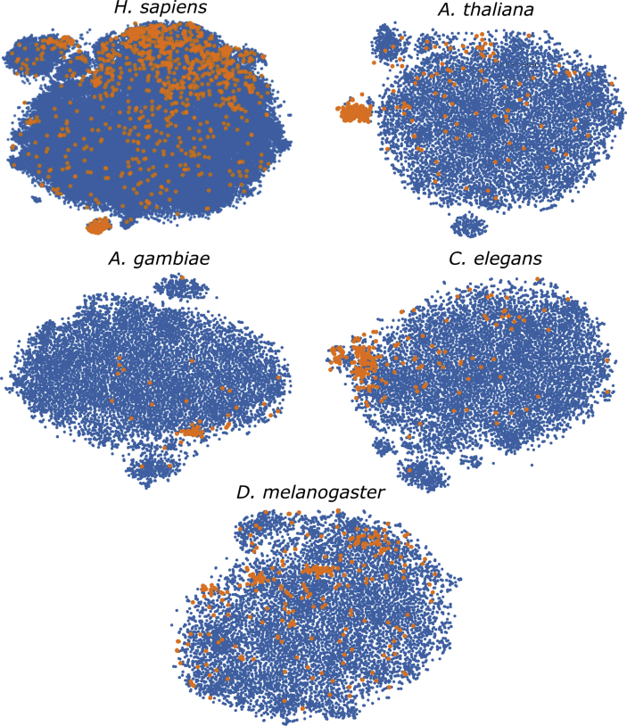
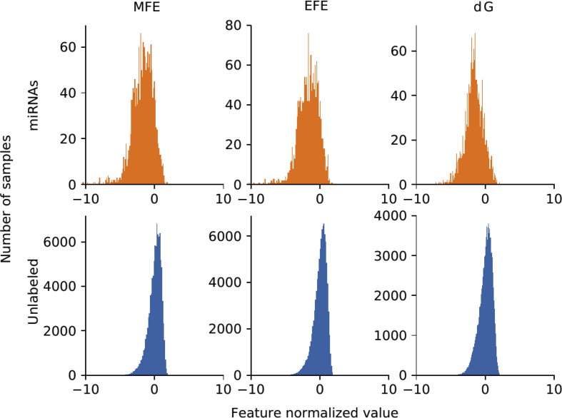
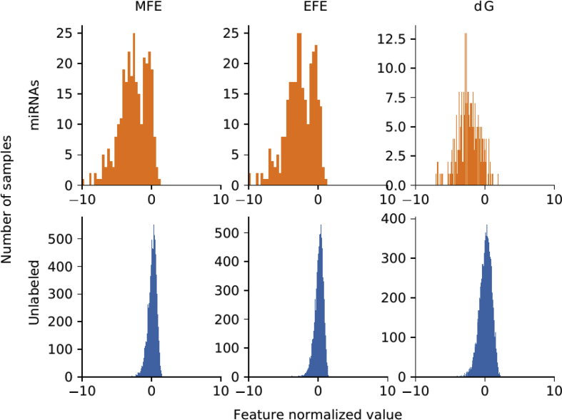
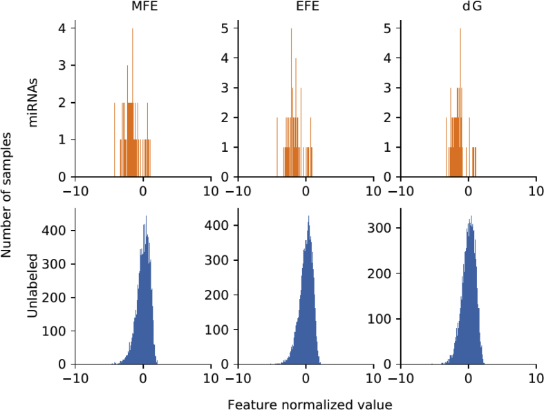
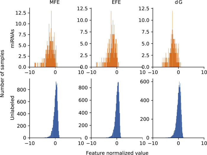
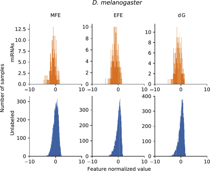
For each genome, there is a set of well known miRNAs sequences, and a larger set of unknown sequences that fold into hairpin structures. Table 1 shows the details of the sequences that have been extracted. For each genome (first column) in the rows, the second column indicates the total number of sequences extracted, which can form hairpins; the third column shows the number of known miRNAs found for each corresponding species. A large number of discriminative features were computed (77 dimensions in total) and stored in.csv files for each genome. The features are listed in Table 2: each row has the feature name, description and dimension (the number of values computed for each feature). A representation of the distribution of the features among positive and unlabeled examples is depicted in Fig. 1. The features values were normalized subtracting the mean and dividing by the corresponding variance and then a t-Distributed Stochastic Neighbor Embedding (t-SNE) [24] was computed. This method generates a 2D projection of the sequences considering the samples neighborhood, based on the similarity of their features. Moreover, Fig. 2, Fig. 3, Fig. 4, Fig. 5, Fig. 6 show the histograms of the normalized features.
Table 1.
Number of stem loops and pre-miRNAs in each genome.
| Species | Extracted hairpins | miRNAs |
|---|---|---|
| H. sapiens | 48,181,565 | 1710 |
| A. thaliana | 1,355,663 | 304 |
| A. gambiae | 4,268,407 | 66 |
| C. elegans | 1,737,349 | 249 |
| D. melanogaster | 2,066,807 | 307 |
Table 2.
Features calculated for each sequence.
| Feature name | Description | Dimension |
|---|---|---|
| nt_proportion | Ratio of each base in the sequence (A, C, G and T) | 4 |
| dinucleotide_proportion | Ratio of dinucleotide elements of each kind, making 16 Features for the possible binary combinations of the 4 nucleotides | 16 |
| gc_content | Proportion of guanine and cytosine on the sequence | 1 |
| gc_ratio | Ratio between guanine and cytosine | 1 |
| sequence_length | The length of the sequence | 1 |
| stem_number | The number of stem-loops | 1 |
| avg_bp_stem | Average of nucleotides per stem | 1 |
| longest_stem_length | Longest region where the pairing is perfect | 1 |
| terminal_loop_length | Number of nucleotides in the stem region | 1 |
| bp_number | Number of base-pairs | 1 |
| dP | Number of base pair divided by the nucleotide number | 1 |
| bp_proportion | Number of each possible base pair normalized by sequence length | 3 |
| bp_proportion_stem | Proportion of base pairs on stems | 3 |
| triplets | Frequencies of secondary structure triplets, this is the 32 possible combinations of the 4 nucleotides in a sequence of 3 | 32 |
| MFE | Minimum free energy | 1 |
| EFE | Normalized Ensemble Free Energy calculated with RNAfold (-p option) | 1 |
| ensemble_frequency | The frequency of the minimum free energy in the ensemble | 1 |
| diversity | Structural diversity calculated with RNAfold (-p option) | 1 |
| mfe_efe_difference | Calculated as |MFE-EFE|/l | 1 |
| dQ | Calculated as 1/L log2pij, where L is length and pij is the probability of pairing of nucleotides i and j | 1 |
| dG | Minimum free energy divided by sequence length | 1 |
| MFEI1 | Ratio between the minimum free energy and the %C+G | 1 |
| MFEI2 | dG/Ns, where Ns is the number of stems. | 1 |
| MFEI4 | MFE/Nb, where Nb is the total number of base pairs in the secondary structure | 1 |
Fig. 1.
t-SNE projection with the well-known pre-miRNAs (in orange) and a random set of unlabeled sequences (in blue) for each genome. Sequences that are closer in the projected feature space have more similar features.
Fig. 2.
Histograms of the top 3 features distributions in H. sapiens: minimum free energy, normalized ensemble free energy (RNAfold) and minimum free energy normalized by length. Well known miRNAs, in orange, have a slightly different distribution but highly overlapped when compared with other sequences (in blue).
Fig. 3.
Histograms of the top 3 features distributions in A. thaliana.
Fig. 4.
Histograms of the top 3 features distributions in A. gambiae.
Fig. 5.
Histograms of the top 3 features distributions in C. elegans.
Fig. 6.
Histograms of the top 3 features distributions in D. melanogaster.
2. Experimental design, materials and methods
The importance of microRNAs (miRNAs) has been largely recognized by the scientific community. MiRNAs on average are about 21 nucleotides long, and take part in the post-transcriptional regulation of gene expression. These short segments of RNA play a role in many fundamental biological processes, such as promoting or inhibiting certain diseases and infections [1]. Precursors of miRNAs (pre-miRNAs, also known as hairpins) are generated during biogenesis and have a very well-known secondary structure: a typical stem-loop structure with few internal loops or asymmetric bulges. Unfortunately, a large amount of hairpin-like structures can be found in a genome [2].
The computational prediction of novel pre-miRNAs involves training a machine learning classifier for identifying candidate sequences for being novel miRNAs. However, to the best of our knowledge, there are no such datasets available. Actually, in most published works, the datasets used for training and testing the prediction methods are manually built, use diverse methodologies according to each study [4], [5], [6], [7], [8], [9], [10], [11], [12], [13], [14], [15], [16], and require a (not negligible) long time. Secondly, it is very hard to fairly compare among different classifiers. Therefore, this makes that published experiments of most pre-miRNA prediction methods cannot be accurately reproduced nor be fully trusted, because the users of those tools cannot obtain the same prediction rates as those published.
In this dataset, we included sequences of model genomes in animals and plants. Although miRNAs may have had a common origin, they had evolved in different ways in the plant and animal kingdoms. The proteins involved in the maturation process of the precursors and the places where it takes place, can be very different. In animals, the transcription of the primary miRNAs (pri-miRNAs) is carried out by RNApol II and RNApol III [17], [18]. After transcription, the pri-miRNAs form stem-loop structures, also called hairpins. These structures are recognized in the nucleus by Drosha and a miRNA precursor (pre-miRNA) is obtained by cleavage. After that, the precursor is exported to the cytoplasm, where it is cut near the terminal loop by the Dicer enzyme, forming a small double-stranded RNA [18]. Some species possess multiple Dicer homologues with different roles. For instance, in D. melanogaster and A. gambiae, Dicer-1 is required for miRNA biogenesis [19]. Following Dicer processing, miRNA is preferentially loaded onto particular types of AGO proteins and the complementary miRNA sequence is discarded. In C. elegans, for example, miRNA duplexes and siRNA duplexes are sorted into ALG-1 and ALG-2 proteins. In humans, by contrast, the four AGO proteins are associated with almost indistinguishable sets of miRNAs because no strict small-RNA-sorting system exists. In plants, the primary miRNAs are transcribed only by RNApol II. In addition, the length of the pri-miRNAs may have a high variation [20]. Unlike the process of the pri-miRNAs in animals, in plants the process of maturation of the miRNAs is carried out completely in the nucleus. This maturation process is not performed by Drosha, because it is not found in plants. Instead, Dicer1-like processes most pri-miRNAs by sequential cleavage in the basal and the apical junctions of the terminal loop [21]. Following this processing, the duplex miRNAs is exported to the cytoplasm. In the cytoplasm, miRNAs are loaded onto cytoplasmic AGO protein [20]. Thus, since the pre-miRNAs biogenesis is different in the animal and plant kingdom, we have included sequences of the species considered as model genomes in these kingdoms.
3. Materials and methods
Each complete raw genome was downloaded from ftp://ftp.ncbi.nlm.nih.gov/genomes/. The input genome-wide data (a multi-fasta file named, for example, genome.fa) is pre-processed with our open-source toolkit HextractoR,2 which automatically extracts and folds all hairpin sequences from raw genome-wide data. It predicts the secondary structure of several overlapped segments, with longer length than the mean length of sequences of interest for the species under processing, ensuring that no one is lost nor inappropriately cut. Then, the prediction of the secondary structures of the sequences obtained was done with the minimum free energy algorithm [22] of RNAfold. After that, miRNAfe [3] was used to extract features for each sequence. Finally, BLAST matching between the extracted sequences and the known miRNAs in miRBase [23] has been done, in order to automatically identify and label those sequences that are, actually, well-known pre-miRNAs.
Each genome has been cut into overlapping windows of a large length (500 nt). This window has been chosen in order to correctly capture a complete hairpin, but also to take into account the neighborhood of any possible hairpin when estimating the secondary structure. This is very important since the results of estimating a secondary structure can be very much affected by the neighborhood of the sequences. Then, the prediction of the secondary structures of the sequences obtained in the previous windowing step has been done. To do this, the minimum free energy algorithm [5] of RNAfold has been used. This algorithm uses dynamic programming for finding the secondary structure that minimizes the energy released. Those hairpins that did not exceed a minimum length of 60 and level pairing of 16 were eliminated.
In order to obtain sequences with lengths similar to those of the well-known pre-miRNA of the particular genome under analysis (found with BLAST matching of the extracted sequences against miRBase), the extracted sequences were trimmed trying to optimize the normalized Minimum Free Energy (NMFE) by the sequence length. The following rules have been applied to achieve this:
-
1.
Each sequence extracted not having a specified minimum length, according to the miRNAs of the genome under analysis, was discarded. This was done in order to ensure that the secondary structure had sufficient length to be a pre-miRNA.
-
2.
The cuts were made in the first unpaired nucleotide of an internal loop or bulge of the secondary structure (starting from the main loop) that passes the minimum length specified. That is, from all unpaired nucleotides, only the ones that are at a certain distance from the main loop are candidates to be a cutting point. It is likely that cutting the sequence at those points will result in a structure with lower NMFE. Moreover, the smaller the length of the sequence (independently of the pairing), the higher the NMFE. Therefore, a loop/bulge closer to the main loop is preferred.
Repeated sequences were eliminated to avoid extra computational cost and because they might also disturb the results of the prediction algorithms, since each repeated sequence increases its relevance for the predictor. Repetitions may appear due to the overlapping in windowing. These repeated sequences appear consecutively and they can be almost identical. To eliminate them, a comparison between each sequence and the last extracted sequence is made. If one of the sequences contains the other one, the shortest one is discarded. Finally, for labeling the sequences obtained, BLAST matching is done against miRBase. The sequences that match, are labeled as positive class (pre-miRNAs).
A characterization of the features of each dataset has been done. A t-SNE projection is shown in Fig. 1. The well-known pre-miRNAs sequences are highlighted in orange, and plotted together with the unlabeled samples in blue. It can be seen that there are some known miRNAs that are close in the projected space. However, there are also many positive samples scattered all over the feature space, showing that accurate prediction is, indeed, a challenging task. This is especially notorious in the H. sapiens and D. melanogaster genomes, which have a very large number of sequences and several well-known miRNAs.
A further insight of the relevance of each feature was done ranking the features according to its importance for classification. Training a random forest [7] with 10 trees, it is possible to see which features are the best ones to separate positive versus unlabeled samples. Taking the average rank across all the genomes, the top-5 most informative features are shown in Table 3. It can be seen that the normalized ensemble free energy (EFE), the minimum free energy (MFE) and its value normalized by length (dG) are the most important features, since those features reflect the stability of the hairpin secondary structure.
Table 3.
Feature relevance.
| Feature | Average rank |
|---|---|
| MFE | 0.40 |
| EFE | 4.20 |
| dG | 6.60 |
| triplets0 | 9.60 |
| MFEI4 | 9.80 |
Fig. 2, Fig. 3, Fig. 4, Fig. 5, Fig. 6 show the histograms of the normalized features, but now analyzed with the top-3 most interesting features of Table 3. They show that features distribution is, indeed, different among positive and unlabeled classes. However, there is a significant overlapping among them, which makes the prediction a challenging task for simple classifiers. This is one of the main motivation for making available to the research community these benchmark datasets: helping and giving support to the proposal of novel and more advanced prediction methods, which could be now fairly compared on the same experimental conditions, such as in [16].
Acknowledgements
This work was supported by Universidad Nacional del Litoral (CAI+D 2011 082) and Agencia Nacional de Promoción Científica y Tecnológica (PICT 2014 2627). We also acknowledged the support of NVIDIA Corporation with the donation of the Titan Xp GPU used for this research.
Footnotes
Conflict of interest
The authors declare that they have no known competing financial interests or personal relationships that could have appeared to influence the work reported in this paper.
References
- 1.Bartel D. MicroRNAs: genomics, biogenesis, mechanism, and function. Cell. 2004;116:281–297. doi: 10.1016/s0092-8674(04)00045-5. [DOI] [PubMed] [Google Scholar]
- 2.Yones C., Stegmayer G., Milone D.H. Genome-wide pre-miRNA discovery from few labeled examples. Bioinformatics. 2018;34:541–549. doi: 10.1093/bioinformatics/btx612. [DOI] [PubMed] [Google Scholar]
- 3.Yones C., Stegmayer G., Kamenetzky L., Milone D.H. miRNAfe: a comprehensive tool for feature extraction in microRNA prediction. Biosystems. 2015;138:1–5. doi: 10.1016/j.biosystems.2015.10.003. [DOI] [PubMed] [Google Scholar]
- 4.Xue C. Classification of real and pseudo microRNA precursors using local structure-sequence features and support vector machine. BMC Bioinf. 2005;6(1):310. doi: 10.1186/1471-2105-6-310. [DOI] [PMC free article] [PubMed] [Google Scholar]
- 5.Hertel J., Stadler P. Hairpins in a haystack: recognizing microRNA precursors in comparative genomics data. Bioinformatics. 2006;22(14):197–202. doi: 10.1093/bioinformatics/btl257. [DOI] [PubMed] [Google Scholar]
- 6.Huang T. MirFinder: an improved approach and software implementation for genome-wide fast microRNA precursor scans. BMC Bioinf. 2007;8(1):341. doi: 10.1186/1471-2105-8-341. [DOI] [PMC free article] [PubMed] [Google Scholar]
- 7.Jiang P. MiPred: classification of real and pseudo microRNA precursors using random forest prediction model with combined features. Nucleic Acids Res. 2007;35(suppl2):339–344. doi: 10.1093/nar/gkm368. [DOI] [PMC free article] [PubMed] [Google Scholar]
- 8.Xu Y., Zhou X., Zhang W. MicroRNA prediction with a novel ranking algorithm based on random walks. Bioinformatics. 2008;24(13):50–58. doi: 10.1093/bioinformatics/btn175. [DOI] [PMC free article] [PubMed] [Google Scholar]
- 9.Gkirtzou K. MatureBayes: a probabilistic algorithm for identifying the mature miRNA within novel precursors. PLoS One. 2010;5(8):11843. doi: 10.1371/journal.pone.0011843. [DOI] [PMC free article] [PubMed] [Google Scholar]
- 10.Gudys A., Szczesniak M., Sikora M., Makalowska I. Huntmi: an efficient and taxon-specific approach in pre-miRNA identification. BMC Bioinf. 2013;14(1):83. doi: 10.1186/1471-2105-14-83. [DOI] [PMC free article] [PubMed] [Google Scholar]
- 11.Ng K., Mishra S. De novo SVM classification of precursor microRNAs from genomic pseudo hairpins using global and intrinsic folding measures. Bioinformatics. 2007;23(11):1321–1330. doi: 10.1093/bioinformatics/btm026. [DOI] [PubMed] [Google Scholar]
- 12.Mendes N., Heyne S., Freitas A., Sagot M.-F., Backofen R. Navigating the unexplored seascape of pre-miRNA candidates in single-genome approaches. Bioinformatics. 2012;28(23):3034–3041. doi: 10.1093/bioinformatics/bts574. [DOI] [PMC free article] [PubMed] [Google Scholar]
- 13.Demirci M., Baumbach J., Allmer J. On the performance of pre-microRNA detection algorithms. Nat. Commun. 2017;8(1):330. doi: 10.1038/s41467-017-00403-z. [DOI] [PMC free article] [PubMed] [Google Scholar]
- 14.Batuwita R., Palade V. microPred: effective classification of pre-mirnas for human mirna gene prediction. Bioinformatics. 2009;25(8):989–995. doi: 10.1093/bioinformatics/btp107. [DOI] [PubMed] [Google Scholar]
- 15.Xue C. Classification of real and pseudo microRNA precursors using local structure-sequence features and support vector machine. BMC Bioinf. 2005;6(1):310. doi: 10.1186/1471-2105-6-310. [DOI] [PMC free article] [PubMed] [Google Scholar]
- 16.Stegmayer G. Predicting novel microRNA: a comprehensive comparison of machine learning approaches. Briefings Bioinf. 2018;bby037 doi: 10.1093/bib/bby037. [DOI] [PubMed] [Google Scholar]
- 17.Ha M., Kim V.N. Regulation of microRNA biogenesis. Nat. Rev. Mol. Cell Biol. 2014;15(8):509. doi: 10.1038/nrm3838. [DOI] [PubMed] [Google Scholar]
- 18.Bartel P. Metazoan MicroRNAs. Cell. 2018;173(1):20–51. doi: 10.1016/j.cell.2018.03.006. [DOI] [PMC free article] [PubMed] [Google Scholar]
- 19.Lee Y.S. Distinct roles for Drosophila Dicer-1 and Dicer-2 in the siRNA/miRNA silencing pathways. Cell. 2004;117:69–81. doi: 10.1016/s0092-8674(04)00261-2. [DOI] [PubMed] [Google Scholar]
- 20.Axtell M.J., Westholm J.O., Lai E.C. Vive la difference: biogenesis and evolution of microRNAs in plants and animals. Genome Biol. 2011;12:221. doi: 10.1186/gb-2011-12-4-221. [DOI] [PMC free article] [PubMed] [Google Scholar]
- 21.Voinnet O. Origin, biogenesis, and activity of plant microRNAs. Cell. 2009;136:669–687. doi: 10.1016/j.cell.2009.01.046. [DOI] [PubMed] [Google Scholar]
- 22.Zuker M., Stiegler P. Optimal computer folding of large RNA sequences using thermodynamics and auxiliary information. Nucleic Acids Res. 1981;9(1):133–148. doi: 10.1093/nar/9.1.133. [DOI] [PMC free article] [PubMed] [Google Scholar]
- 23.Kozomara A., Griffiths-Jones S. miRBase: integrating microRNA annotation and deep-sequencing data. Nucleic Acids Res. 2011;39:152–157. doi: 10.1093/nar/gkq1027. [DOI] [PMC free article] [PubMed] [Google Scholar]
- 24.Maaten L., Hinton G. Visualizing high-dimensional data using t-SNE. J. Mach. Learn. Res. 2008;9:2579–2605. [Google Scholar]


