Locality Sensitive Imputation for Single Cell RNA-Seq Data

Abstract

One of the most notable challenges in single cell RNA-Seq data analysis is the so called drop-out effect, where only a fraction of the transcriptome of each cell is captured. The random nature of dropouts, however, makes it possible to consider imputation methods as means of correcting for dropouts. In this article, we study some existing single cell RNA sequencing (scRNA-Seq) imputation methods and propose a novel iterative imputation approach based on efficiently computing highly similar cells. We then present the results of a comprehensive assessment of existing and proposed methods on real scRNA-Seq data sets with varying per cell sequencing depth.

1. Introduction

Emerging single cell RNA sequencing (scRNA-Seq) technologies enable the analysis of transcriptional profiles at single cell resolution, bringing new insights into tissue heterogeneity, cell differentiation, cell type identification, and many other applications. The scRNA-Seq technologies, however, suffer from several sources of significant technical and biological noise, which need to be addressed differently than in bulk RNA-Seq.

One of the most notable challenges is the so-called drop-out effect. Whether occurring because of inefficient messenger RNA capture or naturally due to low number of RNA transcripts and the stochastic nature of gene expression, the result is capturing only a fraction of the transcriptome of each cell and hence data that have a high degree of sparsity. The dropouts typically do not affect the highly expressed genes but may affect biologically important genes expressed at low levels such as transcription factors. Combining cells as a measure to compensate for the drop-out effects could be defeating the purpose of performing single cell RNA-Seq. In this article, we take advantage of the random nature of dropouts and develop imputation methods for scRNA-Seq. In the next section, we briefly discuss some existing scRNA-Seq imputation methods and propose a novel iterative imputation approach based on efficiently computing highly similar cells. We then present the results of a comprehensive assessment of the existing and proposed methods on real scRNA-Seq data sets with varying sequencing depth.

2. Methods

2.1. Existing single cell RNA-Seq imputation methods

2.1.1. DrImpute

The DrImpute (Kwak et al., 2017) R package implements imputation for scRNA-Seq based on clustering the data. First DrImpute computes the distance between cells using Spearman and Pearson correlations, then it performs cell clustering based on each distance matrix, followed by imputing zero values multiple times based on the resulting clusters, and finally averaging the imputation results to produce a final value for the dropouts.

2.1.2. scImpute

The scImpute (Li and Li, 2017) R package makes the assumption that most genes have a bimodal expression pattern that can be described by a mixture model with two components. The first component is a Gamma distribution used to account for the dropouts, whereas the second component is a Normal distribution to represent the actual gene expression levels. Thus, in Li and Li (2017), the expression level of gene i is considered a random variable with density function , where is the drop-out rate of gene i, and are shape and rate parameters of its Gamma distribution component, and and are the mean and standard deviation of its Normal distribution component. The parameters in the mixture model are estimated using Expectation-Maximization. The authors' intuition behind this mixture model is that if a gene has high expression and low variation in the majority of cells, then a zero count is more likely to be a drop-out value. In contrast, when the opposite occurs, that is, when a gene has constantly low expression or medium expression with high variation, then a zero count reflects real biological variability. According to Li and Li (2017), this model does not assume an empirical relationship between drop-out rates and mean expression levels and thus allows for more flexibility in model estimation.

2.1.3. KNNImpute Troyanskaya et al. (2001)

Weighted K-nearest neighbors [KNNimpute, (Troyanskaya et al., 2001)], a method originally developed for microarray data, selects genes with expression profiles similar to the gene of interest to impute missing values. For instance, consider gene A that has a missing value in cell 1, KNN will find K other genes that have a value present in cell 1, with expression most similar to A in cells , where N is the total number of cells. A weighted average of values in cell 1 for the K genes closest in Euclidean distance is then used as an estimate for the missing value for gene A.

There are also some methods for clustering with implicit imputation, such as BISCUIT Azizi et al. (2017), Prabhakaran et al. (2016), and CIDR Lin et al. (2017). These, however, are out of scope of this article, as we are focusing on stand-alone imputation methods yielding imputed gene expression profiles that can be used for downstream analyses beyond unsupervised clustering, such as dimensionality reduction, counting cells that express known markers, and differential gene expression analysis.

2.2. Proposed method: locality sensitive imputation

We propose a novel algorithm that uses similarity between cells to infer missing values in an iterative approach. The main steps of the algorithm are as follows:

• Step 1. Given a set S of n cells (represented by their scRNA-Seq gene expression profiles), start by selecting pairs of cells with highest similarity level until at least distinct cells ( in our implementation) are selected or the highest pair similarity drops below a given threshold. This process guarantees that each selected cell has highest pairwise similarity level to at least one other selected cell.¹

• Step 2. Cluster the m cells selected in Step 1 using a suitable clustering algorithm (our implementation uses spherical K-means with ). The clusters formed in this step are expected to be “tight,” with each selected cell having high similarity to the other cells in its cluster.

• Step 3. For each of the clusters identified in step 2, replace zero values for each gene j with values imputed based on the expression levels of gene j in all the cells within the cluster.

• Step 4. The selected cells now have imputed values and the clusters they form are collapsed into their respective centroids. The centroids are pooled together with not yet selected cells to form a new set S, and the process is repeated starting again at Step 1.

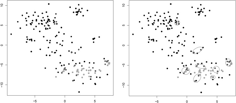
Note that, naturally, in Step 3 expression levels are imputed only for original cells and not for centroids but centroid expression levels are used in the imputation process if they are selected in Step 1. The expression levels used to replace the zero expression values can be inferred through different models. In Section 3 we give results for two simple approaches, namely using the mean, respectively, the median of all expression values for gene j in cells belonging to the cluster (these variants are referred to as LSImputeMean, respectively, LSImputeMed in Section 3). Using the median of both zero and nonzero values first decides implicitly whether a zero is a drop-out event or a true biological effect, and prevents large but isolated expression values from driving imputation of nearby zeros, while collapsing into centroids in each iteration limits the propagation of potential imputation errors. Figure 1 illustrates the first two steps of the algorithm.

FIG. 1.

Illustration of Steps 1 (left) and 2 (right) of LSImpute. Light dots represent already processed cells and collapsed centroids from previous iterations. Darker dots represent cells in pairs with highest similarity level that are selected for clustering.

The worst case number of iterations taken by the algorithm is as the total number of remaining cells and centroids starts at n and decreases by at least one in each iteration. In practice the number of iterations is much smaller. Our current implementation has two options for finding the pairs of cells with highest similarity level in Step 1. The first option is to use Cosine similarity of Hornik et al. (2013). Alternatively, this could be done in time using Jaccard similarity and Locality Sensitive Hashing by Leskovec et al. (2014). Both similarity metrics are available in the Shiny app available at (http://cnv1.engr.uconn.edu:3838/LSImpute/), where the user can also adjust the minimum similarity threshold used in Step 1. It is recommended, however, to use a high similarity threshold, which will restrict the imputation to only highly similar cells as a way of being conservative with imputation to avoid the risk of overimputation. A low similarity threshold can lead to imputing more values and can be used when the data set has a particularly low sequencing depth. All results presented in Section 3 use Cosine similarity and a minimum similarity threshold of 0.85 regardless of sequencing depth to avoid overfitting. Using Jaccard similarity based on the R package LSHR of Selivanov (accessed 2015) resulted in similar imputation levels as the Cosine similarity based implementation.

2.3. Experimental setup

2.3.1. Data sets

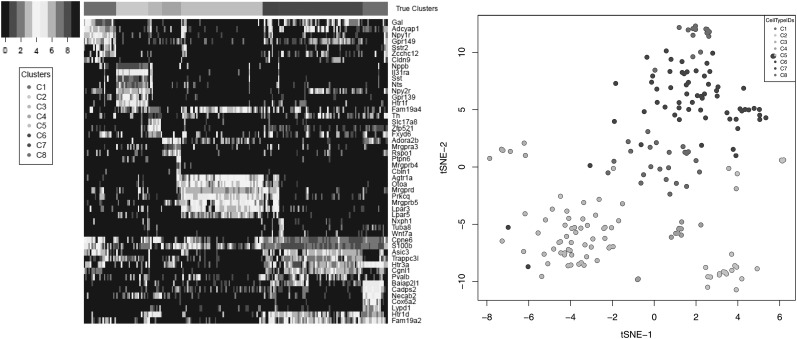
To assess the performance of the compared imputation methods, we used multiple evaluation metrics on data sets consisting of real scRNA-Seq reads down-sampled to simulate varying sequencing depths per cell. Specifically, we used ultradeep scRNA-Seq data generated for 209 somatosensory neurons isolated from the mouse dorsal root ganglion (DRG) and described in Li et al. (2016). An average of 31.5M 2 × 100 read pairs were sequenced for each cell, leading to the detection of an average of genes per cell. To simulate varying levels of drop-out effects, we downsampled the full data set to 50K, 100K, 200K, 300K, 400K, 500K, 1M, 5M, 10M, and 20M read pairs per cell. At each sequencing depth, transcript per million (TPM) gene expression values were estimated for each neuron using the IsoEM2 package by Mandric et al. (2017). As ground truth, we used TPM values determined by running IsoEM2 on the full set of reads. For clustering accuracy evaluation, we used as ground truth the cluster assignment from Li et al. (2016), focusing on the eight cell populations identified using scRNA-Seq data and not its refinement based on neuron sizes (Fig. 2). The C1–C8 clusters we used in this study correspond to the following cell populations identified by their most prominent marker genes as indicated by Li et al. (2016): C1, Gal; C2, Nppb; C3, Th; C4, Mrgpra3 and Mrgprb4; C5, Mrgprd-high; C6, Mrgprd-low and S100b-high; C7, S100b-low; and C8, Ntrk2 and S100b-high.

FIG. 2.

Heatmap of log-transformed TPM values of marker genes identified for DRG neurons in Li et al. (2016; left) and t-SNE plot showing the eight clusters from Li et al. (2016; right). DRG, dorsal root ganglion; t-SNE, t-distributed stochastic neighbor embedding; TPM, transcript per million.

2.3.2. Evaluation metrics

We used the following metrics to evaluate the imputation methods' performance at different sequencing depths:

• Detection fraction accuracy. A common application of single cell analyses is to estimate the percentage of cells expressing a given marker gene, for instance or tumor infiltrating lymphocytes by Duan et al. (2014). A gene is considered to be detected in a cell if the (imputed or ground truth) TPM is positive. For each imputation method, the detection fraction is defined as the number of cells in which the cell is detected divided by the total number of cells. This was compared with the “true” detection ratio, defined based on ground truth TPM values.

• Median percentage error. As defined in Nicolae et al. (2011), the median percentage error (MPE) is the median of the set of relative errors for the gene metric examined, in this case the detection fraction. If a gene has predicted detection fraction y and a ground truth detection fraction of x, the gene's relative error is defined as . For each sequencing depth, we computed MPE relative to all genes as well as subsets of genes corresponding to the four quartiles defined by gene averages of nonzero ground truth TPM values over all cells (ranges of mean nonzero TPM values for the four quartiles were , , and , respectively). Full error curves plotting the percentage of genes with relative error more than varying thresholds were also used for a more detailed comparison of imputation methods.

• Gene detection accuracy. This metric views gene detection as a binary classification problem. For each imputation method, true positives (TPs) are the (gene, cell) pairs for which both imputed and ground truth TPM values are positive, while true negatives (TNs) are (gene, cell) pairs for which both TPM values are zero. The accuracy is computed as the number of true predictions () divided by the product between the number of genes and the number of cells.

• Clustering microaccuracy. For each sequencing depth and imputation method, we clustered imputed TPM values using several clustering algorithms and assessed the effect of imputation on clustering accuracy using the microaccuracy measure by Lee et al. (2011) and Van Asch (2013) defined by , where K is the number of classes, N_i is the size of class i, and C_i is the number of correctly labeled samples in class i relative to the ground truth from Li et al. (2016).

3. Results and Discussion

To assess imputation accuracy on data sets with varying amounts of dropouts, we subsampled the ultradeep DRG scRNA-Seq data to simulate sequencing depths between 50K and 20M read pairs per cell. For each sequencing depth, the metrics described in Section 2.3 were computed for three previous methods (DrImpute, scImpute, and KNNImpute), the two variants of our locality sensitive imputation (LSImpute) method described in Section 2.2 (LSImputeMean and LSImputeMed), and, as a reference, for the “Raw Data” consisting of TPM values without any imputation.

3.1. Detection fraction accuracy

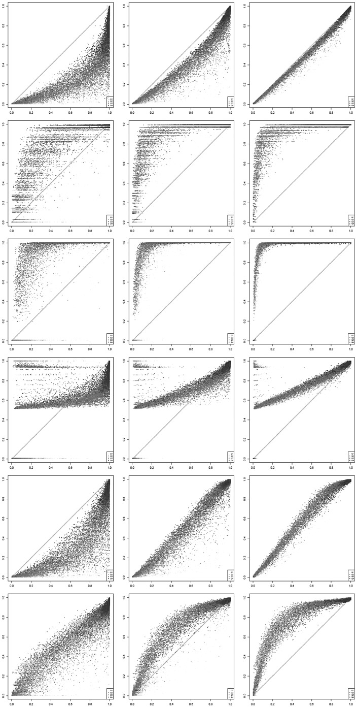
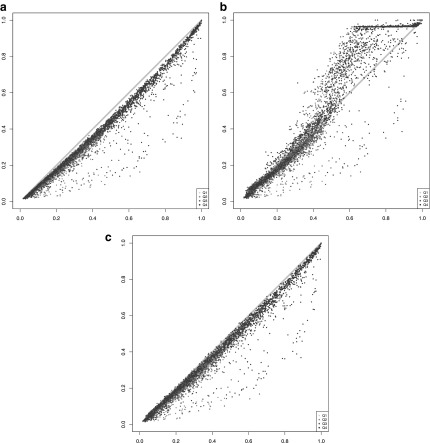
Figure 3 plots the true detection fraction (x-axis) against the detection fraction in the raw data, respectively, after imputation with each of the five compared methods (y-axis) at three selected sequencing depths (100K, 1M, and 10M, respectively, read pairs per cell; high resolution plots for all 10 evaluated sequencing depths are available in the bioRxiv preprint of Moussa and Mandoiu (2018a). Each dot in the scatter plots represents one gene. Dot color shades are based on the four quartiles as defined previously. For an ideal imputation method, all dots would lie on the main diagonal, which represents perfect agreement between predicted and true detection fractions. Dots below the diagonal correspond to genes for which the detection fraction is underestimated, whereas dots above the diagonal correspond to genes for which the detection fraction is overestimated. Dropouts in the raw data yield severe underestimation of the detection fraction for most genes at sequencing depths of 100K and 1M read pairs per cell, but at 10M read pairs per cell, detection fractions computed based on raw data are very close to the true fractions for nearly all genes.

FIG. 3.

True versus imputed detection fractions (left to right: 100K, 1M, and 10M read pairs per cell; top to bottom: raw data, DrImpute, scImpute, KNNImpute, LSImputeMed, and LSImputeMean).

Existing methods overimpute detection fractions for most genes, even at low sequencing depths. At 100K read pairs per cell, LSImputeMed underestimates detection fractions, improving very little over raw values, whereas LSImputeMean gives most accurate detection fractions. At higher sequencing depths, LSImputeMean begins overimputing, whereas LSImputeMed yields most accurate detection fractions at 1M read pairs per cell and only slightly overimputes at 10M read pairs per cell.

3.2. Detection fraction error curves and MPE comparison

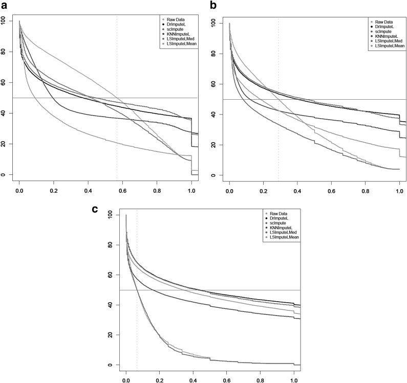
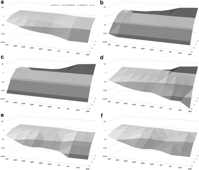
Although dot plots shown in Figure 3 give a useful qualitative comparison of detection fraction accuracy of different methods, for a more quantitative comparison of detection fraction accuracy, Figure 4 shows the so-called error curve of each method. The error curve plots, for every threshold x between 0 and 1, the percentage of genes with a relative error >x. The error curves shown in Figure 4 confirm that LSImputeMean has highest detection fraction accuracy of the compared methods at a sequencing depth of 100K read pairs per cell, whereas LSImputeMed significantly outperforms the other methods at 1M read pairs per cell and matches raw data accuracy at 10M read pairs per cell. The relative performance of the methods can be even more concisely captured by their MPE values, which are the abscissae of the points where the horizontal line with an ordinate of 0.5 crosses the corresponding error curves. The surface plots shown in Figure 5 display MPE values (y axis, on a logarithmic scale) as a function of both sequencing depth (x axis) and mean nonzero expression quartile (z axis). The only imputation methods that do not result in MPE values >100%, depicted in red in the surface plot, are LSImputeMed and LSImputeMean. At all sequencing depths and for all assessed imputation methods, genes in the lowest quartile (Q1) have very high MPE, suggesting that detection fractions based on imputed values should not be used for these genes.

FIG. 4.

Error curves for (a) 100K, (b) 1M, and (c) 10M read pairs per cell. The abscissa of dashed vertical lines corresponds to MPE of raw data. MPE, median percentage error.

FIG. 5.

Surface plots indicating MPE values in log scale (y axis) for each depth (x axis) in each quartile (z axis) for each method: (a) raw data, (b) DrImpute, (c) scImpute, (d) KNNImpute, (e) LSImputeMed, and (f) LSImputeMean

3.3. Gene detection accuracy and relation to MPE

Table 1 gives the gene detection accuracy achieved by the compared imputation methods, with the highest accuracy at each sequencing depth typeset in bold. We assessed gene detection accuracy based on both fractional ground truth and imputed TPM values, as well as after rounding both to the nearest integer, which is equivalent to using a TPM of 0.5 as the detection threshold. For the results without rounding, DrImpute has the highest gene detection accuracy at 50K and 100K read pairs per cell. LSImputeMean has highest gene detection accuracy for 200K read pairs per cell, whereas LSImputeMed outperforms the other methods for 300K–1M read pairs per cell. Raw data (no imputation) give best gene detection accuracy at 5M read pairs per cell and higher depths. For the rounded data sets, DrImpute also has the highest gene detection accuracy at 50K and 100K read pairs per cell, whereas LSImputeMed outperforms the other methods for 200K–500K read pairs per cell. For sequencing depth of 1M read pairs per cell and higher, the raw data give best detection accuracy followed by LSImpute methods.

Table 1.

Gene Detection Accuracy

	Not rounded						Rounded
Data	Raw	Dr.	sc.	KNN.	LSMd	LSMn	Raw	Dr.	sc.	KNN.	LSMd	LSMn
50K	0.676	0.822	0.700	0.799	0.687	0.693	0.752	0.866	0.748	0.700	0.762	0.765
100K	0.740	0.810	0.778	0.713	0.772	0.797	0.816	0.876	0.720	0.712	0.841	0.850
200K	0.800	0.778	0.754	0.726	0.836	0.839	0.872	0.878	0.689	0.722	0.892	0.884
300K	0.829	0.772	0.740	0.732	0.864	0.861	0.899	0.880	0.673	0.726	0.909	0.892
400K	0.847	0.762	0.731	0.736	0.872	0.868	0.915	0.882	0.663	0.730	0.918	0.895
500K	0.859	0.759	0.725	0.738	0.878	0.878	0.927	0.883	0.655	0.732	0.928	0.909
1M	0.891	0.737	0.703	0.747	0.899	0.896	0.952	0.882	0.634	0.738	0.947	0.937
5M	0.918	0.705	0.661	0.762	0.902	0.910	0.980	0.894	0.621	0.772	0.940	0.960
10M	0.920	0.768	0.692	0.648	0.896	0.887	0.987	0.907	0.627	0.800	0.947	0.939
20M	0.921	0.690	0.635	0.774	0.892	0.901	0.994	0.921	0.634	0.825	0.959	0.970

Bold values indicate highest accuracy at each sequencing depth.

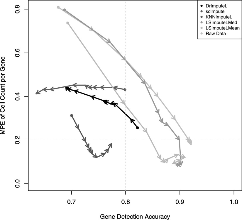
At very low sequencing depth, it is possible for some methods to impute values that are not detected in the ground truth. This could lead to good performance in detection fraction accuracy despite low performance in gene detection accuracy. Furthermore, although one would expect all accuracy measures to improve with increased sequencing depth, this may not necessarily be the case for methods that overimpute. To illustrate the relationship between MPE and gene detection accuracy and the effect of sequencing depth increase, in Figure 6 we plot for each method the gene detection accuracy and MPE achieved without rounding at each sequencing depth from 50K up to 20M read pairs per cell, with consecutive depths connected by arrows pointing in the direction of sequencing depth increase.

FIG. 6.

Gene detection accuracy versus MPE at varying sequencing depths.

Since high accuracy and low MPE are preferable, the points near the lower right corner of the plot and arrows pointing toward it indicate better results. For some methods such as scImpute and DrImpute, although the starting point (50K read pairs per cell) shows considerable improvement over raw data, as sequencing depth increases, one or both of the accuracy measures substantially worsen due to overimputation. Both LSImputeMed and LSImputeMean start with improvement over raw data in both MPE and Gene Detection Accuracy and continue in the right direction for higher depths until, as mentioned before, the raw data without any imputation give slightly better gene detection accuracy at 5M read pairs per cell and higher, which suggests that imputation at such high depths comes with the risk of overimputation for all methods tested.

3.4. Clustering accuracy

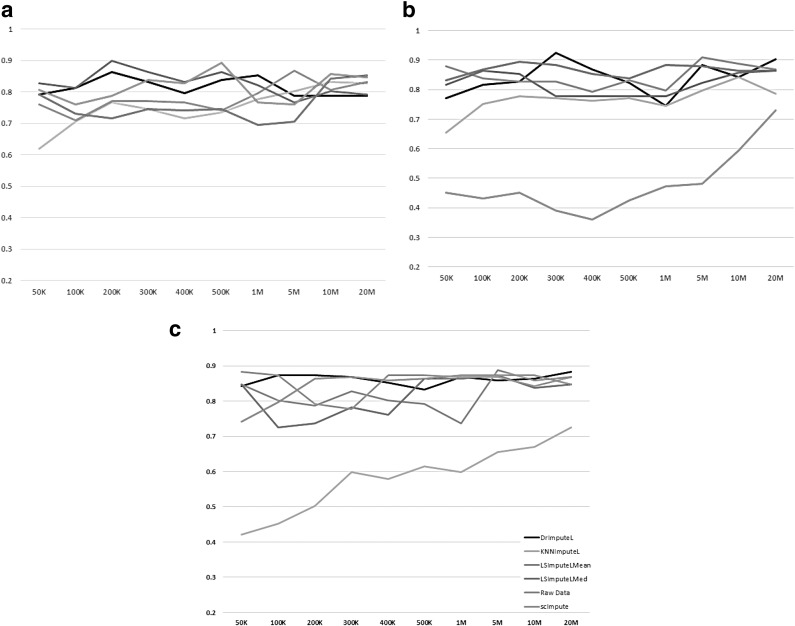
To assess the impact of imputation on clustering results, we tested each of the imputation methods in combination with the following clustering methods: Principal component analysis (PCA)-based hierarchical clustering using Spearman correlation, the TF-IDF_Top_C clustering approach by Moussa and Mandoiu (2018b), and PCA-based spherical k-means clustering. The microaccuracy results shown in Figure 7 suggest that the effect of imputation varies when combined with different clustering approaches. We also tested Seurat Satija et al. (2015) k-means clustering of genes and cells (using with default parameters); however, there was very little change in clustering accuracy for different depths.

FIG. 7.

Microaccuracy on imputed data for (a) PCA-based hierarchical clustering using Spearman correlation, (b) TF-IDF_Top_C Moussa and Mandoiu (2018b), and (c) PCA-based spherical k-means. PCA, principal component analysis.

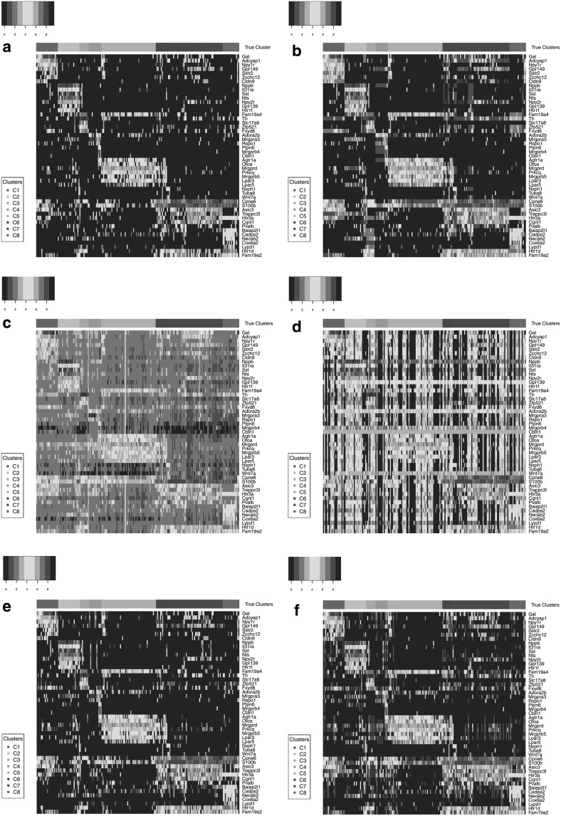
Although the MPE and detection accuracy of some imputation methods suggest that the imputation radically alters gene expression profiles, the similarity between cells of a cluster could still hold when all cell profiles are changed in a consistent manner. This can very well lead to no or little change in clustering accuracy, when in fact cell expression profiles are far from the ground truth as the MPE and gene detection accuracy results suggest. As shown in Figure 8, featuring the expression levels of the marker genes for the DRG 100K data set, although the expression levels of most genes are changed through imputation, the clusters driven by high expression levels of several marker genes can still be the prominent signal for clustering and in most cases this signal remains visually apparent in the heatmaps. Clustering accuracy is hence not recommended as the sole performance evaluation metric when assessing imputation methods.

FIG. 8.

Heatmaps of marker genes from Li et al. (2016) for the 100K DRG data set: (a) raw Data, (b) DrImpute, (c) scImpute, (d) KNNImpute, (e) LSImputeMed, and (f) LSImputeMean.

3.5. Testing LSImpute for 10 × Genomics Technology data

Although the DRG data set is unique in the sense that the ultradeep sequenced version of the scRNA-Seq data can be used as the ground truth for imputation methods testing, we were still able to use a data set from 10 × Genomics Technology platform for testing LSImpute. A library of immune cells, mostly macrophages and natural killer T cells, with an average of 494,275 reads per cell, was downsampled to 52,180 reads per cell (fraction of reads kept is ∼11.8%) by the CellRanger toolkit of 10 × Genomics Cell Ranger™ R Kit Tutorial: Secondary Analysis on 10 × Genomics Single Cell 3 RNA-Seq (n.d.) when combining it with other libraries of the same experiment with lower reads per cell average. As ground truth we used the 500K reads per cell version of the data and we imputed using DrImpute and LSImpute using mean imputation option and 0.75 minimum similarity (we excluded scImpute and KNNImpute due to their consistent overimputation in Section 3).

The gene detection fraction plots for rounded values are shown in Figure 9. The severity of the drop-out effect appears to be lower than for comparable sequencing depths in the DRG set (compare Fig. 9 with the first row of Fig. 3), most likely due to the fact that the “ground truth” for the 10 × data set is itself affected by dropouts. Clearly, overimputation again poses a risk when imputing this data set, as apparent in DRImpute performance, especially for genes detected in higher percentage of the cells as shown in Figure 9b. In contrast, LSImpute imputation approaches the ground truth detection fraction for all genes with negligible overimputation as shown in Figure 9c. The gene detection accuracy is 0.970 for the raw reads, 0.950 for DrImpute, and 0.974 for LSImpute.

FIG. 9.

Detection fraction plots of 10 × leukocytes set of 638 cells. (a) 500K(true) versus 50K(downsampled) reads per cell. (b) True versus DrImpute imputed detection fractions. (c) True versus LSImputeMean detection fractions.

4. Conclusion

Although imputation can be a useful step in scRNA-Seq analysis pipelines, it can become a two-edged sword if expression values are overimputed. In this article, we evaluated the performance of several existing imputation R packages and presented a novel approach for imputation. LSImpute, especially the variant based on median imputation, tends to impute more conservatively than existing methods, resulting in improved performance based on a variety of metrics. Overall, LSImpute is more likely to reduce drop-out effects and reduce sparsity of the data without introducing false expression patterns or overimputation. Cosine and Jaccard similarity based implementations of LSImpute are available as a Shiny app at (http://cnv1.engr.uconn.edu:3838/LSImpute).

Author Disclosure Statement

I.I.M. is a cofounder and holds an interest in SmplBio LLC, a company developing cloud-based scRNA-Seq analysis software. No products, services, or technologies of SmplBio have been evaluated or tested in this study.

References

- Azizi E., Prabhakaran S., Carr A, et al. 2017. Bayesian inference for single-cell clustering and imputing. Genom. Comput. Biol. 3, 46 [Google Scholar]
- Cell Ranger™ R Kit Tutorial: Secondary Analysis on 10 × Genomics Single Cell 3 RNA-Seq PBMC Data (n.d). 10x Genomics, July 18, 2017 [Google Scholar]
- Duan F., Duitama J., Al Seesi S., et al. 2014. Genomic and bioinformatic profiling of mutational neoepitopes reveals new rules to predict anticancer immunogenicity. J. Exp. Med. 211, 2231–2248 [DOI] [PMC free article] [PubMed] [Google Scholar]
- Hornik K., Feinerer I., Kober M., et al. 2013. Spherical k-means clustering. J. Stat. Softw. 50, 1–22 [Google Scholar]
- Kwak I.-Y., Gong W., Koyano-Nakagawa N., et al. 2017. DrImpute: Imputing dropout events in single cell RNA sequencing data. bioRxiv 181479 [DOI] [PMC free article] [PubMed] [Google Scholar]
- Lee C., Măndoiu I.I., and Nelson C.E. 2011. Inferring ethnicity from mitochondrial DNA sequence. BMC proceedings, Vol. 5, BioMed Central, S11. [DOI] [PMC free article] [PubMed] [Google Scholar]
- Leskovec J., Rajaraman A., and Ullman J.D. 2014. Mining of Massive Datasets. Cambridge University Press [Google Scholar]
- Li C.-L., Li K.-C., Wu D., et al. 2016. Somatosensory neuron types identified by high-coverage single-cell RNA-sequencing and functional heterogeneity. Cell Res. 26, 83. [DOI] [PMC free article] [PubMed] [Google Scholar]
- Li W.V., and Li J.J. 2017. scImpute: Accurate and robust imputation for single cell RNA-seq data. bioRxiv 141598. [DOI] [PMC free article] [PubMed] [Google Scholar]
- Lin P., Troup M., and Ho J.W. 2017. CIDR: Ultrafast and accurate clustering through imputation for single-cell RNA-Seq data. Genome Biol. 18, 59. [DOI] [PMC free article] [PubMed] [Google Scholar]
- Mandric I., Temate-Tiagueu Y., Shcheglova T., et al. 2017. Fast bootstrapping-based estimation of confidence intervals of expression levels and differential expression from RNA-Seq data. Bioinformatics. 33, 3302–3304 [DOI] [PubMed] [Google Scholar]
- Moussa M., and Mandoiu I. 2018a. Locality sensitive imputation for single-cell RNA-Seq data. bioRxiv. 291807 [DOI] [PMC free article] [PubMed] [Google Scholar]
- Moussa M., and Mandoiu I. 2018b. Single cell RNA-Seq data clustering using TF-IDF based methods. BMC Genom. 196, pg. 127. [DOI] [PMC free article] [PubMed] [Google Scholar]
- Nicolae M., Mangul S., Mandoiu I.I., et al. 2011. Estimation of alternative splicing isoform frequencies from RNA-Seq data. Algorithms Mol. Biol. 6, 9. [DOI] [PMC free article] [PubMed] [Google Scholar]
- Prabhakaran S., Azizi E., Carr A., et al. 2016. Dirichlet process mixture model for correcting technical variation in single-cell gene expression data. International Conference on Machine Learning, 1070–1079 New York, NY [PMC free article] [PubMed] [Google Scholar]
- Satija R., Farrell J.A., Gennert D., et al. 2015. Spatial reconstruction of single-cell gene expression data. Nat. Biotechnol. 33, 495. [DOI] [PMC free article] [PubMed] [Google Scholar]
- Selivanov D. accessed 2015. dselivanov/lshr. Available at: https://github.com/dselivanov/LSHR
- Troyanskaya O., Cantor M., Sherlock G., et al. 2001. Missing value estimation methods for DNA microarrays. Bioinformatics. 17:520–525 [DOI] [PubMed] [Google Scholar]
- Van Asch V. 2013. Macro-and micro-averaged evaluation measures. Tech. Rep [Google Scholar]