Large-Scale Heterogeneous Representation of Sound Attributes in Rat Primary Auditory Cortex: From Unit Activity to Population Dynamics

Abstract

Recent evidence indicates the existence of pyramidal cells (PCs) and interneurons with nontrivial tuning characteristics for sound attributes in the primary auditory cortex (A1) of mammals. These neurons are functionally distributed into layers and sparsely organized at a small scale. However, their topological locations at a large scale in A1 have not yet been investigated. Furthermore, these neurons are usually classified from fine maps of attribute-dependent spiking activity, and not much attention is paid to population postsynaptic potentials related to their activity. We used extracellular recordings obtained from multiple sites in A1 of adult rats to determine neuronal codifiers for sound attributes defined by coarse representations of the population dose–response curves. We demonstrated that these codifiers, majorly involving PCs, are heterogeneously distributed along A1. Spiking activity in these neurons during stimulation was correlated to β (12–25 Hz) and low γ (25–70 Hz) postsynaptic oscillations in the infragranular layer, whereas in the supragranular layer, better correlations were found with high γ (70–170 Hz) oscillations. The time-frequency analysis of the postsynaptic potentials showed a transient broadband power increase in all layers after the stimulus onset that was followed by a sustained high γ oscillation in the supragranular layer, fluctuations in the laminar content of the low-frequency oscillations, and a global attenuation in the low-frequency powers after the stimulus offset that happened together with a long-lasting strengthening of the β oscillations. We concluded that, for rats, sounds are codified in A1 by segregated networks of specialized PCs whose postsynaptic activity impinges on the emergence of sparse/dense spiking patterns.

Introduction

Perceptual dimensions in human audition (i.e., timbre, pitch, and loudness) are determined by three fundamental attributes of a sound, i.e., the frequency, the amplitude, and the time envelope of harmonic composition. The codification of these attributes has been thought to occur by means of spatially distributed assemblies of neurons exhibiting attribute-dependent response curves. The threshold-based tonotopic gradient for frequency codification in the primary auditory cortex (A1) constitutes the most accepted spatial segregation of a sound attribute in mammals [cats (Woolsey and Walzl, 1942), rats (Sally and Kelly, 1988)]. Monotonic neurons, presumably used for such a construction, show a V-shaped frequency response area (FRA) with the spectral bandwidth Q₁₀ (Q₄₀) for the near (away) response threshold. Quite the opposite, suprathreshold stimulation at a single frequency created patchy activation patterns extended over the entire A1 (Bakin et al., 1996).

Recently, nonmonotonic coding schemes in A1 (i.e., neurons with an O-shaped FRA), known as intensity tuning, have been proposed for both level-invariant representations (Sadagopan and Wang, 2008) and low-level codifications (Watkins and Barbour, 2011). In cats and monkeys, monotonic neurons are spatially segregated from those that are nonmonotonic (Sutter and Schreiner, 1995; Recanzone et al., 2000; Linden and Schreiner, 2003). Still, it needs to be clarified whether the same or different neuronal assemblies take part in codifying sound time envelopes through a spatial segregation strategy. Some studies have reported a pitch-selective area near the low-frequency border of A1 [monkeys (Bendor and Wang, 2005, 2010), ferrets (Bizley et al., 2009, 2010)], whereas others claim peculiar spatial organizations [e.g., Mongolian gerbils, circular gradient (Schulze et al., 2002); cats, linear gradient (Langner et al., 2009)]. Neurons sensitive to the modulation frequency are uniformly distributed in A1 [rats (Kilgard and Merzenich, 1999), monkeys (Bendor and Wang, 2005, 2010)].

Considering both the diversity of FRA patterns and the spatial heterogeneity of neurons codifying sound attributes in A1 for several species, it seems imprecise to use searching strategies based on classical schemes for sound representation (i.e., independent neurons with simple tuning effects clearly distributed in A1). The existence of nonclassical schemes may be in line with findings reported recently: (1) complex FRA maps (Schreiner et al., 2000; Gaese and Ostwald, 2003; Turner et al., 2005); (2) inhibitory sideband effects (O'Connell et al., 2011); (3) high variability along cortical layers (Wallace and Palmer, 2008; Sakata and Harris, 2009; Hackett et al., 2011); and (4) sparseness activation patterns (Hromádka et al., 2008; Sakata and Harris, 2009; Rothschild et al., 2010). Therefore, to study the neuronal substrates for sound attribute codification in A1 of Wistar rats, we chose to apply a simple but complementary approach that is based on a massive exploration of a large cortical sheet at all depths. To that end, the strategy to determine the neuronal codifiers was founded on coarse representations of the population pairwise attribute response curves. For these codifiers, we explored (1) the topological distributions, (2) the current source density (CSD)–spike relationships during ongoing/stimulus-related activity, and (3) the unit activity/oscillatory laminar profiles.

Materials and Methods

All procedures and protocols were performed in agreement with the policies established by the Animal Care Committee at Tohoku University (Sendai, Japan). Animal experiments were performed on 8- to 12-week-old male Wistar rats (287–386 g; n = 5).

Homemade three-dimensional probe.

While studying the topological characteristics of the neuronal response in A1 to auditory stimuli, researchers subsequently insert electrodes in different cortical locations, e.g., tungsten microelectrodes (Doron et al., 2002; Rutkowski et al., 2003) and silicon-based laminar (Sakata and Harris, 2009) and planar (Lakatos et al., 2007; Bizley et al., 2009, 2010) probes. This strategy has two major drawbacks: (1) the tissue condition deteriorates with each insertion and (2) it is hard to evaluate the actual probe location because of successive contractions/expansions of a small cortical area that may occasionally induce tissue swelling and bleeding. To avoid cortical damage or imprecision in the placement of the electrodes caused by a multiple penetration strategy, and thus bias our results, in this study we preferred to obtain simultaneous laminar recordings from several places in A1 using a single insertion strategy. To that end, we created a 3-D probe that consisted of two planar acute silicon-based probes (a4×8-5mm100-400-177; Neuronexus Technologies) tightly attached together with superglue. Each planar probe comprises 32 channels (eight active sites on four parallel shanks, with a vertical spacing of 100 μm; microelectrode area, 177 μm²). With the help of the S6D microscope (Leica), these two probes were assembled by hand in such a way that the shanks of both probes were parallel and their tips approximately aligned. The distance between the planar probes for all experiments was 450 ± 50 μm.

Magnetic resonance imaging and coregistration to a Wistar rat atlas.

Magnetic resonance imaging (MRI) data were acquired using a 7 tesla Bruker PharmaScan system (Bruker Biospin) with a 38-mm-diameter birdcage coil. Each rat was initially anesthetized with 5% isoflurane and then secured on a custom-built holder using adhesive tape and a bite bar. A breathing sensor (SA Instruments) was placed under the ventral face of the rat body. Anesthesia was further maintained with isoflurane (at 1 L/min oxygenation) administered via a face mask. A constant breathing rate was maintained around 50 breaths per minute during the entire MRI acquisition by manually keeping the concentration of isoflurane between 1.5 and 2.5%. Core body temperature was kept at 37.0 ± 1°C by means of a hot water-circulating pad. The high-resolution T2-weighted images were obtained using a respiratory-gated, 2-D TurboRARE sequence with fat suppression (TR, 4628 ms; TE, 30 ms; effective spectral bandwidth, 100 kHz; flip angle, 90°; field of view, 32 × 32 mm²; matrix size, 256 × 256; in-plane resolution, 125 × 125 μm²; number of slices, 54; slice thickness, 0.5 mm; slice gap, 0 mm; number of averages, 10). The total scanning time for T2-weighted imaging was ∼50 min, depending on the respiration rate for each rat. T2-weighted images were normalized to the rat brain atlas template (P. A. Valdés-Hernández, A. Sumiyoshi, H. Nonaka, R. Haga, E. Aubert-Vásquez, T. Ogawa, Y. Iturria-Medina, J. Riera, and R. Kawashima, unpublished observations), which was, by construction, coregistered to a digitalized atlas (Paxinos and Watson, 2007). The normalized T2-weighted images were converted back to the native space allowing us to estimate the actual extension of A1 in the individual rat brain and the relative position of its center in the atlas coordinate space [Fig. 1A, left (axial slice) and middle (coronal slice)]. The actual positions of two crucial landmarks for stereotaxic-guided craniotomy in rats, i.e., the bregma and the lambda, were also determined from the individual T2-weighted images. In the same way, we calculated the approximate point (P_A1) where the A1's center projects perpendicularly to the anteroposterior axis defined by these landmarks, a step that allowed us to determine the lateral distance from the sagittal suture to the center of the surface of A1. Based on the MRI data, we planned the site for the craniotomy as illustrated in Figure 1A (right).

Figure 1.

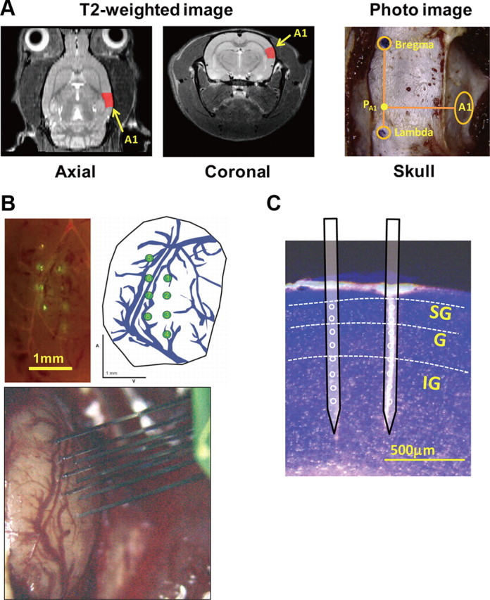
Localization of the A1 based on MRI guidance and colocalization of the shanks. A, Rat brain T2-weighted images of the axial slice (left) and the coronal slice (center). Individual T2-weighted images were coregistered to the atlas coordinate space (presurgery). Based on the coregistration, we developed a strategy for stereotaxic/MRI guidance, i.e., the bregma, the lambda, and P_A1, and the A1 were localized accurately (right) on the exposed skull (during surgery). In the T2-weighted images, the red color shows the right A1 coregistrated to the Paxinos and Watson (2007) atlas. B, Colocalization of the shanks based on the vessel distribution, as revealed by fluorescent staining. A fluorescent image (top left) shows the shank positions (yellow green) and the vessel distribution (bright red) in A1. A sketch with the distribution of principal vessels was obtained from a photograph captured by the digital microscope (top right, green circle: position of the shank). C, Laminar structure of the A1 and the colocalization of the shanks. Based on the Nissl staining, the isocortex in the A1 was divided into three parts, SG, G, and IG layers. The thickness of the layers were in correspondence, with certain inter-rat variability, to a previous study (SG, 29%; G, 10%; IG, 48%; Games and Winer, 1988).

Surgical procedures.

In the electrophysiological experiments, anesthesia was induced with urethane (1.2 g/kg). The animals were placed on a stereotaxic stage, and the temporal muscles on right side were retracted. A craniotomy was performed over A1 based on MRI guidance, and the accuracy of the method was later confirmed by the vessel distribution (Fig. 1B, top right). The dura was removed under the digital microscope KH-1300 (Hirox), and the cortex was covered with HEPES-buffered and Ca²⁺-free aCSF (150 mm NaCl, 2.5 mm KCl, 1 mm MgCl₂ · 6H₂O, 10 mm HEPES, 10 mm glucose; the pH was adjusted to 7.4 with Tris base). Two screws, used as the reference and the ground for the extracellular recordings, were attached to the skull close to the lambda point (Riera et al., 2010).

Electrophysiological recordings.

The insertion length and angle of the 3-D probe were accurately monitored/corroborated through a micromanipulator's control system (SM5; Luigs & Neumann). The 3-D probe was perpendicularly inserted 1050 μm into the cerebral cortex. Therefore, it observes neuronal activity from the region between 250 and 1050 μm in depth. The values of microelectrode impedance in the probe ranged between 0.7 and 0.9 MΩ.

Extracellular potentials were recorded using amplifiers at 25 kHz (PZ2; Tucker-Davis Technologies) connected by an optical fiber to a signal processing unit that comprises eight parallel central processing units (RZ2, Tucker-Davis Technologies) and by a coaxial cable to a preamplifier located inside two acute 32-channel, 18-bit hybrid headstages, respectively. By means of the 3-D probe, we were able to simultaneously record extracellular potentials from eight different sites along the A1 surface for each rat, a total of 64 channels (Fig. 1B, bottom). All recordings were performed using an on-line logic/symbolic programming language supported by the signal processing unit (OpenEx software; Tucker-Davis Technologies).

Auditory stimulation protocol.

Acoustic stimuli were generated digitally by a custom-written code in MATLAB (R2009b; The MathWorks) and delivered with a digital-to-analog converter (National Instruments) and a speaker driver (ED1; Tucker-Davis Technologies) to a calibrated condenser speaker (ES1; Tucker-Davis Technologies). Anesthetized animals placed inside a single-walled soundproof box (VIC International) were stimulated through a customized ear tube inserted into the left ear canal. Speaker calibration was conducted using a condenser microphone (UC-29; Rion) close to the tip of the ear tube. The frequency-dependent gain for the speaker used in all our experiments was almost constant within the frequency band of interest (8–40 kHz) with a mean value 101 ± 6 dB SPL (±4 V speaker input). Acoustic stimuli consisted of amplitude-modulated sounds (200 ms long) presented 10 times with an interstimulus interval of 1.6 s (Langner et al., 2009). The coarse scale (k = 1,2,3) for the attribute values was defined as follows: carrier frequency f_c (kHz) = (2k − 1) × 8; modulation frequency f_m (Hz) = 10^{0.602×(k−1)} × 50; peak of amplitude Amp (dB SPL) = 30 + (k − 1) × 20. For each stimulation block, 27 acoustic stimuli, henceforth called conditions, were randomly prepared from combinations of these attribute values (Table 1). The final stimulation protocol for each rat comprised 10 consecutive blocks. A total of 100 trial-evoked potentials were recorded in each condition. To illustrate the correspondence between the fine and coarse scales when representing the dose–response curves, we used the following attribute values for one rat: f_c (kHz) = k × 8, f_m (Hz) = 10^{0.301×(k−1)} × 50, and Amp (dB SPL) = 30 + (k − 1) × 10; with k = 1, …, 5.

Table 1.

Attributes for the auditory stimuli

		V1	V2	V3
A1	Frequency (fc)	8 kHz	24 kHz	40 kHz
A2	Amplitude (Amp)	30 dB	50 dB	70 dB
A3	Modulation (fm)	50 Hz	200 Hz	800 Hz

A, Type of attribute, V, value of attribute.

Histology.

To colocalize the shanks of the 3-D probe, DiO dye (Invitrogen) was gently applied on the backside surface of the shank before insertion. After the electrophysiological experiments, each rat was perfused transcardially with 10 ml of PBS and 10 ml of PBS with 200 μl of DiI (Invitrogen) for vessel staining and fixed with 10 ml of 4% paraformaldehyde (Li et al., 2008). Finally, the brain was removed and postfixed in the same fixative through the night at 4°C. Fluorescent images (Fig. 1B, top left) containing information about the shank positions (yellow-green) and the vessel distribution (bright red) were captured with an upright fluorescent microscope (SZX16; Olympus). A sketch with the distribution of principal vessels was produced for each rat (Fig. 1B, top right). Coronal sections (100 μm thickness) from the entire A1 were obtained from the postfixed brains with Vibratome 1000-plus (Leica). Fluorescent Nissl staining for each brain section was additionally performed (Goto et al., 2010). Nissl staining images, colocalized with the shank traces, were obtained with the SZX16 microscope (Fig. 1C).

Preprocessing of the electrophysiological data.

The extracellular potentials were processed by a custom-written code in MATLAB (R2009b; The MathWorks). Local field potentials (LFPs) and multiunit activity (MUA) were separated by low-frequency (1–170 Hz) and high-frequency (500–5000 Hz) Butterworth IIR type bandpass filters, respectively. Single-trial auditory-evoked potentials (AEPs) were estimated from the LFPs using the stimulus triggers, which were also recorded by an extra analog channel.

MUA analysis: population codifiers of sound attributes.

Spike sorting was performed off-line. We used a free downloaded toolbox, Wave Clus, for the semiautomatical detection of spikes (Quiroga et al., 2004). An amplitude threshold of 3.5 SD of the mean amplitude was used for spike detection in each channel (Rasch et al., 2011), which is recommended to reduce the number of missed spikes in the particular case of data with high noise levels (i.e., the SD of the noise relative to the amplitude of the spikes, ∼40% for our MUA data). This implied an increase in the number of false positives that were easily recognized by visual inspection. We used both positive and negative thresholds to improve the spike detection accuracy and, as suggested by Quiroga et al. (2004), to account for any spike class with opposite polarity. As a result of the existence of a refractory period, any spike occurring 1.5 ms after a preceding spike was ignored (Whittingstall and Logothetis, 2009). The window used to evaluate the spiking rate in each microelectrode was 10 ms in size, and it moved in 1 ms steps. To identify possible cortical sites for attribute codification, first the MUAs for the eight channels on the same shank (i.e., population spiking rate) were integrated, and the result was normalized with respect to the maximal population spiking activity in the 3-D probe for that particular stimulus condition (Fig. 2A, 8 kHz, 50 Hz, 70 dB). After that, a respective interpolated topographic map was created from this normalized/integrated MUA in all shanks at 15 ms after stimulus onset (Fig. 2B). The maximum of the population spiking activity was always reached at this particular time instant. To define a particular codifier, the normalize/integrated MUA was compared for different conditions (Fig. 2C; the eighth shank contains information about a neuronal population codifying the amplitude of the tone with a carrier frequency of 8 kHz and modulated at 50 Hz).

Figure 2.

An example of the MUA analysis for the identification of a single codifier (Amp). A, Left, One hundred-trial raster plots (black dot) and the evoked population spike rates (normalized, blue lines) for each shank. Spikes were detected in all electrodes (eight sites) on each shank. Each row corresponds to data from a particular shank with spikes from all electrodes overlapping. The stimulus conditions in this example were as follows: f_c, 8 kHz; f_m, 50 Hz; Amp, 70 dB SPL. The red line identifies the time instant of interest for attribute codification in our study, i.e., 15 ms after stimulus onset, which constitutes the peak of the population spiking activity. B, The topological mapping of the normalized/integrated MUA, obtained at that particular time instant, is illustrated. The black rhombus represents the position of the shanks. A color bar is used to represent the level of normalized/integrated MUA. C, Normalized/integrated MUA for different sound amplitudes (blue, 30 dB; green, 50 dB; red, 70 dB; window for counting spikes, 10 ms; moving step, 1 ms). The spikes were classified from data at shank-8 (B, yellow circle). Codifiers of sound attributes were identified from the normalized/integrated MUA 15 ms after the stimulus onset (vertical black line); hence, these codifiers represent transient encoders for all sound attributes. In A and C, the stimulus interval is represented by bold black lines (duration, 200 ms). D, Dorsal; V, ventral; A, anterior; P, posterior.

An unmanageable number of neurons in A1 with differentiated codifying strategies have been defined based on fine FRA maps. These neurons may additionally (1) be spatially distributed, (2) use particular temporal coding strategies based on distinct input/output dynamics, and (3) have specialized interlaminar dendritic organizations. Therefore, to achieve an appropriated identification, localization, and robust characterization of those neuronal populations showing reactivity to variations in sound attributes, we decided to avoid previously established criteria for an exhaustive classification of single neurons in A1. In what follows, we describe our strategy to classify neuronal populations that, in our opinion, are engaged in the codification of sound attributes. Such population codifiers were determined from coarse representations of the population dose–response curves for all attribute pairwise combinations.

For one rat, we used the instantaneous normalized/integrated MUA in all shanks, to create fine maps (Fig. 3A, top) of the population spiking activity associated with fine variations in the attribute values for pairwise types. These maps were constructed using the weighted five-point smoothing method (Rutkowski et al., 2003). We observed both V-shaped (first) and O-shaped (second) FRA maps, both of which do not result from the activity of a single neuron but from that of a population in close proximity to the shank. In addition, complex/intermediate FRA maps were frequently noticeable (third). Maps resulting from combining other attribute pairs also showed peculiar patterns (Fig. 3A, an Amp-f_m map, fourth). The respective course representations of these maps (i.e., grayscale matrices; Fig. 3A, middle) were constructed based on variations in the attribute's values with a lower resolution (i.e., the coarse representation; Table 1). From a side-by-side comparison of the color maps and grayscale matrices, a good correspondence between both fine and coarse scales at the first approximation can be noted. We chose these particular examples of grayscale matrices because they reveal the presence of the four types of codifiers (Fig. 3A, bottom) we were looking for: positive slope, inverted U shape, negative slope, and U shape.

Figure 3.

The tuning profile of neuronal populations associated with different codifiers for the attributes of a sound. A, Top, Example of the fine FRA maps for two classical tuning profiles (first: V shaped, monotonic; second: O shaped, nonmonotonic). The third panel shows the fine FRA map of a nonclassical tuning profile revealing a complex/intermediate pattern. In the forth panel, an alternative response area map for the pair parameters Amp and f_m is illustrated using a fine scale. The color bar beside each map shows the normalized/integrated MUA. These maps were created using the weighted five-point smoothing method (Rutkowski et al., 2003). Middle, The course representations of the respective maps at the top are shown by means of a grayscale. These coarse representations were created using a lower-resolution stimulation protocol (Table 1). Bottom, Examples of the coarse dose–response curves for the four types of population codifiers (first: positive slope; second: inverted U shape; third: negative slope; fourth: U shape) defined in this study. These curves were obtained from particular rows/columns (i.e., rectangles enclosed by dashed lines) of the coarse grayscale maps. B, Overlapping of the codifiers obtained from a single rat (001) for a particular sound attribute (f_c). In the case of positive and negative slopes, we applied a linear fitting and subtracted the y-intercept to remove the baseline. For the inverted U shape and the U shape, we used a second-order polynomial fitting and subtracted the minimum of the normalized/integrated MUA for each codifier. Max, Maximum.

Codifiers showing a normalized/integrated MUA that increased or decreased with the attribute value were called “positive slope” or “negative slope” codifiers, respectively. Codifiers having maximum or minimum values of the normalized/integrated MUA at the middle value of the attribute were called “inverted U-shape” or “U-shape” codifiers, respectively. For all four above-mentioned types, we identified a codifier whenever the maximum–minimum difference of the normalized/integrated MUA was larger than 0.1, i.e., a neuronal population with, at least, 10% sensitivity (respect to its maximum spiking rate) to variations in the attribute values. The codifiers of positive and negative slopes were fitted linearly, and the y-intercept was subtracted from the normalized/integrated MUA to remove the baseline, as is shown in Figure 3B (first and third plots, f_c codifier) for this particular rat. The other two codifier types were fitted by a second-order polynomial, and the minimum value of the normalized/integrated MUA was subtracted (see Fig. 3B, second and fourth plots, f_c – codifier, same rat). Note that our inverted U-shape codifier from the Amp-f_c grayscale matrices approximately represents a population tuning effect for the particular attribute in the fine FRA maps. For the modulation frequency, we decided to look at neuronal populations that codify this attribute earlier based on nontemporal tuning features. In our opinion, this constitutes the first attempt to find information on the modulation frequency at the very initial phase of a sound. Since we examined MUA 15 ms after the stimulus onset, there was not enough information to classify any periodic signal with a frequency smaller than 66 Hz. Therefore, the modulation frequency of 50 Hz used in our experiment could not be sensed by any neuronal population at the early time instant of 15 ms, but at this time, sufficient information to properly codify the 200 and 800 Hz modulation frequencies was already available.

We performed the same analysis for the other four rats, which were actually stimulated using a protocol with low resolution for the attribute values (Table 1). We explored all shanks that were sensitive to changes in any particular attribute, and, based on the respective grayscale matrices, we classified codifiers using the same criteria described above. We stored all the information about the codifiers (i.e., position on the cortical sheet, type of codifier, CSD and MUA data) for all experiments. Table 2 summarizes the type and number of codifiers found in all experiments. We realized that a single neuronal population could lie behind more than one codifier, which is consistent, for example, with the existence of neurons with O-shaped FRA maps. However, in the analysis that follows, we only used codifiers that were sensitive to a single attribute (Table 2, numbers in parentheses).

Table 2.

The type and number of codifiers obtained from all experiments

Rat	Positive slope			Inverted U shape			Negative slope			U shape			Total
	fc	fm	Amp	fc	fm	Amp	fc	fm	Amp	fc	fm	Amp
001	14	15	8	10	15	10	10	12	8	14	9	8	133 (84)
005	7	11	10	19	25	16	9	4	7	22	18	23	171 (89)
007	11	0	2	4	0	1	0	0	0	2	6	0	26 (22)
008	41	2	50	3	1	0	0	0	0	13	0	1	111 (96)
009	42	31	46	15	5	0	0	0	0	3	0	0	142 (93)
Total	115	59	116	51	46	27	19	16	15	54	33	32	583 (384)
	290			124			50			119

f_c, Carrier frequency; Amp, maximum amplitude of sound pressure level; f_m, modulation frequency. The numbers of codifiers that were sensitive to a single attribute are shown in parentheses.

CSD analysis.

For single-trial AEPs recorded by each codifying 8-channel shank (Fig. 4A), we estimated the laminar profile of the postsynaptic activity (Fig. 4B) through the inverse CSD (iCSD) method (iCSDplotter software, version 0.1.1; Pettersen et al., 2006). The parameters used in this analysis were (1) the disk diameter d for the sources (0.5 mm), (2) the SD for the Gaussian filter (50 μm), and (3) the electric conductivity of homogenous media (3 mS/cm; Goto et al., 2010). The thickness l of the cortical columns for the A1 cortex was 2 mm. Assuming these columns are perfect cylinders, their volumes V = π (d/2)² l would be 0.39 mm³. The CSD maps resulting from the single-trial AEP were used to create three time series summarizing the charge-unbalanced CSD contributions in the supragranular (SG), granular (G), and infragranular (IG) layers for each neuronal codifier (Fig. 4C). Each time series was processed using two time-frequency analysis methods.

Figure 4.

The time-varying spectral content of the laminar–CSD time series for a particular population codifier. A, Single trial of the AEPs at the eight electrodes on one shank. The order of the electrodes defines the recording depth (i.e., electrode interval, 100 μm; recording depth, 250–1050 μm). The black bar shows the period of auditory stimulation. B, CSD estimated from the single-trial AEP in A using the iCSD method. The color bar shows the sinks (red)/sources (blue) of the brain current sources. The locations of the SG, G, and IG layers defined from the Nissl staining for this particular rat are shown. C, The summarized (charge-unbalanced) CSD time series in each layer was obtained from the single-trial CSD in B. D, The time-varying power spectral density (decibels) corresponding to the summarized CSD time series for the SG layer were obtained using the 100 single trials, like the one in C, for this particular codifier. E, The time-frequency difference map obtained from the time-varying power spectral density in D. F, Instantaneous amplitude/phase (a single trial) in each layer obtained by the Hilbert transform of the summarized CSD time series in C. Before the Hilbert transformation, bandpass filters were applied to the summarized CSD time series to obtain the amplitude/phase content in the six frequency bands of interest (i.e., δ, θ, α, β, γ_L, and γ_H). The vertical dashed lines in the color graphics represent the stimulus onset and offset.

The time-varying power spectral density S_l^c(t, ω) (Fig. 4D) for each neuronal codifier (c) and lamina (l) was calculated from averaging the respective spectral densities of the 100 single trials. The spectral density for each single-trial time series was estimated using the function “spectrogram.m” of the MATLAB Signal Processing Toolbox (R2009b; The MathWorks) with the following parameters: window = 50 points, noverlap = 49 points, nfft = 508, and Fs = 508 Hz (sampling frequency). The time-frequency difference maps (Fig. 4E; Ray and Maunsell, 2011) were obtained using the following equation, D_l^c (t, ω) = 10 × (log₁₀ S_l^c (t, ω) − log₁₀ B_l^c (ω)), with the prestimulus baseline defined as B_l^c (ω) = $\frac{1}{T}{\displaystyle \sum _{t=t_0}^{t_0+T}{S}_l^c\left(t,\omega \right)}$ (t₀ = −300 ms and T = 200 ms). The grand-average difference maps for each lamina were estimated by pooling the D_l^c(t, ω) maps over all sound codifiers, i.e., D_l(t, ω) = Σ_cD_l^c(t, ω). We used the Wilcoxon signed-rank test to detect poststimulus changes in the spectral content for each lamina. In addition, we performed an interlamina comparison by means of the Kruskal–Wallis one-way ANOVA by ranks.

To extract instantaneous amplitude and phase for each single trial (Fig. 4F), a Hilbert transform was applied to the filtered time series for each neuronal codifier and lamina (bidirectional bandpass filter, six frequency bands: δ, 1–4 Hz; θ, 4–8 Hz; α, 8–12 Hz; β, 12–25 Hz; γ_L, 25–70 Hz; γ_H, 70–170 Hz; Whittingstall and Logothetis, 2009). To study the relationship between the oscillatory CSD content and the MUA at the level of single trials, we smoothed the total spike rate time series that were obtained from the electrodes covering each lamina with a Gaussian kernel (10 ms width). The single-trial correlations were obtained from the instantaneous amplitudes/phases of the CSD frequency bands for each lamina and the corresponding convolved-MUA signal. Differences in these correlations for specific (1) periods (i.e., prestimulus, stimulus, and poststimulus) and (2) laminas (i.e., SG, G, and IG) were tested by using the one-way ANOVA with multiple comparisons.

Laminar profile of MUA and classification of neuron types.

In this study, the spike features were extracted through the wavelet transform as implemented in the Wave Clus toolbox (Quiroga et al., 2004). We used the default values in the toolbox for the parameters. As implemented in the toolbox, the better wavelet coefficients (from a total of 40) for clustering the single units were selected using the Kolmogorov–Smirnov test for normality. Note that the area of the microelectrode in our 3-D probe is very small, which assures a good detection of single units. To classify the populations of neurons associated with each codifier, the extracted spike waveforms of single channels were clustered by the superparamagnetic clustering method (SPC) (Quiroga et al., 2004). The mean waveforms of all clusters were obtained from all channels and used to calculate the spike parameters: the peak amplitude asymmetry, half-width, and trough peak (Sakata and Harris, 2009). The peak amplitude asymmetry is defined as (b − a)/(b + a), where parameter a is the prepositive peak of the mean spike waveform and parameter b is the postpositive peak of the mean spike waveform. These three parameters were projected in the 3-D space and used to classify wide-spiking cells [putative pyramidal cells (PCs)] and narrow-spiking cells [putative interneurons (INs)] (Fig. 5A). We estimated the mean values of these parameters for both neuron types: the peak amplitude asymmetry (PC, 0.04 ± 0.20; IN, 0.15 ± 0.18), the half-width (PC, 0.20 ± 0.04 ms; IN, 0.16 ± 0.04 ms), and the trough peak (PC, 0.75 ± 0.03 ms; IN, 0.31 ± 0.02 ms). Clearly, the half-width and the trough peak were key parameters in the cluster analysis. The mean spike waveforms (Fig. 5B; note the large variability in the peak amplitude asymmetry for both neuron types) and the histograms of the interspike interval (Fig. 5C) for both neuron types were calculated from a large dataset (i.e., all detected spikes at each neuronal codifier). From the classification of PCs and INs, we created the electrode-based raster plots for each neuron (Fig. 5D). Based on this classification, we evaluated the layer-dependent contribution of each neuron in the codification of the three sound attributes (i.e., the stimulus period).

Figure 5.

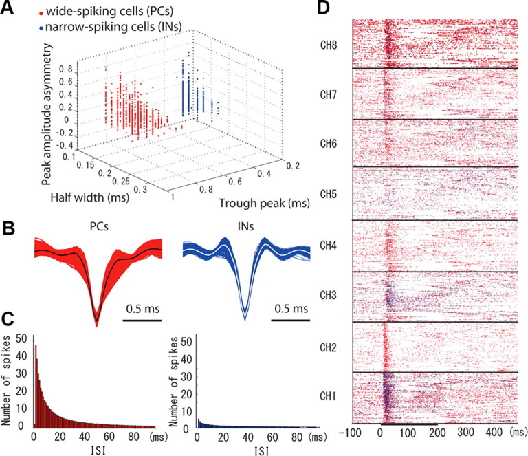
The classification of the neuron types for the population codifiers in one particular rat (001). A, The results from applying the SPC method (Quiroga et al., 2004) and the K-mean clustering show a clear distinction of two types of neurons underlying the population codifiers (red dot, wide-spiking PCs; blue dot, narrow-spiking INs). To estimate the peak amplitude asymmetry, half-width, and trough peak, the mean spiking waveforms of the identified neurons through the SPC method were pooled. The K-means method was used to evaluate clusters formation in the three-dimensional space defined by these parameters. B, Mean spiking waveform for each identified neuron (red curves, PCs; blue curves, INs). The grant averages of the PC and IN mean spiking waveforms for all neurons were overlapped using black and white curves, respectively. C, Histograms of the interspike interval (ISI) for each neuron during sound codification in this particular rat. These histograms revealed a key participation of the PCs in the sound codifying strategies in the A1. Based on the neuron classification, we were able to create electrode-based roster plots for the PCs and INs in each particular condition. D, Electrode-based roster plots for a particular condition (f_c, 8 kHz; f_m, 50 Hz; Amp, 70 dB) in rat 001.

Testing phase--amplitude couplings and their relation to MUA.

It was suggested previously that the spontaneous LFP oscillations are organized with the phases of the low-frequency bands modulating the amplitudes of the high-frequency bands in a sort of hierarchical structure. Such a phase–amplitude coupling (PAC) happens to occur in association with different brain functions, e.g., sensorial (Lakatos et al., 2005; Whittingstall and Logothetis, 2009), behavioral tasks (Canolty et al., 2006), and sleeping (Dalal et al., 2010; Le Van Quyen et al., 2010). Furthermore, increases in the MUA have been related to particular states of those variables exhibiting a PAC effect, henceforth called the PAC→MUA effect. For auditory tasks, the highest amplitudes θ frequency band oscillations in A1 occurred at a specific phase of the δ frequency band oscillations [i.e., θ-amplitude/δ-phase coupling (Lakatos et al., 2005)]. These authors also reported a similar γ-amplitude/θ-phase coupling and a clear phase-related modulation in the MUA for all frequency bands.

The alternating conditional expectation (ACE) algorithm (Wang and Murphy, 2004) provides us a method to verify relationships between independent and dependent variables without any a priori assumption about the underlying functions. An ACE regression model has the following general form:

where θ is a function of the dependent variable (response) Y, ϕ_i are functions of the independent variables (predictors) X_i(i = 1 …, p), and ε is the error term. The parameter α represents an arbitrary constant term. Therefore, the ACE regression model is robust and could be useful to study the existence of PAC→MUA effect for each cortical lamina from the MUA and CSD time-series data associated with our codifiers. For example, the particular model we are interested in testing is Y = X₁(X₂ − ϑ), which explicitly pointed out that MUA (Y) is maximal when the instantaneous CSD amplitude (X₁) of a particular frequency band is also at its maximum and, at the same time, the instantaneous CSD phase (X₂) of any other frequency band is 180° away from a given phase ϑ. This model can be written as an ACE regression model with the following particular form:

However, to validate the existence of the PAC→MUA effect, it is also necessary that functions θ and ϕ_i be represented by means of a minimal number of parameters in practice. The departure from complete spatial randomness in the Y − ϑ(Y) and X_i − ϕ_i(X_i) point maps could be used as a quantitative measure of the level of parameterization needed to represent functions θ and ϕ_i. Methods based on “second-order” (i.e., all point-to-point distances) and “first-order” (i.e., only mean interpoint distances) statistics have been developed for spatial point pattern analysis in geographical epidemiology (Gatrell et al., 1996). In this study, we used the Ripley's K-function with the edge correction, which constitutes one of the most useful functions for estimating the second-order statistics that gave rise to the data in the two-dimensional point pattern analysis (Ripley, 1977). The existence of the PAC→MUA effect was tested by applying the one-way ANOVA to the areas under the Ripley's K-function for two groups defined in terms of the used independent variables (group 1, the amplitudes of high-frequency oscillations X₁ and the phases of low-frequency oscillations X₂; group 2, the amplitudes of low-frequency oscillations X₁ and the phases of high-frequency oscillations X₂).

Results

We evaluated the accuracy of the 3-D probe insertion in A1 from information about the vessel distribution. For each experiment, the relative position of the 3-D probe and the vessels were obtained from both high-resolution photographs of the craniotomy area and the DiI-based vessel staining (Fig. 1B). From our estimation, the 3-D probe was successfully inserted inside A1 in the five rats.

Spatial aggregation/segregation of attribute codifiers

Based on the fact that we have colocalized shanks in each experiment with respect to the main canonical vessels in A1, we were able to differentiate the position of each codifier type (Fig. 6). We were looking for (1) the presence of sparse distributions, rather than topologically arranged dense networks, with high heterogeneity for the selective neuronal populations; and (2) any tendency in the organization of sound codifiers either in the tonotopic or in the iso-frequency axis.

Figure 6.

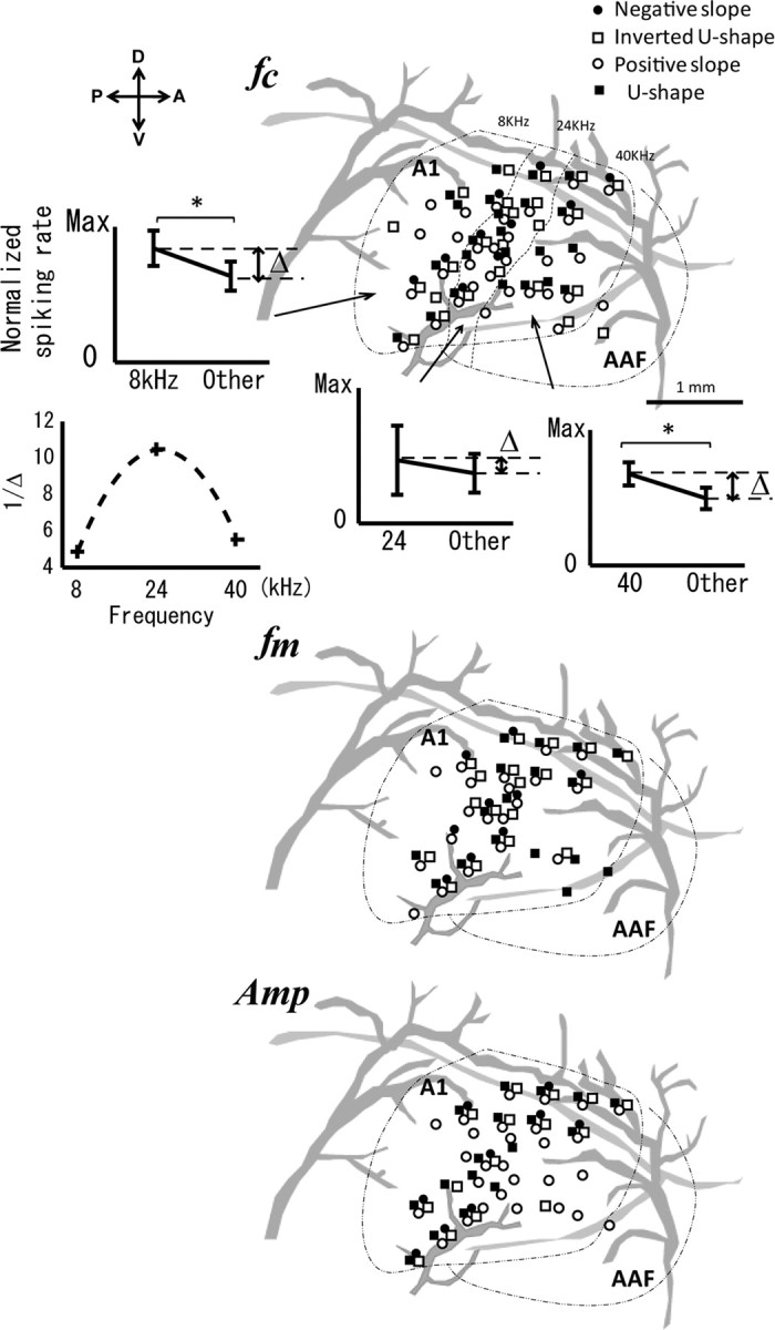
The distributions of the population codifiers in A1 for all rats. Top, Although the distributions of the carrier frequency codifiers in the A1 were heterogeneous, the spiking (inserted plots) rate showed an intrinsic tonotopical distribution (see below). The black dotted line delimited the A1 core region and the anterior auditory field (AAF); the large vessels are represented in gray. The actual locations of different types of codifiers are shown (blue diamonds, negative slope; orange diamonds, inverted U shape; green diamonds, positive slope; purple diamonds, U shape). The black dashed lines approximately delimited the regions in A1 corresponding to the three different threshold-based carrier frequencies (i.e., a coarse tonotopic map): 8, 24, and 40 kHz. The region-dependent population's susceptibility Δ was defined as the differences between the normalized/integrated spiking rate specific for each region (a particular carrier frequency) and that corresponding to the other two carrier frequencies. The inverse of the parameter Δ shows a bell-shaped dependency (i.e., a decrease in the population susceptibility for the midfrequency region) with the carrier frequency (f_c). This result is in agreement with the variations of the narrow (broad) bandwidth Q₁₀ (Q₄₀) along the anteroposterior axis of the A1 (Imaizumi and Schreiner, 2007). Middle and bottom, Distributions in A1 of the population codifiers of the modulation frequency and the amplitude, which were also heterogeneously distributed. Diagrams were created by coregistering the codifier's locations obtained for all rats. D, Dorsal; V, ventral; A, anterior; P, posterior; Max, maximum.

First, we found that all types of population codifiers for the carrier frequency f_c were distributed heterogeneously in A1 (Fig. 6, top). The most abundant type was the positive slope codifier, which may consist of neurons with high-pass tuning patterns similar to those reported in the past (Turner et al., 2005; Sakata and Harris, 2009). Second, to reproduce the classic tonotopic organization in the sense of neuronal populations, for each carrier frequency f_c, we calculated the mean of the spiking rate resulting from integrating the other two conditions (i.e., modulation frequency f_m and amplitude Amp). Consistent with previous studies (Doron et al., 2002; Rutkowski et al., 2003), we reproduced an obvious tonotopic organization in the rat A1 along the anteroposterior axis (Fig. 6, top subplots). This tonotopic organization was statistically significant for low (8 kHz) and high (40 kHz) carrier frequencies. However, it was hard to discriminate the 24 kHz neuronal responses in the midfrequency region of A1 from the population spiking. For each region of A1, we estimated the difference Δ between the population spiking rate for the characteristic frequency and the mean of that rate for the other two used frequencies. The introduced parameter Δ reflects the population's susceptibility in the region to its characteristic frequency. By plotting the fraction 1/Δ versus f_c (Fig. 6, top, bottom left subplot), we found a decrease in the population susceptibility for the midfrequency region along the anteroposterior axis. In our opinion, this is caused by the increase in Q₁₀ and Q₄₀ in this region of A1, as was recently reported for cats [Imaizumi and Schreiner (2007), their Fig. 2]. Large Q_10/40 values are associated with narrow bandwidths (i.e., neurons with high selectivity for the carrier frequency), hence a lower population susceptibility. However, our result is inconsistent with the increase in Q₁₀ toward the highest-frequency regions in A1, as was originally reported for rats [see Sally and Kelly (1988), their Fig. 9].

Figure 9.

The contribution of each neuron type to the population strategies of sound attribute codification in A1. The results of comparing the contributions of each neuron type to all sound attributes are shown (one-way ANOVA with multiple comparisons, *p < 0.05). In most cases, PCs are the neuron type with major contributions in the population codifying strategies. However, the contributions of INs, even though they are smaller than those of the PCs, must not be ignored. In particular, significant differences in the role of each neuron type for different sound attributes can be appreciated.

We found that population codifiers for both modulation frequency (Fig. 6, middle) and amplitude (Fig. 6, bottom) were heterogeneously distributed along the entire A1 core. Similar topological representations have been reported in previous studies for single neurons codifying the modulation frequency [rats (Kilgard and Merzenich, 1999), monkeys (Bendor and Wang, 2005, 2010)]. From our methodology, it was impossible to identify any particular signature of the segregation of monotonic (i.e., positive slope) and nonmonotonic (i.e., inverted U-shape) neuronal populations (Sutter and Schreiner, 1995; Recanzone et al., 2000; Linden and Schreiner, 2003).

Input/output functioning principles for the neuronal codifiers

We have evaluated the topological organizations of neuronal codifiers in A1 that were defined from a robust characterization of the population spiking rates. To understand the input/output functioning principles of these population codifiers, we will henceforth examine (1) perturbations in the CSD oscillatory laminar profiles and (2) CSD–spike relationships during both ongoing and auditory-evoked activity.

CSD oscillatory laminar profiles (spectral perturbations)

Figure 7A shows the grand average of the time-frequency difference map (left) for each layer in A1. We have highlighted three main periods (i.e., the prestimulus, the stimulus, and the poststimulus). We were mostly interested in evaluating sustained activity during both stimulus and poststimulus periods. To that end, we divided the stimulus period into two time windows of 100 ms each (i.e., P1 and P2). The time window P1 must reflect mainly stimulus onset effects. In a similar way, the poststimulus period was divided into two time windows of the same size (i.e., P3 and P4). The latter division aims both to ensure the same window size for the statistic analysis and to differentiate short- from long-lasting poststimulus effects. A magnification of a particular segment that includes periods P2–P4 (Fig. 7A, box delimited with a white dashed line) is shown on the right. The results of applying the Wilcoxon signed-rank tests (Bonferroni corrected p values, p < 0.05) to detect changes in the spectral content for all subwindows (i.e., P1–P4) at each layer are shown in Figure 7B. We applied the Kruskal–Wallis tests (**p < 0.01, *p < 0.05) with the Tukey's honestly significant difference criterion (i.e., the HSD method) to evaluate laminar differences (Fig. 7C).

Figure 7.

The layer-dependent perturbations in the CSD power spectral content in the stimulus and poststimulus periods. A, The grand average (i.e., pooled over the 384 codifiers) of the time-frequency difference map (right) are shown for the three layers (rows). To differentiate between sustained and stimulus (onset)-induced activities, the stimulus (horizontal black bar) period was divided into two time windows (P1 and P2). Both to ensure the same window size for the statistic analysis and to differentiate short- from long-lasting poststimulus effects, the poststimulus period was also divided into two time windows (P3 and P4). Magnifications of the time-frequency difference maps for the particular segments delimited with white dashed lines (left) are shown on the right. Sustained oscillatory activity in the γ_H (P2) and β (P3 and P4) frequency bands were highlighted in these magnifications. B, Results of applying the Wilcoxon signed-rank tests (Bonferroni corrected p values, p < 0.05) to detect stimulus-induced changes in the spectral content for time windows P1–P4 at each layer. C, Results of applying the Kruskal-Wallis tests (**p < 0.01; *p < 0.05) with the Tukey's honestly significant difference criterion (i.e., the HSD method) to evaluate laminar differences in the stimulus-induced spectral perturbations for all time windows P1–P4.

We found a transient broadband power increase (8–170 Hz) in all layers after the stimulus onset (i.e., P1 time window), with the low-frequency bands (i.e., δ, θ, α) having significantly higher power in the IG layer. In the P2 time window, we were able to detect a minor, but significant, increase in power for the γ_H frequency band at the SG layer that happened together with a reversion in the interlaminar power profile for the low-frequency bands (i.e., δ, θ, α). Such γ_H frequency band oscillatory activity remained up until the P3 time window. The poststimulus P3 and P4 time windows were both characterized by a global attenuation in the spectral content for the low-frequency bands with respect to the prestimulus period and a significant increase in power for the β-oscillations in all layers (with no significant differences among layers). In the P3 time window, there was a second reversion in the interlaminar power profile for the low-frequency bands with a partial recovery of power in the IG layer. In this time window, we could appreciate a significant increase in the power of the γ_L frequency band in all layers. Laminar differences in the power content for the low-frequency bands disappeared in the P4 time windows.

CSD–spike relationships (ongoing vs auditory-evoked activity)

Taking into account laminar features for single trials, we evaluate henceforth the instantaneous correlations between the amplitude/phase of CSD oscillations at each frequency band (i.e., δ, θ, α, β, γ_L, and γ_H) and the respective MUA. To that end, we performed a one-way ANOVA (p < 0.05) with multiple comparisons for every frequency band, pooling information about the single-trial correlations from all codifiers at each particular period and layer (Fig. 8A, interperiod differences, B, interlamina differences).

Figure 8.

The relationship between the MUA and the CSD amplitude. A, Correlation between the MUA and the CSD amplitude are shown for each layer (i.e., SG, G, and IG), frequency band (i.e., δ, θ, α, β, γ_L, and γ_H), and period (i.e., prestimulus, stimulus, and poststimulus). The statistical differences among different periods for each layer and frequency band are shown (ANOVA with multiple comparisons, *p < 0.05). B, To compare the dependency of these correlations along cortical layers, we applied the ANOVA with multiple comparisons (*p < 0.05) for the three frequency bands that showed highest correlations (i.e., β, γ_L, and γ_H). Corr. Coeff., Correlation coefficient.

The CSD amplitude and MUA correlations at all layers increased significantly during the stimulus period for the α, β, γ_L, and γ_H frequency bands. These two magnitudes were negatively correlated in all layers for the δ frequency band during both the prestimulus and poststimulus periods, but their correlation became positive during the stimulus period. For all layers, such a negative correlation was significantly higher in the prestimulus period. With respect to the prestimulus period, the correlation significantly decreased in all layers during the poststimulus period for the β, γ_L, and γ_H frequency bands (Fig. 8A). A similar decrease for the α frequency band was only observed in the G layer. For the θ frequency band, the correlation in both G and IG layers first increased significantly during the stimulus period and then decreased for the poststimulus period (Fig. 8A, middle and right).

As shown, CSD amplitudes for the β, γ_L, and γ_H frequency bands were highly correlated with MUA at all layers (Fig. 8B). However, we were able to detected interlaminar differences for each of these three frequency bands. The correlation in the β frequency band was higher in the IG layer during the stimulus and poststimulus periods. For the poststimulus period, this correlation in the SG was higher than in the G layer. During the stimulus period, the highest correlations for the γ_L frequency band were found in the IG layer, followed by the G and SG layers in a decreasing order. Such a high correlation in the IG layer for this particular frequency band dropped off in the poststimulus period. For the γ_H frequency band, the correlation was significantly higher in the SG layer for both the stimulus and poststimulus periods. In contrast to the other two frequency bands, there were significant differences in the laminar content of the correlation for the γ_H frequency band during the prestimulus period, with the largest values being in the SG layer.

From these results, we concluded that the temporal profile of MUA underlying attribute codification (i.e., during the stimulus period) is different at each layer with relatively slower (β and γ_L) dynamics at the IG layer and unquestionably faster dynamics (γ_H) at the SG layer. It has been pointed out that sensory-evoked activity propagates fast from layer IV to layers II/III and V (Sakata and Harris, 2009; Rothschild et al., 2010). These authors reported that small fractions in layer II/III, which are distributed sparsely, are activated in the preferable stimulus condition. From our data, we hypothesize that low (β–γ_L) and high (γ_H) dynamics in the postsynaptic potentials at the respective IG (sparse) and SG (dense) laminas might be associated with efficient inputs to the respective codifying neurons. The correlations between the CSD phase and MUA were very small. Hence, we did not perform a laminar structure analysis for the relationships between the CSD phase and the MUA (data not shown).

Laminar profiles for neuron types

We determined the contributions of each type of neuron, i.e., PCs and INs, to the population codification of sound attributes and their respective laminar profiles (tested using the one-way ANOVA with multiple comparisons, p < 0.05). Figure 9 shows the laminar distributions of the normalized spiking rates for both PCs and INs that were obtained using all neuronal codifiers. For all sound attributes, the contribution from PCs was not only more significant than from INs in the SG and IG layers, as expected, but, surprisingly, it was also more significant in the G layer. Sakata and Harris (2009) provided evidence for the contribution of L4 PCs in the codification of sound attributes in rats. In all layers, the contributions of PCs to the population codifiers were significantly larger for the attributes f_m and Amp. The activity of INs was small and about the same in the SG layer for all sound attributes. However, IN activation in the G and IG layers was not only a little bit higher but also showed interattribute differences. For example, INs in the IG layer were more active during the codification of the attribute Amp. In the G layer, activation of INs was only statistically distinguishable for attributes f_c and Amp. There is an interesting discussion by Sakata and Harris (2009) about the differentiated role played by these two types of neurons while processing sounds in A1. Our results are consistent with Sakata and Harris (2009), who suggested that the sensory-evoked spiking activity in A1 is mainly based on the activity of layer 2/3 and 5 PCs.

PAC→MUA effect in A1 for anesthetized rats

We tested the existence of the PAC→MUA effect for sound codification in anesthetized rats by applying the ACE regression analysis to the data corresponding to individual codifiers. For each layer and period, we performed such an analysis for amplitude and phase pairwise combinations (i.e., the independent variables) in all frequency bands. The MUA always constitutes the dependent variable. For all layers, periods, and amplitude–phase pairs, the mean (across codifiers) of the ACE correlation coefficients was between 0.7 and 0.8 (data not shown). Such a high correlation coefficient indicates a good predictability of the dependent variables based on the values of the independent variables by means of the estimated functions θ and ϕ_i.

Figure 10A (top) shows the results using a particular codifier of the ACE regression for the γ_H-amplitude and the δ-phase as the pair of independent variables. Figure 10A (bottom) shows the Ripley's K-functions for the corresponding normalized point distributions for functions θ and ϕ_i. In this study, to quantify the degree of parameterization of the ACE regression functions for each codifier and amplitude–phase pair, we used the average area under the Ripley's K-functions for the three corresponding normalized point maps. The areas under the Ripley's K-function for these representative point maps are given in Figure 10A. The higher this area is, the smaller the degree of randomness of the respective point map. Figure 10B (left) shows the average areas (grayscale matrix map) of the Ripley's K-functions of all possible combinations of amplitude and phase pairs for this particular codifier (positive slope, Amp), layer (SG), and period (prestimulus).

Figure 10.

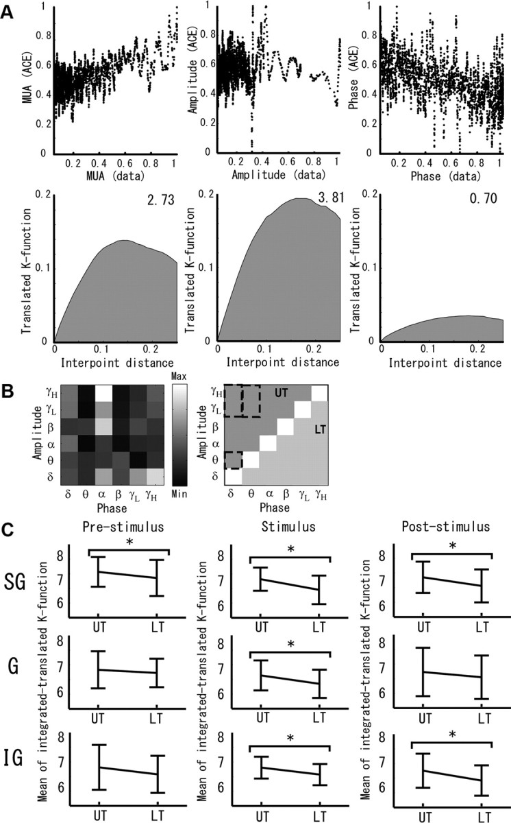
Evaluation of the PAC→MUA effect in the A1 of anesthetized rats. A, Data from a single codifier is used to exemplify the ACE regression analysis. Top, The plots represent the point maps for the dependent Y − ϑ(Y) (left, MUA) and the independent X_i − ϕ_i(X_i) (middle, CSD γ-amplitude; right, CSD δ-phase) variables for a particular layer and period. These point maps show no clear logarithmic forms as expected from the classical PAC→MUA effect (Eq. 2) in the visual cortex of monkeys for these particular combinations of independent variables (Whittingstall and Logothetis, 2009). Bottom, The plots show the results of estimating the Ripley's K-function with the edge correction to evaluate the degree of randomness in these point distributions. For a point map, the Ripley's K-function defines the dependency of the clusterization levels with the interpoint distances. Clearly, the point map with the highest function dimensionality/randomness (i.e., for the CSD δ-phase) has a smaller area under the Ripley's K-function (right). B, The areas under the Ripley's K-function estimated for all amplitude and phase pairwise combinations for this particular codifier are shown using a grayscale matrix map (left). High values in the upper triangle part of such a matrix indicates a low degree of randomness not only in the Y − ϑ(Y) point map but also in the ACE regression functions for the particular combinations of high-frequency CSD amplitude and low-frequency CSD phase (i.e., a PAC→MUA effect) for independent variables (group 1). PAC effects reported in the past for the sensory cortices in monkeys (Lakatos et al., 2005; Whittingstall and Logothetis, 2009) are highlighted with dashed boxes. C, The results of comparing (ANOVA, *p < 0.05) the upper and lower triangle parts of the matrices, estimated from 62 randomly selected codifiers, are shown for each layer and period. UT, Upper triangle; LT, lower triangle; Max, maximum; Min, minimum.

The hierarchical organization of the PAC→MUA effect with the phases of the low-frequency bands modulating the amplitudes of the high-frequency bands implies the upper triangle (UT) parts of the matrices in Figure 10B must be larger than the lower triangle (LT) parts. Figure 10C shows the respective means and SDs of the averaged UT and LT parts for the matrices estimated from 62 randomly selected codifiers. The content in the UT parts (group 1; see Materials and Methods) of these matrices were statistically significantly higher (p < 0.05) than that in their LT parts (group 2). It implies functions θ and ϕ_i resulting from the ACE regression analysis have lower dimensionalities for the amplitude (high-frequency oscillations)–phase (low-frequency oscillations) pairs. During ongoing activity (prestimulus period), such significant differences were observed only in the SG layer, which is in agreement with the laminar organization of PAC effect in A1 (Lakatos et al., 2005). However, the stimulus presentation induced a PAC→MUA effect in all cortical layers, probably related to the entrainment of the low-frequency oscillations to stimulus presentation (i.e., 1.6 s interstimulus interval → 0.6 Hz) (Lakatos et al., 2005). The PAC→MUA effect in the SG and IG layers (i.e., the endogenous processing layers) remained up until the poststimulus period. Therefore, MUA is mainly related to the CSD amplitudes for the β, γ_L, and γ_H frequency bands, holding clear relationships to the CSD phases at low-frequency bands.

Discussion

Here, we attempt to create a bridge between studies of sound processing in the A1 based on single-unit analysis and those that use population strategies. In particular, we investigated the topological segregations of sound attributes inside the A1 using coarse representations of the spiking sensitivity of different neuronal populations underlying an audio signal codification. To that end, we used a homemade, silicon-based 3-D probe. We defined four types of population codifiers, i.e., positive slope, negative slope, inverted U shape, and U shape. The distributions of these codifiers in A1 were heterogeneous at a large spatial scale. To understand the input/output dynamics of these codifiers, we explored both the CSD–spike relationships during ongoing/stimulus-related activity and the unit activity/oscillatory laminar profiles. We found that when codifying sound attributes, the MUA in the IG and SG laminas were correlated to the CSD amplitudes of the β-γ_L and the γ_H frequency bands, respectively. The relationships between MUA and the CSD amplitudes of these high-frequency oscillations were dependent of the CSD phase of the low-frequency oscillation, i.e., a global PAC→MUA effect. Nonphase-locked activity showed specific interlaminar profiles for each frequency band. These profiles additionally changed with time, as was evaluated using different periods relative to the stimulus onset/offset. After stimulus onset, long-lasting oscillatory activity in different frequency bands showed laminar specificities, with β and γ_H oscillations observed predominantly in the IG and SG layers, as was reported in vitro for the somatosensory cortex of rats (Roopun et al., 2006). Interestingly, spectral content in the low-frequency bands for all laminas fluctuated very much in these periods. The codification of sound attributes was mainly associated with the activity of PCs in all cortical laminas. INs were also involved, but to a minor degree. There was a clear laminar distinction in the relative role of these two neuron types for the codification of the sound attributes.

Interpreting the population codifiers

Neurons that might play an important role in codifying auditory signals have been identified by their particular responses (i.e., the spike rate) to variations of sound parameters. The most established auditory codifiers are associated with neurons that show FRA maps with tuning characteristics for one or two of these sound's attributes (e.g., monotonic V-shaped and nonmonotonic O-shaped FRA maps). FRA maps with multiple patterns have also been reported in the past. For example, Turner et al. (2005) showed some neurons with complex, intermediate, and high-threshold FRA maps in layer V of the rat A1, which is in agreement with the FRA maps latterly noted by Sakata and Harris (2009) for PCs and INs in other cortical layers of the rat A1. Neurons with separated subregions in their FRA maps, besides classical V-shaped tuning, have also been found (Gaese and Ostwald, 2003). The complexity of FRA maps in A1 is such that, based on a two-tailed split Gaussian model, Watkins and Barbour (2011) recently introduced a subclassification for neurons with monononic/nonmonotonic response curves (i.e., strong, weak, upper, and lower). This last study constitutes a step forward in the original classification used by Schreiner et al. (1992), who based the analysis of topological distributions for codifying neurons on five parameters (i.e., threshold, transition point, strongest response level, dynamic range, and monotonicity).

Identifying these types of neurons with electrophysiological techniques, and at the same time investigating their topological/laminar distributions and input/output working principles, is a highly challenging endeavor. Therefore, we defined sound codifiers based on the classical FRA maps for codifying neurons in the A1 and adapted them to the case of a coarse representation of the population spiking rates. The strategy we adopted was to use a simple definition that captures the activity of the predominant codifying networks in close proximity to the electrodes. There were few previous studies that defined similar types of coarse scales for the single neurons that codify these two sound attributes (Bizley et al., 2010; Watkins and Barbour, 2011).

Finally, the amplitude modulation of a pure tone or, alternatively, its periodicity constitutes the simplest example of time envelopes in a sound level. We did not focus our attention on neurons codifying the frequency modulation based on a temporal strategy but on those achieving it without delay through early variations in the levels of MUA. Using the population MUA for neuronal codifiers of the attribute f_m, we were able to determine the periodicity of a sound from its first repetitive cycles. We believe that such types of neurons, which quickly modify their spiking rates depending on variations in sound levels, must be crucial for survival and behavior.

Topological heterogeneity

The concept of “sparseness,” as defined by previous studies, originated from the fact that only a small fraction of neurons is required for sound codification, as observed in the time domain (Hromádka et al., 2008) and at a small spatial scale (Sakata and Harris, 2009; Harris et al., 2011). In this sense, a few preferable neurons seem to be enough to properly codify any sound attribute. For example, Smith and Lewicki (2006) reconstructed natural complex sounds from the spikes generated by a few neurons. In our study, the population codifiers of sound attributes were, in a large-scale sense, heterogeneously distributed and sparse in the rat A1 region (Rothschild et al., 2010). Our main results regarding spatial distributions of the underlying population codifiers, as well as their neuronal compositions and laminar profiles, were consistent with data reported in previous studies for different species, e.g., classical tonotopic organization in rats (Sally and Kelly, 1988; Doron et al., 2002; Rutkowski et al., 2003), the complex character of sound level representation in the A1 core in cats (Schreiner et al., 1992), the existence of a patchy organization for the suprathreshold neuronal activation in rats and guinea pigs (Bakin et al., 1996), the particular laminar profile for several neuronal types in rats (Wallace and Palmer, 2008; Sakata and Harris, 2009), and the uniform distribution of neurons sensitive to modulation frequency in rats/monkeys (Kilgard and Merzenich, 1999; Bendor and Wang, 2005, 2010).

These days, silicon-based probes that have excellent compatibility with brain tissues are built with microelectrodes for both voltage recording and current stimulation (Kipke et al., 2008). Therefore, our strategy for codifier selection and characterization is helpful, not only in reconstructing the neuronal encoders of sounds in A1, but also for recreating complex sound percepts through adequate stimulation (e.g., by prosthetic devices) of the neural tissue in close proximity to each population codifier (Deliano et al., 2009).

Spiking and postsynaptic activities: dynamic relationships

From observations in the A1 of monkeys, Lakatos et al. (2005) reported initially two hierarchically organized PAC effects (i.e., δ-phase/θ-amplitude and θ-phase/γ-amplitude couplings) that occurred in all layers during spontaneous activity, but that were greater in the SG layers. The latter result may be in agreement with the highest PAC→MUA effect reported in this study for the SG layer during the prestimulus period. However, in the study by Lakatos et al. (2005), phase-related modulation in the MUA was found to be larger in the G layer. These authors also demonstrated that the sensory-related CSD response and MUA depend on the phase of oscillatory activity in the δ frequency band at the stimulus onset and that such dependence showed a laminar profile. From our data, the global emergence of the PAC→MUA effect in all cortical layers during sensory stimulation may hold a direct relationship with the entrainment of ongoing oscillations in the δ frequency band during rhythmic stimulation. The PAC effect probably emerges mainly in experimental paradigms with high attention demand [e.g., θ-phase/γ-amplitude coupling in humans (Canolty et al., 2006); δ-phase/γ-amplitude coupling in monkeys (Whittingstall and Logothetis, 2009)] and it is totally attenuated during the anesthetized stage. However, in the past, evidence of PAC effects in anesthetized animals has also been found (Montemurro et al., 2008).

In different experimental protocols, the existence of time variations in the interlamina spectral contents at different locations in the A1 during periods of sound processing has previously been reported (Lakatos et al., 2005; Steinschneider et al., 2008). It has been suggested that such a laminar organization of the CSD oscillatory content might reflect the actual flow of information inside cortical columns (Oviedo et al., 2010) from different neuronal populations during both spontaneous and entrained activity (Atencio and Schreiner, 2010). Lakatos et al. (2005) found a laminar segregation in the amplitudes of the spontaneous oscillations, with higher powers in the δ–θ frequency bands for the SG layers and lower power in the γ frequency bands for the IG layers. The stimulus induced an increase in the power of the θ and γ frequency bands, but not in the power of the δ frequency band. The latter results are, to some extent, in agreement with findings in the current study for the neuronal codifiers in A1. We did not separate the effect of sources and sinks in each cortical layer; hence, our results are not comparable with those reported by Steinschneider et al. (2008).

Overall, our findings suggest that results based on single-unit analysis could be useful for tapering the strategies for population analysis, and vice versa.

References

- Atencio CA, Schreiner CE. Columnar connectivity and laminar processing in cat primary auditory cortex. PLoS One. 2010;5:e9521. doi: 10.1371/journal.pone.0009521. [DOI] [PMC free article] [PubMed] [Google Scholar]
- Bakin JS, Kwon MC, Susan AM, Weinberger NM, Frostig RD. Suprathreshold auditory cortex activation visualized by intrinsic signal optical imaging. Cereb Cortex. 1996;6:120–130. doi: 10.1093/cercor/6.2.120. [DOI] [PubMed] [Google Scholar]
- Bendor D, Wang X. The neuronal representation of pitch in primate auditory cortex. Nature. 2005;436:1161–1165. doi: 10.1038/nature03867. [DOI] [PMC free article] [PubMed] [Google Scholar]
- Bendor D, Wang X. Neural coding of periodicity in marmoset auditory cortex. J Neurophysiol. 2010;103:1809–1822. doi: 10.1152/jn.00281.2009. [DOI] [PMC free article] [PubMed] [Google Scholar]
- Bizley JK, Walker KMM, Silberman B, King AJ, Schnupp JWH. Interdependent encoding of pitch, timbre, and spatial location in auditory cortex. J Neurosci. 2009;29:2064–2075. doi: 10.1523/JNEUROSCI.4755-08.2009. [DOI] [PMC free article] [PubMed] [Google Scholar]
- Bizley JK, Walker KM, King AJ, Schnupp JW. Neural ensemble codes for stimulus periodicity in auditory cortex. J Neurosci. 2010;30:5078–5091. doi: 10.1523/JNEUROSCI.5475-09.2010. [DOI] [PMC free article] [PubMed] [Google Scholar]
- Canolty RT, Edwards E, Dalal SS, Soltani M, Nagarajan SS, Kirsch HE, Berger MS, Barabaro NM, Knight RT. High gamma power is phase-locked to theta oscillations in human neocortex. Science. 2006;313:1626–1628. doi: 10.1126/science.1128115. [DOI] [PMC free article] [PubMed] [Google Scholar]
- Dalal SS, Hamamé CM, Eichenlaub JB, Karim J. Intrinsic coupling between gamma oscillations, neuronal discharges, and slow cortical oscillations during human slow-wave sleep. J Neurosci. 2010;30:14285–14287. doi: 10.1523/JNEUROSCI.4275-10.2010. [DOI] [PMC free article] [PubMed] [Google Scholar]
- Deliano M, Scheich H, Ohl FW. Auditory cortical activity after intracortical microstimulation and its role for sensory processing and learning. J Neurosci. 2009;29:15898–15909. doi: 10.1523/JNEUROSCI.1949-09.2009. [DOI] [PMC free article] [PubMed] [Google Scholar]
- Doron NN, Ledoux JE, Semple MN. Redefining the tonotopic core of rat auditory cortex: physiological evidence for a posterior field. J Comp Neurol. 2002;453:345–360. doi: 10.1002/cne.10412. [DOI] [PubMed] [Google Scholar]
- Gaese BH, Ostwald J. Complexity and temporal dynamics of frequency coding in the awake rat auditory cortex. Eur J Neurosci. 2003;18:2638–2652. doi: 10.1046/j.1460-9568.2003.03007.x. [DOI] [PubMed] [Google Scholar]
- Games KD, Winer JA. Layer V in the rat auditory cortex: projections to the inferior colliculus and contralateral cortex. Hear Res. 1988;34:1–26. doi: 10.1016/0378-5955(88)90047-0. [DOI] [PubMed] [Google Scholar]
- Gatrell AC, Bailey TC, Diggle PJ, Rowlingson BS. Spatial point pattern analysis and its application in geographical epidemiology. Trans Inst Br Geogr. 1996;21:256–274. [Google Scholar]
- Goto T, Hatanaka R, Ogawa T, Sumiyoshi A, Riera J, Kawashima R. An evaluation of the conductivity profile in the barrel cortex of Wistar rats. J Neurophysiol. 2010;104:3388–3412. doi: 10.1152/jn.00122.2010. [DOI] [PubMed] [Google Scholar]
- Hackett TA, Barkat TR, O'Brien BMJ, Hensch TK, Polley DB. Linking topography to tonotopy in the mouse auditory thalamocortical circuit. J Neurosci. 2011;31:2983–2995. doi: 10.1523/JNEUROSCI.5333-10.2011. [DOI] [PMC free article] [PubMed] [Google Scholar]
- Harris KD, Bartho P, Chadderton P, Curto C, Rocha J, Hollender L, Itskov V, Luczak A, Marguet SL, Renart A, Sakata S. How do neurons work together? Lessons from auditory cortex. Hear Res. 2011;271:37–53. doi: 10.1016/j.heares.2010.06.006. [DOI] [PMC free article] [PubMed] [Google Scholar]
- Hromádka T, Deweese MR, Zador AM. Sparse representation of sounds in the unanesthetized auditory cortex. PLoS Biol. 2008;6:e16. doi: 10.1371/journal.pbio.0060016. [DOI] [PMC free article] [PubMed] [Google Scholar]
- Imaizumi K, Schreiner CE. Spatial interaction between spectral integration and frequency gradient in primary auditory cortex. J Neurophysiol. 2007;98:2933–2942. doi: 10.1152/jn.00511.2007. [DOI] [PubMed] [Google Scholar]
- Kilgard MP, Merzenich MM. Distributed representation of spectral and temporal information in rat primary auditory cortex. Hear Res. 1999;134:16–28. doi: 10.1016/s0378-5955(99)00061-1. [DOI] [PMC free article] [PubMed] [Google Scholar]
- Kipke DR, Shain W, Buzsáki G, Fetz E, Henderson JM, Hetke JF, Schalk G. Advanced neurotechnologies for chronic neural interfaces: new horizons and clinical opportunities. J Neurosci. 2008;28:11830–11838. doi: 10.1523/JNEUROSCI.3879-08.2008. [DOI] [PMC free article] [PubMed] [Google Scholar]
- Lakatos P, Shah AS, Knuth KH, Ulbert I, Karmos G, Schroeder CE. An oscillatory hierarchy controlling neuronal excitability and stimulus processing in the auditory cortex. J Neurophysiol. 2005;94:1904–1911. doi: 10.1152/jn.00263.2005. [DOI] [PubMed] [Google Scholar]
- Lakatos P, Chen C-M, O'Connell MN, Mills A, Schroeder CE. Neuronal oscillations and multisensory interaction in primary auditory cortex. Neuron. 2007;53:279–292. doi: 10.1016/j.neuron.2006.12.011. [DOI] [PMC free article] [PubMed] [Google Scholar]
- Langner G, Dinse HR, Godde B. A map of periodicity orthogonal to frequency representation in the cat auditory cortex. Front Integr Neurosci. 2009;3:27. doi: 10.3389/neuro.07.027.2009. [DOI] [PMC free article] [PubMed] [Google Scholar]
- Le Van Quyen M, Staba R, Bragin A, Dickson C, Valderrama M, Fried I, Engel J. Large-scale microelectrode recordings of high-frequency gamma oscillations in human cortex during sleep. J Neurosci. 2010;30:7770–7782. doi: 10.1523/JNEUROSCI.5049-09.2010. [DOI] [PMC free article] [PubMed] [Google Scholar]
- Li Y, Song Y, Zhao L, Gaidosh G, Laties AM, Wen R. Direct labeling and visualization of blood vessels with lipophilic carbocyanine dye DiI. Nat Protoc. 2008;3:1703–1708. doi: 10.1038/nprot.2008.172. [DOI] [PMC free article] [PubMed] [Google Scholar]
- Linden JF, Schreiner C. Columnar transformations in auditory cortex? A comparison to visual and somatosensory cortices. Cereb Cortex. 2003;13:83–89. doi: 10.1093/cercor/13.1.83. [DOI] [PubMed] [Google Scholar]
- Montemurro MA, Rasch MJ, Murayama Y, Logothetis NK, Panzeri S. Phase-of-firing coding of natural visual stimuli in primary visual cortex. Curr Biol. 2008;18:375–380. doi: 10.1016/j.cub.2008.02.023. [DOI] [PubMed] [Google Scholar]
- O'Connell MN, Falchier A, McGinnis T, Schroeder CE, Lakatos P. Dual mechanism of neuronal ensemble inhibition in primary auditory cortex. Neuron. 2011;69:805–817. doi: 10.1016/j.neuron.2011.01.012. [DOI] [PMC free article] [PubMed] [Google Scholar]
- Oviedo HV, Bureau I, Svoboda K, Zador AM. The functional asymmetry of auditory cortex is reflected in the organization of local cortical circuits. Nat Neurosci. 2010;13:1413–1420. doi: 10.1038/nn.2659. [DOI] [PMC free article] [PubMed] [Google Scholar]
- Paxinos G, Watson C. The rat brain in stereotaxic coordinates. Ed 6. Burlington, MA: Academic; 2007. [DOI] [PubMed] [Google Scholar]
- Pettersen KH, Devor A, Ulbert I, Dale AM, Einevoll GT. Current-source density estimation based on inversion of electrostatic forward solution: effects of finite extent of neuronal activity and conductivity discontinuities. J Neurosci Methods. 2006;154:116–133. doi: 10.1016/j.jneumeth.2005.12.005. [DOI] [PubMed] [Google Scholar]
- Quiroga RQ, Nadasdy Z, Ben-Shaul Y. Unsupervised spike detection and sorting with wavelets and superparamagnetic clustering. Neural Comput. 2004;16:1661–1687. doi: 10.1162/089976604774201631. [DOI] [PubMed] [Google Scholar]
- Rasch MJ, Schuch K, Logothetis NK, Maass W. Statistical comparison of spike responses to natural stimuli in monkey area V1 with simulated responses of a detailed laminar network model for a patch of V1. J Neurophysiol. 2011;105:757–778. doi: 10.1152/jn.00845.2009. [DOI] [PMC free article] [PubMed] [Google Scholar]
- Ray S, Maunsell JHR. Different origins of gamma rhythm and high-gamma activity in Macaque visual cortex. PLoS Biol. 2011;9:e1000610. doi: 10.1371/journal.pbio.1000610. [DOI] [PMC free article] [PubMed] [Google Scholar]
- Recanzone GH, Guard DR, Phan ML. Frequency and intensity response properties of single neurons in the auditory cortex of the behaving macaque monkeys. J Neurophysiol. 2000;83:2315–2331. doi: 10.1152/jn.2000.83.4.2315. [DOI] [PubMed] [Google Scholar]
- Riera J, Ogawa T, Hatanaka R, Goto T, Sumiyoshi A, Kadji HE, Nakauchi S, Kawashima R. Concurrent observations of astrocytic Ca2+ activity and multisite extracellular potentials from an intact cerebral cortex. J Biophotonics. 2010;3:147–160. doi: 10.1002/jbio.200910036. [DOI] [PubMed] [Google Scholar]
- Ripley BD. Modelling spatial patterns. J R Stat Soc B. 1977;39:172–212. [Google Scholar]
- Roopun AK, Middleton SJ, Cunningham MO, LeBeau FEN, Bibbig A, Whittington M, Traub RD. A beta2-frequency (20–30 Hz) oscillation in nonsynaptic networks of somatosensory cortex. Proc Natl Acad Sci U S A. 2006;103:15646–15650. doi: 10.1073/pnas.0607443103. [DOI] [PMC free article] [PubMed] [Google Scholar]
- Rothschild G, Nelken I, Mizrahi A. Functional organization and population dynamics in the mouse primary auditory cortex. Nat Neurosci. 2010;13:353–360. doi: 10.1038/nn.2484. [DOI] [PubMed] [Google Scholar]
- Rutkowski RG, Miasnikov AA, Weinberger NM. Characterisation of multiple physiological fields within the anatomical core of rat auditory cortex. Hear Res. 2003;181:116–130. doi: 10.1016/s0378-5955(03)00182-5. [DOI] [PubMed] [Google Scholar]
- Sadagopan S, Wang X. Level invariant representation of sounds by populations of neurons in primary auditory cortex. J Neurosci. 2008;28:3415–3426. doi: 10.1523/JNEUROSCI.2743-07.2008. [DOI] [PMC free article] [PubMed] [Google Scholar]
- Sakata S, Harris KD. Laminar structure of spontaneous and sensory-evoked population activity in auditory cortex. Neuron. 2009;64:404–418. doi: 10.1016/j.neuron.2009.09.020. [DOI] [PMC free article] [PubMed] [Google Scholar]
- Sally SL, Kelly JB. Organization of auditory cortex in the albino rat: sound frequency. J Neurophysiol. 1988;59:1627–1638. doi: 10.1152/jn.1988.59.5.1627. [DOI] [PubMed] [Google Scholar]
- Schreiner CE, Mendelson JR, Sutter ML. Functional topography of cat primary auditory cortex representation of tone intensity. Exp Brain Res. 1992;92:105–122. doi: 10.1007/BF00230388. [DOI] [PubMed] [Google Scholar]
- Schreiner CE, Read HL, Sutter ML. Modular organization of frequency integration in primary auditory cortex. Annu Rev Neurosci. 2000;23:501–529. doi: 10.1146/annurev.neuro.23.1.501. [DOI] [PubMed] [Google Scholar]
- Schulze H, Hess A, Ohl FW, Scheich H. Superposition of the horseshoe-like periodicity and linear tonotopic maps in auditory cortex of the Mongolian gerbil. Eur J Neurosci. 2002;12:1077–1084. doi: 10.1046/j.1460-9568.2002.01935.x. [DOI] [PubMed] [Google Scholar]
- Smith EC, Lewicki MS. Efficient auditory coding. Nature. 2006;439:978–982. doi: 10.1038/nature04485. [DOI] [PubMed] [Google Scholar]
- Steinschneider M, Fishman YI, Arezzo JC. Spectrotemporal analysis of evoked and induced electroencephalographic responses in primary auditory cortex (A1) of the awake monkey. Cereb Cortex. 2008;18:610–625. doi: 10.1093/cercor/bhm094. [DOI] [PubMed] [Google Scholar]
- Sutter ML, Schreiner CE. Topography of intensity tuning in cat primary auditory cortex: single-neuron versus multiple-neuron recordings. J Neurophysiol. 1995;73:190–204. doi: 10.1152/jn.1995.73.1.190. [DOI] [PubMed] [Google Scholar]
- Turner JG, Hughes LF, Caspary DM. Divergent response properties of layer-V neurons in rat primary auditory cortex. Hear Res. 2005;202:129–140. doi: 10.1016/j.heares.2004.09.011. [DOI] [PubMed] [Google Scholar]
- Wallace MN, Palmer AR. Laminar differences in the response properties of cells in the primary auditory cortex. Exp Brain Res. 2008;184:179–191. doi: 10.1007/s00221-007-1092-z. [DOI] [PubMed] [Google Scholar]
- Wang D, Murphy M. Estimating optimal transformations for multiple regression using the ACE algorithm. J Data Sci. 2004;2:329–346. [Google Scholar]
- Watkins PV, Barbour DL. Level-tuned neurons in primary auditory cortex adapt differently to loud versus soft sounds. Cereb Cortex. 2011;21:178–190. doi: 10.1093/cercor/bhq079. [DOI] [PMC free article] [PubMed] [Google Scholar]
- Whittingstall K, Logothetis NK. Frequency-band coupling in surface EEG reflects spiking activity in monkey visual cortex. Neuron. 2009;64:281–289. doi: 10.1016/j.neuron.2009.08.016. [DOI] [PubMed] [Google Scholar]
- Woolsey CN, Walzl EM. Topical projection of nerve fibers from local regions of the cochlea to the cerebral cortex of the cat. Bull Johns Hopkins Hosp. 1942;71:315–344. [Google Scholar]