Computation of Interaural Time Difference in the Owl's Coincidence Detector Neurons

Abstract

Both the mammalian and avian auditory systems localize sound sources by computing the interaural time difference (ITD) with submillisecond accuracy. The neural circuits for this computation in birds consist of axonal delay lines and coincidence detector neurons. Here, we report the first in vivo intracellular recordings from coincidence detectors in the nucleus laminaris of barn owls. Binaural tonal stimuli induced sustained depolarizations (DC) and oscillating potentials whose waveforms reflected the stimulus. The amplitude of this sound analog potential (SAP) varied with ITD, whereas DC potentials did not. The amplitude of the SAP was correlated with firing rate in a linear fashion. Spike shape, synaptic noise, the amplitude of SAP, and responsiveness to current pulses differed between cells at different frequencies, suggesting an optimization strategy for sensing sound signals in neurons tuned to different frequencies.

Introduction

Many animals use both ears to determine the direction of sound sources. The arrival time difference of sound between the two ears [interaural time difference (ITD)] is a major cue for localization in the horizontal direction (Konishi, 1993), and how ITDs are computed in the brain is of general interest (for review, see Grothe et al., 2010). The Jeffress model of sound localization uses axonal delay lines and coincidence detector neurons to encode ITDs (Jeffress, 1948). In the avian auditory system, axonal delay lines from the cochlear nucleus magnocellularis (NM) synapse on coincidence detector neurons in the nucleus laminaris (NL) (Carr and Konishi, 1990). Although the existence of delay lines in the mammalian brainstem is controversial (Grothe et al., 2010), coincidence detection is regarded as universally significant. Furthermore, the cellular mechanisms underlying coincidence detection in the auditory systems of birds and mammals have long been a subject of discussion and modeling because of their exceptional temporal precision (Gerstner et al., 1996; Agmon-Snir et al., 1998; Cook et al., 2003; Grau-Serrat et al., 2003; Kuba et al., 2006; Ashida et al., 2007).

Just how precise are auditory coincidence detectors? In owls, NL neurons change their firing rates with changes in ITD of <10 μs (Carr and Konishi, 1990; Peña et al., 1996), far below the spike duration of the neurons (e.g., ∼1 ms). The data used for modeling these coincidence detection processes have so far come from in vitro studies in the chick's NL (Reyes et al., 1996; Funabiki et al., 1998; Kuba et al., 2005, 2006; Slee et al., 2010), extracellular studies of the barn owl's NL neurons (Carr and Konishi, 1990; Peña et al., 1996; Fischer et al., 2008), and the owl's behavioral performance (Knudsen et al., 1979). Specialized cellular mechanisms, including extraordinary fast glutamate receptors (Reyes et al., 1996; Trussell, 1999; Kuba et al., 2005), low threshold-activated potassium conductance (KLVA) (Reyes et al., 1996), and remote spike initiation (Carr and Boudreau, 1993b; Kuba et al., 2006; Ashida et al., 2007), have been discussed as important elements of this extraordinary precise coincidence detection. Information regarding the subthreshold responses of NL neurons to real sound in vivo, however, has been lacking.

We designed coaxial glass electrodes that allowed us to obtain in vivo intracellular recordings in the owl's NL. Using this technique, we were able to record the synaptic input to these cells during sound stimulation and measure their input–output properties. Here, we show that the postsynaptic response of the NL cell is an analog waveform that closely resembles the sinusoidal stimuli and that its amplitude changes with ITD, which, in turn, drives the neuron to generate spikes.

Materials and Methods

Animals and surgery

Data were obtained from 16 adult barn owls (Tyto alba) of both sexes. Detailed descriptions of the surgery are available (Peña et al., 1996, 2001). In brief, owls were anesthetized with an intramuscular injection of ketamine hydrochloride (25 mg/kg) and diazepam (1.3 mg/kg). Additional ketamine injections were made as necessary. We tried recording from the caudal third of NL where cell density is higher than other regions (Carr and Boudreau, 1993a). For this purpose, we adjusted the angle of electrode in the coronal plane (see Fig. 1Ad). After experiments, the hole for electrode insertion was covered with dental cement and the skin incision was closed. Antibiotic and a local anesthetic in sterile solution were applied to the wound. Owls were returned to their individual cages and monitored for their recovery. The protocol for this study followed the National Institutes of Health Guide for the Care and Use of Laboratory Animals and was approved by the Animal Care and Use Committee of the California Institute of Technology.

Figure 1.

In vivo intracellular recording in NL cells using a coaxial glass electrode. A, a, Schematic drawing of a coaxial glass electrode advanced by two motors. A plastic T-tube and small silicon tubes used for pressure control were not drawn for simplicity. b, A photograph of two glass electrodes before inserting inner capillary into the outer one. Although a plastic T-tube was prepared for both inner and outer electrode, we only used one for the outer capillary to apply pressure. c, A photograph of the electrode tip after protruding the inner tip from the outer one. One large division on the scale beside the electrode corresponds to ∼20 μm. d, A photograph of brain slice at the AP level where recording was performed. We adjusted the angle of insertion of electrodes in the coronal plane to access the caudal third of NL with minimal craniotomy. Two broken lines indicate examples of the electrode path passing through the cerebellum. Scale bar, 2 mm. B, a, Current trace. Short 0.3 nA pulses were delivered to monitor the electrode and input resistance of the cell. b, Voltage changes during penetration. Tonal stimuli (3.9 kHz; 40 dB SPL; 60 ms) were delivered at regular intervals (bars). c, Spectrogram of voltage traces. d, Expanded trace of intracellular recording at the onset of tonal stimuli. C, Voltage traces with current injection. Tonal stimuli (3.4 kHz; 40 dB SPL; binaural) were delivered (bar) and spikes (gray) were detected by thresholding and removed from the analysis of SAP amplitude. Currents applied (in nanoamperes) are shown in parentheses. D, Membrane voltage data plotted against the phase angle of tones. The bold line is a fitted sine function. The amplitude of the SAP was defined as a peak-to-peak value of the fitted curve. E, An example of interspike interval histogram confirming an isolation of spikes.

Sound stimulation

All the experiments were performed in a double-walled acoustic chamber (Industrial Acoustic Company). An earphone assembly consisting of a Knowles 1914 receiver, a Knowles 1743 damping device, and a Knowles 1319 microphone (Knowles Electronics) delivered sound stimuli. These components are encased in an aluminum cylinder that fits into the owl's ear canal. The gaps between the cylinder and the ear canal were filled with silicon impression material (Gold Velvet II; Earmold and Research Laboratory). At the beginning of each experimental session, both earphone assemblies were automatically calibrated for sound pressure level (SPL) and phase. The computer was programmed to equalize SPL and phase for all frequencies within the frequency range relevant to the experiment. The stimuli consisted of tones and noise bursts of 60–100 ms in duration with a 3 ms rise–fall time, delivered one to two per second. The average binaural intensity of the sound stimulus was set to 40 dB SPL, unless otherwise mentioned. ITD was varied in steps of either 1/10th of the period for tonal stimuli or 30 μs. Firing rate and membrane potential changes as a function of ITD were typically measured for three repetitions of each stimulus.

As in previous studies (Carr and Konishi, 1990), and because the duration of recordings using sharp electrode did not allow for more precise measurements, the best frequency (BF) of each neuron was estimated with the aid of an audio monitor, by determining the stimulus frequency that elicited the strongest response. These BF measurements were confirmed by measuring the periodicity of ITD tuning curves collected using broadband noise. It has been shown that the period of broadband ITD curves shows strong correlation with the best frequency of the cell (Peña et al., 2001).

Electrophysiological recordings

Coaxial glass electrodes have been used to reduce the stray capacitance of the microelectrode for better voltage clamp (Schwartz and House, 1970; Sachs and McGarrigle, 1980). We adapted this configuration to obtain intracellular recording from NL neurons in vivo. This configuration allowed us to reach NL, which lies at a depth of ∼10 mm below the cerebellum, with sharp electrodes. The system consisted of a microelectrode [1B100F-4; outer diameter (o.d.), 1.0 mm; inner diameter (i.d.), 0.58 mm; WPI] inserted into a patch electrode-type capillary (PG52165-4; o.d., 1.65 mm; i.d., 1.1 mm; WPI; see Fig. 1Aa). The outer capillary protected the tip of the microelectrode during penetration. The tip of the outer electrode was filled with a small amount of oil (Zeiss immersion oil) to reduce the capacitance of the electrode and also to help in preventing the CSF from filling the empty space between the capillaries. Also, for the same reason, we applied a positive pressure to the outer capillary through a plastic T-tube connected to the outer capillary (see Fig. 1Ab). The inner electrode was filled with 3 m potassium acetate. We used two close-loop motor actuators: motor 1 and controller 1 (850G and ESP300), and motor 2 and controller 2 (850B-2 and PMC100; Newport; see Fig. 1Aa). The motor 1 advanced both the outer and inner capillaries and the motor 2 advanced only the inner one (see Fig. 1Aa). Before insertion into the brain, the inner electrode was inserted into the outer electrode until the distance between the two electrode tips was ∼300 μm under microscope (Unitron Toolmaker's microscope).

Using the motor 1, we drove both electrodes through the cerebellum to a depth of 7–8 mm, where we began to advance the inner microelectrode using the motor 2. The emergence of the inner electrode out of the outer electrode was noticed by monitoring both the DC potential and the electrode resistance. After the inner tip emerged, we advanced the inner electrode further up to ∼60 μm (see Fig. 1Ac). Too much protrusion would break the outer capillary. Subsequently, the motor 1 only was used to advance inner and outer electrodes together to obtain intracellular recordings in NL. High-impedance microelectrodes (>80 MΩ) were required to obtain stable intracellular recordings from NL cells. Therefore, we restricted applied currents to a range in which the microelectrode does not show much rectification (±1 to ±2 nA) when measuring changes in membrane potentials by current injection.

Voltage and current data were recorded with a Neurodata IR-183 (Cygnus Technology) or an Axoclamp 2A amplifier in bridge mode (Molecular Devices), and were stored on disk (through an AD converter; TDT system 2; Tucker-Davis Technologies; sampling frequency, 48 kHz) and tape (through a PCM encoder; Neurodata DR-484; Cygnus Technology; sampling frequency, 44.1 kHz). The data from current inputs and voltage outputs around penetration such as the one shown in Figure 1B were stored on tape.

We applied short current pulses (0.2–0.3 nA, 15–30 ms) periodically to monitor electrode and/or membrane resistance (see Fig. 1Ba). Small negative holding currents (0.2–0.4 nA) were used to facilitate penetration and help stabilize the membrane potential after penetration. The DC-potential drop at penetration (see Fig. 1Bb) was calculated after removing the effect of changes in electrode resistance occurring upon cell penetration. Resting potentials were measured without holding current. We used both DC drops and resting potentials to judge whether or not recordings were intracellular. Data from cells with resting potential lower than −50 mV, and DC drop >15 mV (determined by comparing data from putative axonal recording of NM and NL cells) were used for further analyses (mean resting potential, −58 ± 17 mV; mean DC drop, 33 ± 13 mV; n = 35).

The input resistances of NL cells, calculated from the change in membrane potential induced by small negative currents (around −0.3 nA) applied at resting potential, was low (10.4 ± 8.2 MΩ) and sometimes <5 MΩ for positive current steps. All the statistical results are shown in terms of mean ± SD. When analyzing correlation, we used Pearson's product-moment correlation in case the variables showed normal distribution (Kolmogorov–Smirnov test, p > 0.05). Otherwise, Spearman's rank correlation coefficient was used. When Pearson's product-moment correlation was used, we added a regression line in the corresponding figures.

Spike analysis

All the data were analyzed with custom-written MATLAB scripts (version 6.5R13; MathWorks). Spikes were analyzed as follows: First, voltage traces were bandpass filtered (30–3000 Hz), and spikes were detected by visually adjusting the threshold. In determining this threshold, care was taken so that both spontaneous and sound-induced spikes were detected (see Figs. 1Bb,C, 5A). We discriminated spikes from large EPSPs by checking the presence of refractory period in the interspike interval histogram (an example was shown in Fig. 1E) and increase in event rate by injecting depolarizing currents (see Figs. 1C, 6A). The program filed the spike timings and cut out the corresponding spike waveforms from original (non-bandpass-filtered) voltage traces. Next, spontaneous spikes (spikes occurring when neither sound nor current stimuli were applied) were collected and averaged over 10 events or more. This averaged spike waveform was used to determine the spike duration (i.e., when potential returns to the baseline level, ∼0.9 ms). We used this duration in analyzing compound potential response against tonal stimuli (see next section). The height and the width at half-amplitude of spontaneous spikes were also measured.

Figure 5.

Voltage traces and spike analyses of different BF NL cells. A, Voltage traces from three NL cells with different BFs. Tonal stimuli at BF were delivered during periods indicated by a bold bar. a, BF = 3.9 kHz. b, BF = 2.5 kHz. c, BF = 0.9 kHz. Note that spontaneous spike shapes are considerably different among these cells. B, Spike height plotted with respect to the BF of the cell. C, Spike width at one-half the peak amplitude (spike half-width) plotted with respect to the BF of the cell.

Figure 6.

Biophysical parameters and the best frequency of the cell. A, Examples of membrane potential traces in response to small positive currents. Two voltage responses against a current pulse (0.3 nA; duration, 20–30 ms) were shown for each cell with different BF. Capacitative artifacts are retouched for clarity. Calibration: 10 mV, 10 ms. B, Spike rate increase with 0.3 nA short pulse plotted with respect to BF of the cell. C, SDs of resting membrane potentials plotted with respect to BF of the cell.

Analysis of sound analog potential

Tonal stimuli induced periodic membrane-potential oscillations that closely resembled the stimulus waveform (see Results). These oscillations will be referred to as “sound analog potential” (SAP). To analyze SAPs, the times when spikes occurred (as determined in spike analysis; see Fig. 1C, gray) were first removed from analysis. The residual voltage data points during tonal stimuli (see Fig. 1C, black and under bold line) were plotted against the phase angle of the stimulus tones (see Fig. 1D). We fitted these points with a sinusoidal function: y = (A_SAP/2) · sin(θ) + DC, with θ being the phase of the stimulus tone. We used the value of A_SAP as the amplitude of SAPs (peak-to-peak value of the fitted curve) and the difference between averaged membrane potential 5–15 ms before sound stimuli (when no spikes were observed) and this DC value as a sound-evoked DC shift.

The change in SAP amplitude as a function of ITD was fitted to a cosine function: y = |H · cos(πf_s *ITD + θ₀)|, where H is the amplitude, f_s is the sound frequency, and θ₀ is the phase shift. The value of H was used as the maximal SAP induced by changing ITD.

In the analysis of SAP changes before and directly after penetration, we did not remove the times when spikes occurred, because spike amplitude and shape changed largely at the time of penetration. Instead, we measured changes in the spectral power corresponding to the stimulus frequency. The spectral power of spikes was mostly <1.5 kHz (see Figs. 1Bc, 2C) and thus did not greatly affect the analysis in the majority of cells recorded.

Figure 2.

ITD-dependent changes in membrane potential in high-frequency NL neuron. A, ITD was varied for a tone burst stimulus (3.9 kHz; 60 ms duration; bar above traces). a, Most favorable ITD (192 μs). b, An intermediate ITD (128 μs). c, Least favorable ITD (64 μs). B, Expanded traces from A (Aa, short bar below trace). C, Spectral analysis of membrane potentials shown in A. D, Spike rates plotted against ITD. The solid line marks a fitted sine curve (also in F and Fig. 3D,F). The asterisk (*) shows the spontaneous spike rate (also in E–H and Fig. 3D–H). E, SAP amplitude plotted against ITD. The solid line is a fit by an absolute cosine function. F, DC shift evoked by sound plotted against ITD. The horizontal axis is shared with D and E. G, Spike rate plotted against SAP amplitude. The asterisks indicate spontaneous firing rate. Also in H and Figure 3, G and H. H, Spike rate plotted with respect to DC shift.

Extracellular recordings

Using the same electrodes, it was also possible to record NL neurons extracellularly (n = 102). Unlike the intracellular recordings, the DC drop at the start of the unit recording was minimal (−1.4 ± 8.3 mV; n = 70). Field potentials, which also followed the waveform of sound stimuli (“neurophonic”), were also recorded on these voltage traces. Unlike the intracellular recordings, the neurophonic amplitude did not increase much at the beginning (1.2 ± 0.4; n = 50). Interestingly, extracellular spikes were rarely observed before penetration in intracellular recordings (see Fig. 1Bb), whereas penetration of membrane was never obtained when large (e.g., >2 mV) extracellular spikes are observed (n = 70), suggesting that extracellular recordings may have originated from NL axons.

Modeling

Synaptic input from NM to NL.

The modeling procedure has been described in detail (Ashida et al., 2007). Briefly, we calculated phase-locked synaptic inputs from ipsilateral and contralateral NM fibers into the NL neuron using known physiological data from owls and chicks (Table 1). The firing probability, which changes periodically with the stimulus frequency, was described by the von Mises distribution with a given vector strength (VS). Excitatory postsynaptic conductances (EPSCs) induced by each presynaptic NM spike were modeled by an α function f(t) = (At/τ) exp(1 − t/τ). The half-peak width W of the α function is linear to the time scale τ; namely, W = kτ, where the proportionality constant k = 2.446. In our simulation, W was set to 0.1 ms, unless otherwise noted. The peak height of the α function f(τ) = A was determined to be 2.0 nS (without sound) or 1.3 nS (with sound) so as to reproduce the AC amplitudes and the DC shifts observed in experiments. The 35% reduction (2.0 to 1.3 nS) in the EPSC amplitude by sound stimulus (see Results) may correspond to synaptic depression (Kuba et al., 2002; Cook et al., 2003) and/or shunting effects of inhibitory inputs to NL (Funabiki et al., 1998; Yang et al., 1999). In simulations in which the number of the half-peak width W of the EPSC was altered (see Fig. 7C,D), EPSC height A was readjusted to conserve the total conductance.

Table 1.

Model parameters used for synaptic input in NL

Parameter	Value	Reference
EPSC half-peak width	0.1 ms	Kuba et al. (2005, 2006): chick (adjusted to match experiment)
EPSC amplitude (spontaneous)	2.0 nS	(Adjusted to match experiment)
EPSC amplitude (with sound)	1.3 nS	(Adjusted to match experiment)
Convergence number of NM fibers	150 (each side)	Carr and Boudreau (1993a): owl
NM firing rate (spontaneous)	220 Hz	Köppl (1997a): owl
NM firing rate (with sound)	500 Hz	Peña et al. (1996): owl
NM vector strength	0.6	Köppl (1997b): owl

This table summarizes the parameters used for modeling the synaptic input between NM and NL. Relevant references are also shown. The half-peak width and the amplitude of the excitatory postsynaptic conductance (EPSC) were adjusted to match our experimental results.

Figure 7.

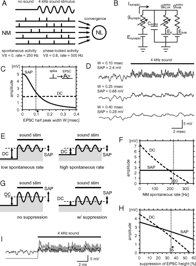
Reproduction of SAP and DC potential in a single-compartment NL neuron model. A, Schematic drawing for the formation of SAP. The convergence of phase-locked synaptic inputs from NM generates both SAP and DC potential in NL. B, Circuit diagram of the model. Note that no somatic Na channels are included. C, Amplitude of SAP and DC potential plotted with respect to half-peak width (W) of unitary inputs from NM. The vertical dotted line indicates the value used in the model (also in F and H, simulated sound frequency = 4 kHz unless otherwise mentioned). D, Examples of voltage traces of the model with three different W values (0.1, 0.25, 0.4 ms). Note that very small value of W (0.1 ms) is needed to reproduce similar amplitudes of SAP observed in vivo experiments. E, Schematic drawings for the effects of spontaneous inputs of NM. Left, Low spontaneous NM spiking rate. Right, High spontaneous NM spiking rate. As the spontaneous rate increases, sound-induced DC shift decreases, while SAP is not affected. F, SAP (solid line) and DC (broken line) potentials plotted with respect to NM spontaneous spike rate. G, Schematic drawings for the effects of sound-induced suppression mechanisms. Left, No suppression in the EPSC amplitude. Right, With suppression in the EPSC amplitude. Sound-induced suppression reduces DC shift more than SAP amplitude. H, SAP (solid line) and DC (broken line) potentials plotted with respect to the sound-induced EPSC suppression ratio. Note that DC decreases more steeply than SAP due to the high spontaneous inputs from NM. I, Comparison of voltage traces with (thin black line) and without (thick gray line) NM spontaneous activity and sound-induced EPSC suppression.

Calculation of binaural synaptic input and SAP.

After calculating two monaural (ipsilateral and contralateral) synaptic conductances (g_ipsi and g_contra) as described above, we obtained binaural synaptic (g_synaptic) inputs by summing the two conductances with different phase delays δ [i.e., g_synaptic^soma(t) = g_ipsi(t) + g_contra(t + T), where T is the time difference between ipsilateral and contralateral inputs and is described as T = (1/f_s) · (δ/360°), where f_s is the signal frequency].

A single compartment passive-soma model of the NL neuron was used to calculate the SAP amplitudes and DC shifts (see Tables 2 and 3 for equations and parameters). The model neuron consisted of a single somatic compartment with leak and low-voltage-activated potassium conductances but without sodium or other active conductances. The amplitudes of SAP and DC shifts were calculated similarly as in the analyses of the experimental data.

Table 2.

Equations of the NL neuron model

Variable	Equation
Compartment	c = soma or node
Membrane potential	$c_{\text{c}}\frac{d}{dt}{V}_{\text{c}}\left(t\right)={/}_{\text{Na}}^{\text{c}}+{/}_{\text{KHVA}}^{\text{c}}+{/}_{\text{KLVA}}^{\text{c}}+{/}_{\text{leak}}^{\text{c}}+{/}_{\text{synaptic}}^{\text{c}}+{/}_{\text{axon}}^{\text{c}}$
Na current	INac = ḡNac · mc hc · (ENa − Vc)
KHVA current	IKHVAc = ḡKHVAc · nc · (EK − Vc)
KLVA current	IKLVAc = ḡKLVAc · dc · (EK − Vc)
Leak current	Ileakc = gleakc · (Eleak − Vc)
Synaptic input	Isynapticc = gsynapticc · (Esynaptic − Vc)
Axonal current	Iaxonsoma = gaxon · (Vnode − Vsoma), Iaxonnode = −Iaxonsoma
Channel variable (x = m, h, n, d)	dxc/dt = φ{αx(Vc) · (1 − xc) − βx(Vc) · xc}
Temperature dependence	φ = Q10(T−23.0)/10(Q10 = 2.5, T = 40°C)
Na channel activation	αm(V) = 3.6exp((V + 34)/7.5), βm(V) = 3.6exp(−(V + 34)/10.0)
Na channel inactivation	αh(V) = 0.6exp(−(V + 57)/18.0), βh(V) = 0.6exp((V + 57)/13.5)
KHVA channel activation	αn(V) = 0.11exp((V + 19)/9.1), βn(V) = 0.103exp(−(V + 19)/20)
KLVA channel activation	αd(V) = 0.2exp((V + 60)/21.8), βd(V) = 0.17exp(−(V + 60)/14)

This table summarizes the equations used in our simulation. In the single-compartment model, I_axon^node = I_axon^soma = 0 and only the somatic compartment was considered.

Table 3.

Parameters used for the NL neuron model

Parameter	Value
Membrane capacitance density	Cm = 1 μF/cm2
Surface of soma	Asoma = 2400 μm2
Surface of node	Anode = 20 μm2
Capacitances	Csoma = CmAsoma = 24 pF, Cnode = CmAnode = 0.2 pF
Reversal potential of Na current	ENa = +35 mV
Reversal potential of K current	EK = −75 mV
Reversal potential of leak current	Eleak = −60 mV
Reversal potential of EPSC	Esynaptic = 0 mV
Sodium conductance densities	GNasoma = 0, GNanode = 7500 mS/cm2
KHVA conductance densities	GKHVAsoma = 0 mS/cm2, GKHVAnode = 2250 mS/cm2
KLVA conductance densities	GKLVAsoma = 8 mS/cm2, GKLVAnode = 40 mS/cm2
Leak conductance densities	Gleaksoma = 2 mS/cm2, Gleaknode = 10 mS/cm2
Maximum Na conductances	ḡNasoma = 0, ḡNanode = 1500 nS
Maximum KHVA conductances	ḡKHVAsoma = 0, ḡKHVAnode = GKHVAnodeAnode = 450 nS
Maximum KLVA conductances	ḡKLVAsoma = GKLVAsomaAsoma = 192 nS, ḡKLVAnode = GKLVAnodeAnode = 8 nS
Leak conductances	gleaksoma = GleaksomaAsoma = 48 nS, gleaknode = GleaknodeAnode = 2 nS
Axonal resistance	ρaxon = 100 Ωcm
Axonal size	Length (between soma and node), Laxon = 60 μm; diameter, Daxon = 3 μm
Axonal conductance	gaxon = (πDaxon2)/(4ρaxonLaxon) = 118 nS

This table summarizes the parameters used in our simulation.

Two-compartment NL neuron model.

The spiking activity of the NL neuron was simulated by a two-compartment passive-soma model as in our previous study (Ashida et al., 2007). The model neuron has two compartments, an unexcitable soma and a spike-initiating node, connected with an axonal resistance (see Tables 2 and 3 for equations and parameters). The membrane potential and ionic currents in each compartment are modeled by Hodgkin–Huxley-type equations (Hodgkin and Huxley, 1952; Koch, 1999). In brief, the large somatic compartment with high-threshold potassium (KLVA) and leak conductances receives synaptic inputs, while the small axonal node compartment with sodium, high-threshold potassium (KHVA), KLVA, and leak conductances generates spikes (see Tables 2 and 3 for equations and parameters). The nodal sodium conductance was determined so that the modulation depth (i.e., difference in spiking rate between best and worst ITDs) would be maximal (see Fig. 8F). The value of the nodal KHVA conductance was chosen so that the membrane potential would repolarize rapidly after spikes. The somatic KLVA and leak conductances were set so that the membrane resistance of the soma at −62 mV would be ∼4.7 MΩ (membrane time constant was ∼0.1 ms), which is similar to the experimental data. The kinetics of the sodium conductance was determined from the previous report on chick NM (Koyano et al., 1996). The kinetics of KLVA and KHVA were taken from the study of chick NM (Rathouz and Trussell, 1998). Numerical integration was performed by using the forward Euler method with a time increment of 0.1 μs.

Figure 8.

Conversion of SAP to spikes in a two-compartment NL model. A, Schematic drawing of two-compartment NL model. B, Circuit diagram of the two-compartment NL model. C, Example of voltage traces of the model with three different simulated phase differences (δ = 0, 90, 180°). D, Spectral profile of the voltage response shown in C. Note that the model reproduces the range of ITD modulation of SAPs and spike rates similar to experimental observations. E, Spike rate modulation with simulated interaural phase differences. The dashed line indicates spontaneous spike rate of the model. F, Spike rate of the model at best (δ = 0°) and worst (δ = 180°) ITDs plotted with respect to the nodal Na conductance. G, Spike rate plotted with respect to artificial sound analog AC inputs at two different nodal Na conductances (bold line, 1.5 μS; thin line, 1.2 μS). The bold broken line (without noise) indicates changes in the spike rate of the model (nodal g_Na = 1.5 μS) to the inputs with only sound analog AC (4 kHz) and DC.

Calculation of AC–rate curves.

AC–rate curves (see Fig. 8F,G) were obtained by injecting sinusoidal input together with background synaptic noise into the model neuron (g_synaptic^soma = g_AC · sin(2πf_st) + g_noise, where f_s is the signal frequency). SAP amplitude and spiking rate were calculated with varying g_AC. Synaptic noise g_noise was constructed from the same model of NM activity described above assuming VS = 0. SAP–firing rate curves without noise was obtained by varying AC and maintaining DC inputs constant (g_synaptic^soma = g_AC · sin(2πf_st) + g_DC). g_DC was fixed to the averaged input level of the simulated noisy synaptic input g_noise.

Results

Intracellular responses of NL neurons

We obtained in vivo intracellular data from 35 NL cells in 9 of 16 owls. In the other seven owls, only extracellular unit recordings were obtained. Since we recorded from the caudal third of NL, where cell density is higher than in other regions (Carr and Boudreau, 1993a), best frequencies (frequency of sounds where cells respond most) were centered around 3 kHz (ranging 0.8–5.6 kHz; 3.2 ± 1.0 kHz; n = 35).

NL neurons produced somatic spikes of unusually small amplitude (9 ± 3 mV; n = 35), and membrane potentials resembling the waveform of the tonal stimulus even during the falling phase of spikes (Fig. 1Bd). We called these potentials sound analog potentials or SAPs. Indicative of an intracellular origin for the oscillatory potentials, spectral analysis of the voltage traces showed a peak at the stimulus frequency, whose power suddenly increased after penetration (2.2 times larger on average; 2.2 ± 1.2; n = 30; Fig. 1Bc).

Response to ITD

We recorded ITD-dependent changes in membrane potential and spike rate with tonal stimuli in 24 neurons. The ITD that elicited the largest number of spikes always elicited the largest SAPs (Fig. 2A–E). The firing rate of NL neurons varied linearly with the amplitude of SAPs (r = 0.91; p < 0.0001; Fig. 2G). Recordings from low BF cells (<1.5 kHz; Fig. 3) were qualitatively similar to those for high BF cells except that spikes occurred in almost every tonal cycle during the first half of sound stimuli with favorable ITDs (Fig. 3Ba, 0.9 kHz). For the least favorable ITD (the ITD with which cells generate the least spikes), SAPs were hardly visible in the spectrogram of voltage traces (Fig. 2Cc). Sound-evoked DC shifts (Fig. 2Ac and Materials and Methods for definition) did not show a similar clear ITD dependency (Fig. 2F,H; r = −0.13; p > 0.1).

Figure 3.

ITD-dependent changes in membrane potential in low-frequency NL neuron. A, ITD was varied for a tone burst stimulus (0.9 kHz; 60 ms duration; bar above traces). a, Most favorable ITD (−270 μs). b, An intermediate ITD (0 μs). c, Least favorable ITD (270 μs). The broken line shows the level of −75 mV. B, Expanded traces from A (Aa, short bar below trace). C, Spectral analysis of membrane potentials shown in A. Findings are in principle the same as high-frequency NL cells (Fig. 2), although small spectral powers of second and third harmonics of the stimulus tones are visible especially at the onset of sound stimuli with favorable ITD. D, Spike rates plotted against ITD. E, SAP amplitude plotted against ITD. F, DC shift evoked by sound plotted against ITD. The horizontal axis is shared with D and E. G, Spike rate plotted against SAP amplitude. H, Spike rate plotted with respect to DC shift.

In all the cells recorded, the spike rate of NL neurons was highly correlated with the amplitude of SAPs (r = 0.88 ± 0.07; n = 24), whereas a significant correlation was rarely observed between sound-evoked DC shifts and spike rate (r = 0.09 ± 0.34; n = 24; Fig. 4A). Both NL spike rates and the amplitude of SAPs exhibited strikingly similar relationships to ITD (Fig. 2D,E). When rate–ITD and SAP–ITD curves were fitted with a sinusoidal function matching the stimulus frequency, the phase difference between the two ITD curves was small (7.5 ± 6.3°; n = 24; Fig. 4B). However, DC shifts as a function of ITD failed to show a clear relationship with rate–ITD curves. When rate–ITD and DC-shift ITD curves were fitted with sinusoidal functions matching the stimulus frequency, the phase difference between the two ITD curves was large (84.7 ± 58.4°; n = 24).

Figure 4.

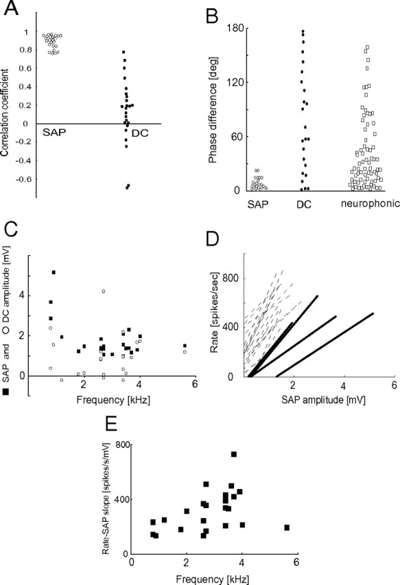
Sound analog and DC potentials in NL neurons. A, Correlation coefficient measured for plots of SAP amplitude versus spike rate (SAP, as in Figs. 2G, 3G), and sound-evoked DC shift versus spike rate (DC, as in Figs. 2H, 3H), for 24 cells. B, Measured phase differences between the recorded SAP amplitude and spike rate (SAP; e.g., Fig. 2, compare D, E) when fitted with a sine curve with the same frequency of the stimulus tone. Phase differences between the sound-evoked DC potential and the spike rate ITD curve (DC; e.g., Fig. 2, compare D, F), and phase differences between the neurophonic amplitude curve and the extracellular spike rate ITD curve (neurophonic). C, Maximum SAPs (SAP, filled squares) and averaged sound-evoked DC shifts (DC, open circles) plotted with respect to the BF of the cell. D, SAP versus firing rate curves (rate–SAP curve) for all 24 neurons. Each line shows a linear regression line of rate–SAP curve for each cell. The four solid lines are from the lowest frequency neurons (BF < 1.5 kHz). The dotted lines are from higher frequency neurons (BF > 1.5 kHz). E, Slope of rate–SAP curve plotted with respect to the BF of the cell.

A large extracellular field potential, called the neurophonic, characterizes extracellular recordings in NLs (Sullivan and Konishi, 1986; Kuokkanen et al., 2010). Interestingly, during extracellular recording of NL neurons, the phase difference between rate–ITD curves and neurophonic amplitude–ITD curves recorded at the same time was sometimes large (41.3 ± 40.3°; n = 75). This phase mismatch may be due to recording from NL axons at some distance from their cell bodies. Since the axons of NL cells run along the gradient of ITDs in the nucleus (Sullivan and Konishi, 1986; Carr and Boudreau, 1993a), the ITD selectivity of NL axons may differ from that of the local field potential. However, the negligible phase difference between the SAP and the spike rate suggests that intracellular recordings were obtained from the cell bodies of NL neurons.

Difference between high and low best frequency cells

The amplitude of SAPs decreased with increasing BF (ρ = −0.45; n = 24; p = 0.035; Spearman's rank correlation; Fig. 4C). The maximum amplitude was ∼2 mV (1.74 ± 0.93 mV; n = 24). The sound-evoked DC shift (0.87 ± 1.1 mV) did not show significant correlation with BF (ρ = 0.16; n = 24; p = 0.44; Spearman's rank correlation). The shape of curves of firing rate as a function of SAP amplitude differed between low BF (<1.5 kHz; n = 4; Fig. 4D, solid lines) and high BF cells (>1.5 kHz; n = 20; Fig. 4D, broken lines). Low BF cells did not show large increases in firing rate for small changes in SAP (e.g., <1 mV). In contrast, high BF cells were surprisingly sensitive to small changes in SAPs. The slope of firing rate versus SAP amplitude curves showed significant correlation to the BFs of the cells (ρ = 0.48; n = 24; p = 0.023; Spearman's rank order correlation; Fig. 4E).

The spike shape of low BF NL cells differed from that of high BF cells (Fig. 5A). The spike height was not correlated with the BF of the cells (r = 0.03; n = 35; p = 0.87; Fig. 5B); however, the half-width of spikes was significantly correlated (r = 0.34; n = 35; p = 0.045; Fig. 5C). High best frequency cells showed broader spikes than low best frequency cells.

To estimate the excitability of the neuron, we measured the increase in firing rate evoked by small positive currents (0.3 nA, 15–20 ms) and plotted against their BFs (Fig. 6B). The firing rate increase was significantly correlated with the BF of the cell (r = 0.41; p = 0.025; n = 30). None of the low BF cells (<1.5 kHz; n = 4) showed clear increase in spike rate with this amount of current; however, most high BF cells (>1.5 kHz; n = 26) showed a clear increase. Thus, high BF cells showed higher excitability to injected current than low BF cells.

Spontaneous voltage traces of low BF cells showed large fluctuations (Figs. 3A, 5Ac, 6Ac,d). We measured the SD of membrane potentials when neither sound nor current pulses were applied and removing periods of spontaneous spikes. The SD of membrane voltages showed clear negative correlation with the BF of a cell (Fig. 6C; r = −0.61; p < 0.0001; n = 35). Thus, putative synaptic noise in low BF cells is larger than that in high BF cells.

Reproduction of experimental findings in an NL model

Our recordings from owl's NL cells in vivo have revealed characteristic sound-induced responses, including SAPs, small spikes, and linear conversion from SAPs to spikes. To investigate their underlying biophysical mechanisms, we modeled NL neurons.

First, we used a single-compartment model representing the NL cell body to reproduce SAP and DC potentials by synaptic integration (Fig. 7A,B). We have already shown that spike generation at the small first node does not significantly affect the formation of SAP and DC potential in the somata (Ashida et al., 2007). Convergence of phase-locked NM inputs can give rise to SAP and DC potential in NL (Fig. 7A). The “volley theory” gives an underlying principle to the emergence of a copy of the sound waveform in the membrane potential of NL cells. Thus, high-frequency sounds of >1.5 kHz can be reproduced by many phase-locked inputs coming in volleys (Wever and Bray, 1930).

In our simulation, we set the spontaneous firing rate of NM at 220 spikes/s (Köppl, 1997a), and the evoked firing rate at 500 spikes/s (Peña et al., 1996). The stimulus sound frequency was arbitrarily set to 4 kHz, because the experimental data around this frequency is abundant and because, at this relatively high frequency, the task of generating SAPs becomes more demanding (Ashida et al., 2007). The vector strength (a parameter indicating the degree of phase-locking) of NM axons was set to 0.6 (Köppl, 1997b), and the number of converging NM axons from either side to one NL was fixed to 150 (Carr and Boudreau, 1993a). Detailed descriptions of the parameters used in the simulation are listed in Table 1. As a starting point, we considered only binaural inputs with perfect coincidence (i.e., there is no phase delays between ipsilateral and contralateral inputs). Note that the model neuron receives 300 (150 fibers from each side) × 500 (spikes/s)/4000 (Hz) = 37.5 phase-locked inputs (on average) for each cycle of the stimulus. Since our experimental observations revealed a few millivolts of SAPs around 4 kHz at favorable ITD and slightly smaller DC depolarization with binaural tonal stimuli, we looked for parameter sets in which the model showed similar amplitudes of SAP and DC potential. When the DC amplitude was kept constant (1.8 mV in this case), the model required very fast excitatory inputs to create SAPs of a few millivolts at 4 kHz (Fig. 7C,D). If the half-peak width (W) of an unitary EPSC coming from a NM axon is set to 0.25 ms, which is close to the reported experimental data recorded in young chicken NL cells with high BFs (Kuba et al., 2005; Slee et al., 2010), SAPs did not exceed 1 mV on average. An even shorter W of ∼0.1 ms was required to create SAPs of a few millivolts. We therefore used a value of 0.1 for W in further simulations.

The small DC potential shift (1.8 mV in this case; Fig. 7C,D) was determined by several parameters of the model. One of the most influential parameter was the spontaneous firing rate of NM axons, which is high in owls (Köppl, 1997a). Since the DC shift was defined as the difference between the membrane potentials before and during sound stimulation (Fig. 2A,B), an increase in the spontaneous input can directly reduce the amplitude of the DC shift (Fig. 7E,F). We also incorporated a sound-induced suppression mechanism of synaptic inputs (Fig. 7G,H; potential candidates are discussed later). Suppression in the synaptic input decreased both the DC shift and SAP amplitude. The DC shift, however, is more likely to decrease because of the spontaneous inputs (Fig. 7G,H). With the spontaneous NM spike rate (220 Hz) roughly one-half of the sound-induced one (500 Hz), and sound-induced suppression (to 65% when sound is on) of synaptic inputs, the DC shift was reduced from 9.8 mV (neither spontaneous NM activity nor sound-induced suppression were incorporated) to 1.8 mV (Fig. 7I).

We added a spike generator (i.e., Na channels in the first node of Ranvier) to the model neuron to model linear conversion of SAPs to spikes [Fig. 8A,B; described in detail by Ashida et al. (2007)]. Keeping the simulated binaural inputs the same as in Figure 7, the model showed ITD-dependent firing rate modulation as the nodal Na channel density increased (Fig. 8C–F). When the nodal Na channel density was 1.5 μS, the model showed 470 spikes/s for the favorable ITD (δ = 0°; SAP = 2.4 mV), and 180 spikes/s for the unfavorable ITD (δ = 180°; SAP = 0 mV) (Fig. 8C,E,F).

The firing rate–SAP curve showed a smooth monotonic increase (Fig. 8G, “in vivo range”). We further tested the AC sensitivity of the model by artificially increasing the amplitude of sound analog signals (AC, 4 kHz) without altering other frequency components (Fig. 8G, with noise; see Material and Methods). A model with smaller nodal Na channel density (nodal g_Na = 1.2 μS; Fig. 8G, thin line) could change spike rate when AC amplitude exceeded 3 mV, which was larger than the in vivo range for high BF cells. These results indicate that the required Na conductance is less for sensing large AC signals (i.e., large SAP). This result may explain the lower excitability of low BF cells in vivo, which show large SAPs (Figs. 4C, 6B).

Synaptic convergence from hundreds of NM neurons to one NL neuron creates not only SAPs and DC potentials but also other frequency components, which appear as “noise” (Fig. 7D). When these additional components were removed from the inputs (Fig. 8G, “without noise”), the model with 1.5 μS nodal Na conductance lost responsiveness to AC changes <5 mV, indicating that the synaptic noise may lower the threshold for sensing the SAP (AC) by linearizing the rate–SAP curve. This result indicates that synaptic noise is one of the underlying mechanisms of the linear conversion (Figs. 2G, 3G, 4D) from SAP to firing rate in NL.

Discussion

In vivo intracellular recording using coaxial electrode

We used coaxial glass electrodes to obtain intracellular recording in NL. This configuration permitted repeated intracellular recordings from a deep brain area (deeper than 5 mm from the brain surface) in the same animal. With this technique, it was unnecessary to perform more invasive, terminal, procedures such as removing the cerebellum to access NL.

Signal coding ITD

We found that the signal that determines spike rate is not a DC potential, but a sound analog, AC potential in NL cells in vivo. To our knowledge, there are no other examples of in vivo recordings of neurons that encode AC signals in the kilohertz range, far faster and shorter than the duration of a spike, to trigger spikes. Probably cochlear hair cells are similar, because they also show sound analog receptor potentials in the kilohertz range with tonal stimuli, although hair cells do not generate spikes (Russell and Sellick, 1978).

In general, we rarely saw large second and third harmonic components of SAPs in the spectrogram of membrane responses except during the period of onset bursting that we occasionally observed in response to favorable ITDs (Figs. 2C, 3C). In some of the low-frequency cells, we sometimes saw second harmonic components with unfavorable ITDs, although their amplitude was not large (Fig. 3Cc). It is possible that the reason we did not see substantial second harmonics of SAPs in the membrane potential may be due to the fact that high-frequency components of the response, such as second and third harmonics, are attenuated by the low-pass filter properties of the soma (Ashida et al., 2007). If neurons were to tuned to show larger second harmonic components, this could disturb ITD computation, because second harmonic components at unfavorable ITDs can be as large as the responses at favorable ITDs (Reyes et al., 1996; Slee et al., 2010).

Analysis of SAP

In measuring SAP amplitude, we removed spikes from analysis (see Materials and Methods; Fig. 1). As shown in Figures 1Bd, 2Ba, and 3, Ba and Bb, the SAP amplitude showed some fluctuation. The probability of firing will be affected by the amplitude of the voltage oscillations during each cycle of the SAP. Thus, the voltage fluctuations in cycles where spikes are not generated may be smaller than those with spikes, which are removed from analysis. Therefore, the actual SAP amplitudes generated in NL cells in vivo might be larger than those shown in Figures 2E, 3E, and 4C.

Comparison with other biophysical studies of auditory coincidence detectors

The owl's NL neurons produced only small somatic spikes (9 ± 3 mV; n = 35) in vivo. This phenomenon has been observed in in vitro studies of NL cells in posthatch chicks (Kuba et al., 2006), neurons of the medial superior olivary nucleus (MSO) of the gerbil (Scott et al., 2005), and octopus cells of the anteroventral cochlear nucleus (Golding et al., 1999), but was not previously confirmed in vivo.

The initial segment of NL axon is myelinated (Carr and Boudreau, 1993b), suggesting that action potentials may be initiated at the first node of Ranvier, located 60 μm away from the soma. SAPs were observed even during the falling phase of spikes (Figs. 1Bd, 2Ba). This indicates that conductance for spike generation does not override synaptic conductances (Häusser et al., 2001). This is also consistent with a remote spike initiation site. Remote spike initiation may allow for a lower spike threshold at the spike initiation site, by filtering DC potentials that could inactivate Na channels (Kuba et al., 2006). This configuration could also amplify high-frequency signals at the spike initiation site (Ashida et al., 2007), decreasing backpropagation (Golding et al., 1999; Scott et al., 2005, 2007), and reducing the metabolic cost of high-frequency firing (Ashida et al., 2007).

The input resistance of NL cells was low (10.4 ± 8.2; n = 33). A low input resistance contributes to the short membrane time constant, which is thought to be necessary for ITD computation (Gerstner et al., 1996). Similar low input resistance has also been reported in other auditory coincidence detectors such as the NL neurons of posthatch chicks (Kuba et al., 2005, 2006) and the mammalian MSO (Scott et al., 2005).

Small positive-current injections (e.g., 0.3 nA) generated repeated firing in NL cells with high BFs (Figs. 1Bb, 6Aa,b). Phasic firing with current injection has long been regarded as one of the important features of time-coding auditory neurons (Oertel, 1983; Reyes et al., 1996). The major difference between our in vivo observation and the in vitro observations are the frequency range that NL cells cover, and the existence of spontaneous inputs. No matter how many low-voltage activated potassium channels (KLVA), long been supposed to be a key for phasic firing (Manis and Marx, 1991; Svirskis et al., 2004), were incorporated, the model cells generated multiple spikes to current injection as nodal Na channels were increased (Ashida et al., 2007). Also, even in models with phasic firing, adding noise or high-frequency components sometimes induces multiple spikes (Higgs et al., 2006).

To reproduce a few millivolts of SAP at 4 kHz and slightly less DC potentials in our model, it was necessary to incorporate extraordinarily fast EPSCs and suppressing mechanisms, which is “on” during sound stimulation (Fig. 7; see below). The duration of unitary EPSC hypothesized (W = 0.1 ms) is less than one-half of those reported previously in chicken NL (Kuba et al., 2005; Slee et al., 2010). Since the frequency range that the owl's NL neurons respond is much larger than that of the chicken NL [owls, up to 8 kHz (Carr and Konishi, 1990; Köppl and Carr, 2008); chickens, up to 3.8 kHz (Rubel and Parks, 1975)], owl NL EPSCs might be specially tuned to higher frequency signals. In vitro measurement of actual EPSCs in owl's NL will be necessary to test the prediction of our model. GABAergic inhibition (Carr et al., 1989; Lachica et al., 1994; Funabiki et al., 1998; Yang et al., 1999; Burger et al., 2005) and synaptic depression (Kuba et al., 2002; Cook et al., 2003; Slee et al., 2010) are candidates for sound-induced suppression mechanisms of synaptic inputs in NL. In our experimental observation, sound-evoked DC shifts did not change with ITD (Figs. 2F, 3F), although NL spike rates changed with the level of steady depolarization (Fig. 1C). This suggests that, although sound-evoked DC shifts do not play a major role in ITD coding, they could disturb ITD computation, if they are large and fluctuating. Furthermore, sound-evoked DC shifts did not increase with increasing BF (Fig. 4C), although this has been expected as a consequence of temporal summation (Kuba et al., 2006). The modeling results (Fig. 7E–I) suggest that the combination of the high spontaneous rate of NM neurons and the sound-induced suppression mechanisms of EPSC can account for the DC suppression in vivo.

Difference between high and low best frequency NL cells

Although spike height did not correlate with the BF of the cell, the spike width did (Fig. 5). Spike initiation sites are reported to show a change with the BF of the cell in the chicken NL (Kuba et al., 2006). The shapes of spontaneous spikes in the owl's high-frequency NL cells (Fig. 5A) resembled those of antidromically evoked spikes in the chicken NL (Kuba et al., 2006). Thus, the distance between the cell body and the spike initiation site might differ between high and low BF NL cells in barn owls.

Spontaneous voltage traces of high BF cells are less noisy than those of low BF cells (Fig. 6). Although synaptic noise can lower the threshold for detecting small AC (SAP) signals (Fig. 8G), too much noise would interfere with the computation because of the higher excitability of high BF NL cells (Fig. 6B). Thus, not only the excitability but also the strategy of optimization of synaptic noise may differ between cells with different BF.

The reproduction of sound waveforms in membrane potential of NL neurons is consistent with several biophysical parameters. The large somatic capacitance acts as a low-pass filter, whereas several types of outward currents act as high-pass filters (Ashida et al., 2007; Slee et al., 2010). Remote spiking at a small compartment, such as the first node of Ranvier, will also act as a high-frequency amplifier (Ashida et al., 2007). The width of the unitary excitatory input and the number of converging inputs will also affect the spectral profile of the synaptic potential. In the chicken NL, dendritic length (Smith and Rubel, 1979), width of EPSCs (Kuba et al., 2005; Slee et al., 2010), intrinsic membrane properties (Kuba et al., 2005; Slee et al., 2010), and spike initiation sites (Kuba et al., 2006) show gradual changes along the frequency axis. Reviewing these facts with regard to the generation and computation of SAPs will become an important issue for further observation.

References

- Agmon-Snir H, Carr CE, Rinzel J. The role of dendrites in auditory coincidence detection. Nature. 1998;393:268–272. doi: 10.1038/30505. [DOI] [PubMed] [Google Scholar]
- Ashida G, Abe K, Funabiki K, Konishi M. Passive soma facilitates submillisecond coincidence detection in the owl's auditory system. J Neurophysiol. 2007;97:2267–2282. doi: 10.1152/jn.00399.2006. [DOI] [PubMed] [Google Scholar]
- Burger RM, Cramer KS, Pfeiffer JD, Rubel EW. Avian superior olivary nucleus provides divergent inhibitory input to parallel auditory pathways. J Comp Neurol. 2005;481:6–18. doi: 10.1002/cne.20334. [DOI] [PubMed] [Google Scholar]
- Carr CE, Boudreau RE. Organization of the nucleus magnocellularis and the nucleus laminaris in the barn owl: encoding and measuring interaural time differences. J Comp Neurol. 1993a;334:337–355. doi: 10.1002/cne.903340302. [DOI] [PubMed] [Google Scholar]
- Carr CE, Boudreau RE. An axon with a myelinated initial segment in the bird auditory system. Brain Res. 1993b;628:330–334. doi: 10.1016/0006-8993(93)90975-s. [DOI] [PubMed] [Google Scholar]
- Carr CE, Konishi M. A circuit for detection of interaural time differences in the brainstem of the barn owl. J Neurosci. 1990;10:3227–3246. doi: 10.1523/JNEUROSCI.10-10-03227.1990. [DOI] [PMC free article] [PubMed] [Google Scholar]
- Carr CE, Fujita I, Konishi M. Distribution of GABAergic neurons and terminals in the auditory system of the barn owl. J Comp Neurol. 1989;286:190–207. doi: 10.1002/cne.902860205. [DOI] [PubMed] [Google Scholar]
- Cook DL, Schwindt PC, Grande LA, Spain WJ. Synaptic depression in the localization of sound. Nature. 2003;421:66–70. doi: 10.1038/nature01248. [DOI] [PubMed] [Google Scholar]
- Fischer BJ, Christianson GB, Peña JL. Cross-correlation in the auditory coincidence detectors of owls. J Neurosci. 2008;28:8107–8115. doi: 10.1523/JNEUROSCI.1969-08.2008. [DOI] [PMC free article] [PubMed] [Google Scholar]
- Funabiki K, Koyano K, Ohmori H. The role of GABAergic inputs for coincidence detection in the neurones of nucleus laminaris of the chick. J Physiol. 1998;508:851–869. doi: 10.1111/j.1469-7793.1998.851bp.x. [DOI] [PMC free article] [PubMed] [Google Scholar]
- Gerstner W, Kempter R, van Hemmen JL, Wagner H. A neural learning role for sub-millisecond temporal coding. Nature. 1996;383:76–81. doi: 10.1038/383076a0. [DOI] [PubMed] [Google Scholar]
- Golding NL, Ferragamo MJ, Oertel D. Role of intrinsic conductances underlying responses to transients in octopus cells of the cochlear nucleus. J Neurosci. 1999;19:2897–2905. doi: 10.1523/JNEUROSCI.19-08-02897.1999. [DOI] [PMC free article] [PubMed] [Google Scholar]
- Grau-Serrat V, Carr CE, Simon JZ. Modeling coincidence detection in nucleus laminaris. Biol Cybern. 2003;89:388–396. doi: 10.1007/s00422-003-0444-4. [DOI] [PMC free article] [PubMed] [Google Scholar]
- Grothe B, Pecka M, McAlpine D. Mechanisms of sound localization in mammals. Physiol Rev. 2010;90:983–1012. doi: 10.1152/physrev.00026.2009. [DOI] [PubMed] [Google Scholar]
- Häusser M, Major G, Stuart GJ. Differential shunting of EPSPs by action potentials. Science. 2001;291:138–141. doi: 10.1126/science.291.5501.138. [DOI] [PubMed] [Google Scholar]
- Higgs MH, Slee SJ, Spain WJ. Diversity of gain modulation by noise in neocortical neurons. J Neurosci. 2006;26:8787–8799. doi: 10.1523/JNEUROSCI.1792-06.2006. [DOI] [PMC free article] [PubMed] [Google Scholar]
- Hodgkin AL, Huxley AF. A quantitative description of membrane currents and its application to conduction and excitation in nerve. J Physiol. 1952;117:500–544. doi: 10.1113/jphysiol.1952.sp004764. [DOI] [PMC free article] [PubMed] [Google Scholar]
- Jeffress LA. A place theory of sound localization. J Comp Physiol Psychol. 1948;41:35–39. doi: 10.1037/h0061495. [DOI] [PubMed] [Google Scholar]
- Knudsen EI, Blasdel GG, Konishi M. Sound localization by the barn owl (Tyto alba) measured with the search coil technique. J Comp Physiol A Neuroethol Sens Neural Behav Physiol. 1979;133:1–11. [Google Scholar]
- Koch C. Biophysics of computation. New York: Oxford UP; 1999. [Google Scholar]
- Konishi M. Listening with two ears. Sci Am. 1993;268:66–73. doi: 10.1038/scientificamerican0493-66. [DOI] [PubMed] [Google Scholar]
- Köppl C. Frequency tuning and spontaneous activity in the auditory nerve and cochlear nucleus magnocellularis of the barn owl Tyto alba. J Neurophysiol. 1997a;77:364–377. doi: 10.1152/jn.1997.77.1.364. [DOI] [PubMed] [Google Scholar]
- Köppl C. Phase locking to high frequencies in the auditory nerve and cochlear nucleus magnocellularis of the barn owl, Tyto alba. J Neurosci. 1997b;17:3312–3321. doi: 10.1523/JNEUROSCI.17-09-03312.1997. [DOI] [PMC free article] [PubMed] [Google Scholar]
- Köppl C, Carr CE. Maps of interaural time difference in the chicken's brainstem nucleus laminaris. Biol Cybern. 2008;98:541–559. doi: 10.1007/s00422-008-0220-6. [DOI] [PMC free article] [PubMed] [Google Scholar]
- Koyano K, Funabiki K, Ohmori H. Voltage-gated ionic currents and their roles in timing coding in auditory neurons of the nucleus magnocellularis of the chick. Neurosci Res. 1996;26:29–45. doi: 10.1016/0168-0102(96)01071-1. [DOI] [PubMed] [Google Scholar]
- Kuba H, Koyano K, Ohmori H. Synaptic depression improves coincidence detection in the nucleus laminaris in brainstem slices of the chick embryo. Eur J Neurosci. 2002;15:984–990. doi: 10.1046/j.1460-9568.2002.01933.x. [DOI] [PubMed] [Google Scholar]
- Kuba H, Yamada R, Fukui I, Ohmori H. Tonotopic specialization of auditory coincidence detection in nucleus laminaris of the chick. J Neurosci. 2005;25:1924–1934. doi: 10.1523/JNEUROSCI.4428-04.2005. [DOI] [PMC free article] [PubMed] [Google Scholar]
- Kuba H, Ishii TM, Ohmori H. Axonal site of spike initiation enhances auditory coincidence detection. Nature. 2006;444:1069–1072. doi: 10.1038/nature05347. [DOI] [PubMed] [Google Scholar]
- Kuokkanen PT, Wagner H, Ashida G, Carr CE, Kempter R. On the origin of the extracellular field potential in the nucleus laminaris of the barn owl (Tyto alba) J Neurophysiol. 2010;104:2274–2290. doi: 10.1152/jn.00395.2010. [DOI] [PMC free article] [PubMed] [Google Scholar]
- Lachica EA, Rübsamen R, Rubel EW. GABAergic terminals in nucleus magnocellularis and laminaris originate from the superior olivary nucleus. J Comp Neurol. 1994;348:403–418. doi: 10.1002/cne.903480307. [DOI] [PubMed] [Google Scholar]
- Manis PB, Marx SO. Outward currents in isolated ventral cochlear nucleus neurons. J Neurosci. 1991;11:2865–2880. doi: 10.1523/JNEUROSCI.11-09-02865.1991. [DOI] [PMC free article] [PubMed] [Google Scholar]
- Oertel D. Synaptic responses and electrical properties of cells in brain slices of the mouse anteroventral cochlear nucleus. J Neurosci. 1983;3:2043–2053. doi: 10.1523/JNEUROSCI.03-10-02043.1983. [DOI] [PMC free article] [PubMed] [Google Scholar]
- Peña JL, Viete S, Albeck Y, Konishi M. Tolerance to sound intensity of binaural coincidence detection in the nucleus laminaris of the owl. J Neurosci. 1996;16:7046–7054. doi: 10.1523/JNEUROSCI.16-21-07046.1996. [DOI] [PMC free article] [PubMed] [Google Scholar]
- Peña JL, Viete S, Funabiki K, Saberi K, Konishi M. Cochlear and neural delays for coincidence detection in owls. J Neurosci. 2001;21:9455–9459. doi: 10.1523/JNEUROSCI.21-23-09455.2001. [DOI] [PMC free article] [PubMed] [Google Scholar]
- Rathouz M, Trussell L. Characterization of outward currents in neurons of the avian nucleus magnocellularis. J Neurophysiol. 1998;80:2824–2835. doi: 10.1152/jn.1998.80.6.2824. [DOI] [PubMed] [Google Scholar]
- Reyes AD, Rubel EW, Spain WJ. In vitro analysis of optimal stimuli for phase-locking and time-delayed modulation of firing in avian nucleus laminaris neurons. J Neurosci. 1996;16:993–1007. doi: 10.1523/JNEUROSCI.16-03-00993.1996. [DOI] [PMC free article] [PubMed] [Google Scholar]
- Rubel EW, Parks TN. Organization and development of brain stem auditory nuclei of the chicken: tonotopic organization of N. magnocellularis and N. laminaris. J Comp Neurol. 1975;164:411–433. doi: 10.1002/cne.901640403. [DOI] [PubMed] [Google Scholar]
- Russell IJ, Sellick PM. Intracellular studies of hair cells in the mammalian cochlea. J Physiol. 1978;284:261–290. doi: 10.1113/jphysiol.1978.sp012540. [DOI] [PMC free article] [PubMed] [Google Scholar]
- Sachs F, McGarrigle R. An almost completely shielded microelectrode. J Neurosci Methods. 1980;3:151–157. doi: 10.1016/0165-0270(80)90022-9. [DOI] [PubMed] [Google Scholar]
- Schwartz TL, House CR. A small-tipped microelectrode designed to minimize capacitive artifacts during the passage of current through the bath. Rev Sci Instrum. 1970;41:515–517. doi: 10.1063/1.1684564. [DOI] [PubMed] [Google Scholar]
- Scott LL, Mathews PJ, Golding NL. Posthearing developmental refinement of temporal processing in principal neurons of the medial superior olive. J Neurosci. 2005;25:7887–7895. doi: 10.1523/JNEUROSCI.1016-05.2005. [DOI] [PMC free article] [PubMed] [Google Scholar]
- Scott LL, Hage TA, Golding NL. Weak action potential backpropagation is associated with high-frequency axonal firing capability in principal neurons of the gerbil medial superior olive. J Physiol. 2007;583:647–661. doi: 10.1113/jphysiol.2007.136366. [DOI] [PMC free article] [PubMed] [Google Scholar]
- Slee SJ, Higgs MH, Fairhall AL, Spain WJ. Tonotopic tuning in a sound localization circuit. J Neurophysiol. 2010;103:2857–2875. doi: 10.1152/jn.00678.2009. [DOI] [PMC free article] [PubMed] [Google Scholar]
- Smith DJ, Rubel EW. Organization and development of brain stem auditory nuclei of the chicken: dendritic gradients in nucleus laminaris. J Comp Neurol. 1979;186:213–239. doi: 10.1002/cne.901860207. [DOI] [PubMed] [Google Scholar]
- Sullivan WE, Konishi M. Neural map of interaural phase difference in the owl's brainstem. Proc Natl Acad Sci U S A. 1986;83:8400–8404. doi: 10.1073/pnas.83.21.8400. [DOI] [PMC free article] [PubMed] [Google Scholar]
- Svirskis G, Kotak V, Sanes DH, Rinzel J. Sodium along with low-threshold potassium currents enhance coincidence detection of subthreshold noisy signals in MSO neurons. J Neurophysiol. 2004;91:2465–2473. doi: 10.1152/jn.00717.2003. [DOI] [PMC free article] [PubMed] [Google Scholar]
- Trussell LO. Synaptic mechanisms for coding timing in auditory neurons. Annu Rev Physiol. 1999;61:477–496. doi: 10.1146/annurev.physiol.61.1.477. [DOI] [PubMed] [Google Scholar]
- Wever EG, Bray CW. Action currents in the auditory nerve in response to acoustical stimulation. Proc Natl Acad Sci U S A. 1930;16:344–350. doi: 10.1073/pnas.16.5.344. [DOI] [PMC free article] [PubMed] [Google Scholar]
- Yang L, Monsivais P, Rubel EW. The superior olivary nucleus and its influence on nucleus laminaris: a source of inhibitory feedback for coincidence detection in the avian auditory brainstem. J Neurosci. 1999;19:2313–2325. doi: 10.1523/JNEUROSCI.19-06-02313.1999. [DOI] [PMC free article] [PubMed] [Google Scholar]