Unravelling the Intrinsic Functional Organization of the Human Lateral Frontal Cortex: A Parcellation Scheme Based on Resting State fMRI

Abstract

Human and nonhuman primates exhibit flexible behavior. Functional, anatomical, and lesion studies indicate that the lateral frontal cortex (LFC) plays a pivotal role in such behavior. LFC consists of distinct subregions exhibiting distinct connectivity patterns that possibly relate to functional specializations. Inference about the border of each subregion in the human brain is performed with the aid of macroscopic landmarks and/or cytoarchitectonic parcellations extrapolated in a stereotaxic system. However, the high interindividual variability, the limited availability of cytoarchitectonic probabilistic maps, and the absence of robust functional localizers render the in vivo delineation and examination of the LFC subregions challenging. In this study, we use resting state fMRI for the in vivo parcellation of the human LFC on a subjectwise and data-driven manner. This approach succeeds in uncovering neuroanatomically realistic subregions, with potential anatomical substrates including BA 46, 44, 45, 9 and related (sub)divisions. Ventral LFC subregions exhibit different functional connectivity (FC), which can account for different contributions in the language domain, while more dorsal adjacent subregions mark a transition to visuospatial/sensorimotor networks. Dorsal LFC subregions participate in known large-scale networks obeying an external/internal information processing dichotomy. Furthermore, we traced “families” of LFC subregions organized along the dorsal–ventral and anterior–posterior axis with distinct functional networks also encompassing specialized cingulate divisions. Similarities with the connectivity of macaque candidate homologs were observed, such as the premotor affiliation of presumed BA 46. The current findings partially support dominant LFC models.

Introduction

Human and nonhuman primates are characterized by flexible behavior. Processes such as learning, integration of information, and rule following are essential for the successful interaction with the environment and the accomplishment of everyday tasks. The frontal lobe has been identified as the brain structure that plays a pivotal role in these “higher order” processes (Goldman-Rakic, 1996; Miller and Cohen, 2001). The lateral frontal cortex (LFC) is especially implicated in diverse aspects of task execution (Koechlin et al., 2003; Brass et al., 2005; Stiers et al., 2010).

The LFC, like the rest of the cortex, is far from homogeneous. Several LFC cytoarchitectonic parcellation schemes have appeared for the human brain, with variations in the number and extent of LFC divisions (Brodmann, 1909; Sarkissov et al., 1955; Petrides and Pandya, 1994) (Fig. 1). Moreover, tracing studies in the monkey and rodent frontal cortex have demonstrated that regions differentiated through their cytoarchitecture also exhibit different connectivity patterns (Uylings et al., 2003; Yeterian et al., 2011). This “connectivity fingerprint” of each region seems to reflect a functional specialization, in line with evidence from lesion studies (Passingham et al., 2002; Petrides, 2005). The proper function and extensive repertoire of the LFC appears to rely on the interaction of these specialized regions (Miller, 2000; Wilson et al., 2010). Consequently, their delineation and the further characterization of their connectivity properties are crucial for better understanding of the LFC.

Figure 1.

A–C, Cytoarchitectonic parcellations of the human lateral frontal cortex based on Brodmann (1909) (A), Sarkissov et al. (1955) (B), and Petrides and Pandya (1994) (C). Note the variability in the shape and extent of the same region in each parcellation scheme (e.g., region 46 in A and B). Note also the differences in the number of divisions (e.g., region 9 appears homogeneous in B, whereas it is further subdivided in C).

Several approaches have been adopted for the delineation of distinct regions in the human brain noninvasively. One approach uses macroscopic landmarks as predictors of the extent of a region, but such an approach seems problematic for frontal regions since discrepancies between the actual and predicted extent are observed (Fischl et al., 2008). Another common approach uses crisp cytoarchitectonic parcellation schemes, such as Brodmann's map, extrapolated in a standard stereotaxic system. However, such approaches seem inadequate because excessive interindividual variability has been demonstrated with respect to the exact location, shape, and size of cytoarchitectonically defined regions (Uylings et al., 2005). Probabilistic maps have been introduced to express interindividual variability, but such maps are available only for a handful of (pre)frontal regions, namely regions 44 and 45 (Amunts et al., 1999) and regions 9 and 46 (Rajkowska and Goldman-Rakic, 1995).

Thus, it remains challenging to delineate and examine in vivo the distinct subregions of the LFC, especially in the absence of robust functional localizers. In the current study, we capitalize on findings that demonstrate that resting state fMRI (rsfMRI) can be used to functionally parcellate the cortex (Cohen et al., 2008; Shen et al., 2010). We use a data-driven approach that unveils distinct subregions within the LFC on an individual basis, which seem to correspond well with subregions identified in cytoarchitectonic studies. Moreover, the whole-brain functional connectivity (FC) of these subregions could segregate them into “families.” Additional analyses of neighboring subregions located at the ventral/dorsal LFC elucidate the distinct large-scale functional networks that can relate to functional specializations.

Materials and Methods

Participants and data collection

Twelve healthy right-handed participants were scanned for this study (8 females; mean age, 22.5 years; SD, 2.4 years). Data were collected on a Siemens MAGNETOM Allegra 3T MRI head-only scanner. Head motion was constrained by the use of foam padding. A total number of 32 axial slices covering the whole brain, including the cerebellum, were acquired by using a T2*-weighted gradient echo planner pulse sequence (TR = 2000 ms, TE = 30 ms, FOV = 224, slice thickness = 4 mm, matrix size = 64 × 64, flip angle = 90°). Voxel size was 3.5 × 3.5 × 4 mm. A gradient echo image (TR = 704 ms, TE 5.11 and 7.57 ms, flip angle = 60°) with the same grid and slice orientation as the functional images was acquired to generate a field map for correcting susceptibility-related distortions in the functional images. A T1-weighted anatomical scan was also acquired (TR = 2250 ms, TE = 2.6 ms, flip angle = 90°, FOV = 256 mm, slice thickness = 1 mm, matrix size = 256 × 256, number of slices = 192). Voxel size was 1 × 1 × 1 mm. Each participant was scanned in a task-free run that lasted 10 min. The participant was instructed to fixate on a cross at the center of the screen, relax, and avoid movement.

Preprocessing

The fMRI data were preprocessed using the SPM software (Welcome Trust Center for Neuroimaging, London, UK). Data were realigned, spatially corrected using the field map, slice time corrected, and coregistered with the anatomical scan. Individual T1-weighted anatomical scan from each subject was used for the coregistration with the functional volumes collected from the same subject. T1-weighted anatomical scans were segmented into three tissue types: gray matter, white matter, and CSF. Functional volumes were subsequently resampled to 3 mm isotropic voxels and smoothed with a 6 mm FWHM kernel. Normalization was not applied, and the parcellation step (see below) was performed at the native space for each subject. Resting state data were additionally subject to the following preprocessing steps: (1) removal of nuisance variables through multiple regression—these variables included the six motion parameters estimated at the realignment step, signal from the ventricles, and signal from the white matter; (2) the residuals from this multiple regression were subsequently band passed (0.01–0.1 Hz). These preprocessing steps (1 and 2) aim at minimizing physiological effects such as respiration and heart rate and removing signal that was unlikely to have neural origin (Cordes et al., 2000; De Luca et al., 2006; Van Dijk et al., 2010). It should be noted that regression of the whole brain signal was not performed.

Delineating the LFC patch

The bias-corrected anatomical scan from each subject was imported in the Caret software (http://brainvis.wustl.edu/wiki/index.php/Caret:About). Each hemisphere was segmented and inflated, and flat surfaces were generated. Each cortical patch was identified for each participant based on their individual anatomy. For the delineation of the patch, the following boundaries were taken into account: The posterior boundary was the middle line of the precentral sulcus (prCS); we chose a slight extension of the mask posterior to the prCS to ensure the full inclusion of the prefrontal regions that are positioned anterior to the premotor cortex. The superior boundary was the fundus of the superior frontal sulcus (SFS). To ensure the inclusion of Broca's area (BA 44 and BA45), the inferior end of the ROI—inferior boundary—was defined as halfway between the lateral aspect of the Sylvian fissure and the circular sulcus. This compromise was chosen to accommodate substantial intersubject variability in the location of the inferior part of BA 44 and 45 in the Sylvian fissure, which ranges from just inside the fissure to its fundus at the circular sulcus (Amunts et al., 1999, Uylings et al., 2005). The orbital part of the inferior frontal gyrus (IFG) was excluded by using the horizontal ramus as a macroscopic landmark (Uylings et al., 2010). The anterior boundary approximately followed pragmatic cutoffs previously proposed that aim at the identification of the posterior border of the frontopolar cortex (parts of region 10), namely a vertical plane between the anterior part of the cingulate sulcus and the anterior part of the olfactory sulcus (Uylings et al., 2010). With the specified borders, the LFC patch excluded regions that extend medially [superior frontal gyrus (SFG)/area 9 and 8], the most anterior part of the frontal lobes and the orbital part of the IFG. The extent of the cortical patch included frontal regions that are reported as major nodes of networks responsible for the execution of diverse tasks (Duncan and Owen, 2000; Stiers et al., 2010).

Functional connectivity-based parcellation

It has been demonstrated that rsfMRI can be used to delineate subregions within a large anatomical structure. Despite that FC based on rsfMRI does not necessarily reflect structural connectivity, it is constrained by the latter (Honey et al., 2007, 2009). Moreover, multimodal parcellation based on both structural connectivity and FC leads to converging results (Zhang et al., 2009). The usefulness of rsfMRI data for the parcellation of a cortical region is reflected, for instance, by Margulies et al. (2009); in their study, the time course of ROIs placed in the precuneus of the human and macaque brain, and the subsequent application of spectral clustering, was able to reveal subdivisions of the precuneus by grouping together ROIs that had similar time courses. A similar approach can be applied to the voxel level, namely creating subregions by grouping voxels together based on the similarity of their rsfMRI time courses. Such an approach has been demonstrated to lead to meaningful divisions of the visual cortex and the intraparietal sulcus (Shen et al., 2010). In this study, we adopted a voxelwise, high-resolution approach. Such an approach does not require the a priori specification and placement of a set of ROIs; thus, it allows the investigation of the structure of a cortical patch in an unbiased and data-driven fashion. Moreover, the parcellation was conducted separately for each subject and hemisphere. The subjectwise approach avoids potential biases from across-subject averaging usually applied before the parcellation procedure. The cortical patch (one for each hemisphere) from each subject was used as a mask to extract the rsfMRI time course of every voxel included in the mask. An N × N correlation matrix, where N is the number of voxels included in the mask, was computed by correlating the rsfMRI time course of each voxel with the time course of every other voxel in the mask. The number of voxels, N, varied between approximately 2000 and 2500 from participant to participant. As a measure of correlation, Pearson's correlation coefficient was used. The correlation matrix was subsequently used to trace distinct groups of voxels. It should be noted that an alternative way to formulate this correlation matrix is to compute the correlations between the connectivity profiles of each voxel with the rest of the brain (Kim et al., 2010). In this way the correlation matrix reflects a “second-order” similarity, not the direct quantification of the similarity of the time course of each pair of voxels in the mask. This approach in formulating the correlation matrix led to results similar to the ones reported below.

There are several ways to trace distinct groups from the correlation matrix. Approaches previously used include the k-means clustering algorithm (Beckman et al., 2009; Kim et al., 2010), spectral clustering (Kelly et al., 2010), and spectral reordering (Klein et al., 2007). Here we chose to use an algorithm that belongs to the so-called module detection algorithms. Module detection algorithms stem from graph theory. A correlation matrix can be considered a graph in which the N voxels can be considered the nodes of the graph, and the correlation coefficient between the rsfMRI time courses of the ith and the jth voxels can be considered an undirected edge between the ith and jth nodes. Module detection algorithms seek to maximize the modularity value Q (Newman, 2006):

with e_i representing the number of edges within module i, d_i representing total degree (i.e., number of functional connections/edges) of the nodes belonging to module i, and m representing the total number of edges in the graph. Hence, by seeking to maximize the value of Q, the algorithm seeks to trace communities/modules that exhibit more links/edges (i.e., in the current context, functional connections) than the ones expected by chance. The modularity maximization is a Nondeterministic Polynomial time-complete problem, and various algorithms have been proposed to approximate the maximum Q value (Fortunato, 2010). Module detection algorithms have been applied in various networks, including biological and social (Fortunato, 2010). Recently, such algorithms have also been applied to functional networks derived from neuroimaging data (Meunier et al., 2009; Barnes et al., 2010; Rubinov and Sporns, 2010). Here we used the so-called Louvain module detection algorithm (Blondel et al., 2008) for the following reasons: (1) It is a data-driven algorithm, like all the module detection algorithms, and hence does not require the a priori specification of groups to be identified (as is required, e.g., with the k-means algorithm). This is particularly useful when no clear evidence exists with respect to the distinct groups that must underlie the data, as is the case in the current study. (2) This algorithm was identified among the best performing ones in a comparative study that included a large variety of different community/module detection algorithms (Lancichinetti and Fortunato, 2009). (3) The algorithm is designed for fast and efficient module detection in large networks (Blondel et al., 2008). We used a MatLab (The MathWorks) implementation of the algorithm that is part of the Brain Connectivity Toolbox (Rubinov and Sporns, 2010).

Before the application of the algorithm, the correlation matrix must be thresholded to retain the stronger edges/correlation coefficients and form the graph to be used in the subsequent analysis (Barnes et al., 2010). No gold standard exists with respect to the threshold applied, and a common tactic is the application of a range of thresholds. Here we use three threshold levels corresponding to 0.5, 0.6, and 0.7 threshold values. At each level, only the correlation coefficients above the corresponding threshold are retained. In all these threshold levels, the graph connectedness was equal to 1— i.e., no fragmentation of the graph occurred. For each threshold level, the Louvain algorithm was applied. Due to the stochastic nature of the algorithm several runs (50) were applied. Thus, for each threshold level, 50 parcellations were obtained with a corresponding Q value. To select the “best” threshold level, we focused on the level that yielded the highest Q values and hence led to a more modular description of the data. Subsequently, the “best” partition of the 50 partitions, corresponding to the best threshold level, was selected as the one with the maximal Q value (Sporns et al., 2007). This partition was used for the results reported below. Since the analysis was performed at the voxel level, each voxel in the specified cortical patch was assigned a unique label indicating the module to which it was assigned. Hence, by mapping the obtained partition to 3D space, we obtained the results in the form of a “module map” for each participant and hemisphere separately. By overlaying this module map on the individual anatomy of each subject, we had a detailed view of the distinct subregions of the LFC patch (see Results). We will use the terms module(s) and subregion(s) interchangeably.

Control analyses

To check the significance and robustness of the obtained parcellations, a series of control analyses took place. For each threshold level, the module detection algorithm was also applied to 10 matched random graphs (i.e., matched to the original graph in number of nodes, edges, and degree distribution). The resulting Q value (i.e., the average value obtained in the 10 random graphs), offers a “baseline” value that expresses the expected null Q value. A similar control analysis has been used in recent neuroimaging studies that use module detection algorithms (Meunier et al., 2009).

Another approach that can be followed to investigate the quality of the partition that was recovered is to examine the robustness of this partition to perturbations of the graph (Karrer et al., 2008). The underlying rationale of this approach is that perturbations of the graph, which are accomplished through rewiring of the edges with a certain rewiring probability, should not have a detrimental effect on the structure of the graph. Hence, the parcellations obtained from the original and the perturbed graph should not vary considerably. As a reference point in this approach, matched random graphs that function as null models are used. The variation of the parcellations obtained before and after the perturbation is quantified as more severe perturbations occur (i.e., edges are rewired with higher probability). The variation of information is used to compare the similarity of the parcellations (Meila, 2007). If the parcellations of the increasingly perturbed original graph exhibit less variation compared to the ones that correspond to the increasingly perturbed random graphs, we can conclude that the identified partition in the original graph is a robust structure.

The above control analyses concern the obtained partition as a whole. To examine the significance of each detected module at the individual level, we used the method proposed by Lancichinetti et al. (2010). Given a graph and a detected module, this method estimates the likelihood of finding such a module in an equivalent random graph. The so-called B-score expresses this likelihood, with a value of <5% indicating a significant community in real-world applications (Lancichinetti et al., 2010). An interesting aspect of this approach is that given a level of significance q, we can derive the largest subset of a module satisfying this level of significance by “peeling off” the worst nodes of the module. In our case, the modules detected by the Louvain algorithm were subject to this modulewise test of significance at 0.05. Modules that failed to meet this score were peeled off until they complied with the specified level of significance (<0.05). All modules reported below satisfy this significance level.

The modularity optimization is characterized by degeneracy; that is, many topologically distinct partitions can correspond to high modularity values (Good et al., 2010; Rubinov and Sporns, 2011). The detailed exploration and enumeration of these “degenerate partitions” is beyond the scope of this paper. Instead, a basic control analysis was conducted to examine the degree of similarity of the “best” partition and a distribution of “control partitions” (Liang et al., 2011). For each participant, we computed 2^m control partitions, which is near the order of the low bound of the degeneracy of Q (Good et al., 2010; Liang et al., 2011), where m is the number of modules of the best partition. Subsequently the similarity of the “best” with the “control” partitions was quantified with the variation of information. We also examined the distribution of the number of modules and the Q values, along with the variation of each module in the best partition across the control partitions.

Some extra control analyses also took place to examine the effect of the threshold level applied to the correlation matrix and the smoothing applied to the fMRI data. To this end, the variation of information was calculated between the parcellations reported below and the parcellations obtained at different threshold levels and derived from unsmoothed rsfMRI data.

Groupwise clustering

To summarize the parcellation results across participants, we used a clustering approach that aimed to group similar modules across participants together. Since the parcellation was performed at the native space for each subject separately, before the groupwise clustering, the module map of each subject was normalized to the MNI space. To preserve discrete labeling, the nearest neighbor interpolation was used. As a measure of similarity between modules i and j, a “mixed distance” measure can be used that combines spatial and connectivity similarity. As a measure of spatial similarity, the Euclidean distance of the center of mass (COM) of modules i and j was used. For connectivity similarity, we first computed the whole-brain FC for each module. To avoid size biases, since the size of the identified modules was not exactly the same, we centered a spherical ROI (4 mm radius) at the voxel with the highest within-module z-score. The within-module z-score is defined as the number of connections k, in our case functional connections, that a node i, in our case a voxel, has with its assigned module m, minus the average of the within-module connections K of all nodes of module m, divided by the SD of K (Guimera et al., 2005). Hence, higher values of the within-module z-score for a voxel indicate that this voxel is more tightly connected with its assigned module and therefore constitutes a “good member” of the module. Consequently, the average rsfMRI time course of the spherical ROI centered at the voxel exhibiting the maximum within-module z-score is a “representative rsfMRI time course” of each module. Pearson correlation coefficients between the “representative rsfMRI time course” of each module and the rsfMRI time courses of the N voxels in the brain were computed. Hence, for each module, a 1 × N vector was obtained that describes the FC of each module with the rest of the brain. Such vectors will be referred to as module FC profiles. The connectivity similarity between modules i and j was estimated as 1 − r, where r is the Pearson correlation coefficient between the Fischer r to z transformed values of the FC profile of modules i and j. Hence, smaller values between modules i and j indicate more similar FC with the rest of the brain.

By computing all pairwise spatial and connectivity similarities for all the modules, M, we obtain two M × M similarity matrices: D spatial and D connectivity. We can combine the two measures by forming a mixed similarity matrix, D, that is a weighted sum of D spatial and D connectivity. The relative contribution of each type of similarity is controlled by the parameter w, with w = 0 leading to pure connectivity similarity and w = 1 leading to pure spatial similarity:

Hence, entry D_ij captures the final similarity measure between modules i and j. Here we used as default the pure spatial similarity (w = 1), and all the results are based on this type of similarity. The spatial similarity (i.e., Euclidean distance) between detected subregions/modules has also been recently used as a “cost” for grouping similar subregions across groups, albeit with a different algorithm than the one we used in this study (Barnes et al., 2012). Explorations of a range of values of parameter w showed no detrimental effects on the group clustering procedure (data not shown). It should be noted that in case of a mixed similarity measure, the two measures must be normalized so that their relative contribution relies solely on parameter w and not on differences of the range of values.

The resulting similarity matrix was used to construct a dendrogram with an average linkage procedure (Unweighted Pair Group Method with Arithmetic Mean). Subsequently, groupwise clusters of modules were formed in the following way: Modules with the smaller distance were put in the same cluster if they belonged to different subjects. No more than one module per subject was allowed to be a member of the same cluster. The dendrogram was progressively “climbed up,” and, in that way, modules were visited in descending order of similarity. A cluster was finalized when the number of modules included reached a prespecified number of subjects (here we used the total number of participants) or when there were no more modules to consider. The modules belonging to the finalized cluster were excluded, and the procedure was repeated until no modules were left. The approach that is followed here for grouping similar modules across participants resembles other approaches used to group Independent Component Analysis components (Esposito et al., 2005). In that way clusters of modules were formed in a data-driven way. The COM of each cluster of modules was calculated as the mean COM of the modules belonging to the cluster.

Examination and characterization of subregions

Whole-brain FC.

To gain insight into the FC of each identified cluster of modules and consequently its potential identity and role, exploratory data analysis took place by computing whole-brain FC maps for the identified clusters of modules (Kelly et al., 2010). The values of the FC profiles of each module belonging to the same cluster were transformed using Fisher's r to z formula and stored as a NifTI image. Subsequently, these images were smoothed with a 6 mm FWHM kernel and were subject to a one-sample t test against the null hypothesis. The resulting maps were thresholded at a False Discovery Rate (FDR) level (q < 0.05) and represent the whole-brain FC of each cluster of modules. It should be noted that these maps are derived from “single” regression models—that is, no regressors accounting for variability explained by other clusters of modules were used.

LFC families.

Additionally, an exploratory data analysis was performed to trace distinct LFC “families” (Passingham et al., 2002) through the quantification of the similarity of the whole-brain FC of the clusters of modules and thus unveil the intrinsic LFC architecture at a higher level. A representative FC profile was computed for each cluster of modules by averaging the r to z transformed FC profiles of the modules constituting each cluster. As a distance measure, we used 1 − r, and the clusters were arranged with the Kamada–Kawai spring embedding algorithm (Nelson et al., 2010) as implemented in the Pajek software. This results in the placement of clusters with (dis)similar whole-brain FC (apart) close to the Euclidean space. Thus, this arrangement offers a “raw” representation of whole-brain FC similarities. Moreover, for the formal identification of separate groups (families) with similar whole-brain FC, an average linkage was used to construct a dendrogram that captures the similarity of the whole-brain FC of the clusters of modules. To assess how good the dendrogram captures the raw similarities of the data, the cophenetic correlation coefficient was used (Palomero-Gallagher et al., 2009), with higher values indicating more faithful representations of the raw data. Families of clusters were identified if the intrafamily distance was <70% [default value in MatLab (The MathWorks)] of the largest distance in the dendrogram. Moreover, to ensure the robustness of the traced families, we grouped the correlation matrix derived from all pairwise correlations of all the cluster representative FC profiles with the k-means algorithm (Kim et al., 2010). Since the number of clusters k has to be defined in advance, we run the algorithm for k = 2, 3…6. Variations of the solutions obtained after the application of the k-means algorithm can be observed due to the random initiation of the cluster means. Hence, for each k, 1000 solutions were computed. Subsequently, the silhouette metric was used to assess the quality of the clustering (Kelly et al., 2010). The silhouette metric quantifies the quality of the clustering by assessing how dissimilar a data point is with respect to the cluster to which is has been assigned and all the other clusters, with values ranging from −1 (low quality) to 1 (high quality). Hence, the average silhouette across the 1000 solutions for each k was computed, and the k that gave rise to the higher silhouette was selected. It should be noted that we only took into account the number of k clusters that resulted in solutions with no singletons (i.e., all clusters should contain at least two items). This is a reasonable constraint since a k equal to the number of data points will result in a trivial solution, with a silhouette of 1, with every data point constituting a cluster on its own. Finally, to assess the stability of the families revealed by the k-means algorithm, a “frequency of co-clustering” matrix was constructed, where its entry i,j denotes how many times across the 1000 solutions the cluster of modules i was part of the same family with the cluster of modules j. Similar techniques were used for the grouping of regions in the medial wall of the macaque brain (Hutchison et al., 2011). The current approach—the parcellation into modules and the subsequent grouping into families, which offers a view of the LFC intrinsic architecture at multiple levels (Doucet et al., 2011)—resembles techniques used for the parcellation of the human parietal cortex (Nelson et al., 2010).

To assess differences in the FC of different clusters, and thus illustrate potential distinct functional roles, separate t tests were used. Since exhaustive pairwise contrasts among all clusters are impractical, we use evidence from the literature for the selection of clusters. More specifically, we focus on clusters on the ventral and dorsal LFC. We contrast clusters that seem to correspond to the so-called Broca's region and seem to have different roles in the language domain (Amunts et al., 1999; Kelly et al., 2010). At the ventral part, we also examine clusters located within the triangular part of the IFG and the inferior frontal sulcus (IFS) to elucidate FC transitions from Broca's region to more dorsolateral subregions of the LFC (Rajkowska and Goldman-Rakic, 1995; Amunts et al., 2010; Kelly et al., 2010). Finally, we focus on clusters of modules located at the dorsal LFC at a location where there is evidence for the interfacing of distinct major large-scale networks (Buckner et al., 2008; Corbetta et al., 2008) for which the borders of their respective LFC subregions are not well delineated and examined.

For a schematic overview of the analyses pipeline, see Figure 2. All the above analyses were performed with a combination of custom software written in MatLab (The MathWorks) and freely available software.

Figure 2.

Schematic representation of the analysis pipeline followed in the current study (see Materials and Methods for details).

Results

FC-based parcellation and control analyses

Results reported below concern the left hemisphere due to practical reasons and the existence of cytoarchitectonic probabilistic maps for regions 9 and 46 only for this hemisphere (Rajkowska and Goldman-Rakic, 1995). This also makes possible the comparison of the current results in the light of previous parcellations (Kelly et al., 2010). Quantification and discussion of potential differences between the hemispheres, e.g., the left hemisphere seems to be more specialized (Iturria-Medina, 2010) are out of the scope of the current study. Hence, despite that comparable results were obtained for the right hemisphere, the intrinsic functional architecture of the LFC should not be considered identical for the two hemispheres.

The parcellation resulted in contiguous distinct subregions/modules within the LFC patch for all participants. The resulting module maps are depicted in Figure 3 overlaid on the individual anatomy of four participants. Despite the differences in size and extent, the module maps had a similar layout across participants.

Figure 3.

A–D, Parcellation results obtained for four subjects. Each module map is overlaid on the individual anatomy of each subject displayed in a lateral and a dorsal view. Each module has a unique color. Modules that are part of the same cluster of modules are the same color (see Fig. 5). This color coding is followed throughout the paper. Note the similar layout of the modules across the subjects and the variability in the exact shape and extent of modules that belong to the same cluster of modules. Modules that are not in a “group representative” cluster of modules are dark (navy) blue (see Materials and Methods and Results).

Higher Q values were obtained at the highest threshold level (Fig. 4A), and the results reported reflect the parcellation obtained at this threshold level. The number of modules detected varied from participant to participant (mean, 9.83; SD, 0.93). This variation can stem from the fact that pragmatic borders were used for the delineation of the LFC patch based on macroscopic landmarks. Hence, bits of the frontopolar and the premotor cortex, the most anterior and posterior boundaries of the patch, could be included in some participants and deemed as a separate subregion (see also Discussion).

Figure 4.

A, Modularity Q obtained at different threshold values for the original and equivalent random graphs. The box plots depict the median along with the 25th and 75th percentiles of the values. Whiskers represent minimum and maximum values, and crosses represent values marked as outliers. B, Variation of information between the parcellations obtained from the unperturbed and the increasingly perturbed graph, for the original and equivalent random graphs. Error bars represent SD. Depicted values are across subjects (see Materials and Methods and Results).

The obtained Q values were high (≫0.3), which is indicative of the presence of a modular structure (Fortunato, 2010) (mean, 0.680; SD, 0.074). Moreover, the Q values were much higher than the ones obtained from null models. These results are consistent with those of studies using similar methods (Meunier et al., 2009; Barnes et al., 2010). The above held true for all threshold levels (for a group summary, see Fig. 4A).

The perturbation analysis revealed that the obtained partition is a robust structure. As depicted in Figure 4B, the similarity of partitions, quantified with the variation of information, obtained for the original graph at increasing levels of rewiring probability (more severe perturbations) in relation to the partition obtained from the unperturbed original graph is much higher when compared to the ones obtained for a matched random graph.

Moreover, the detected modules are significant on an individual basis, as suggested from the B-scores (<0.05) of each module. Only very few (∼10%) of the detected modules were subject to a peeling off procedure to comply with the prespecified level of significance. Even in these cases, only a handful of voxels were peeled off from each module.

The “control” partitions resulted in high Q values (mean, 0.662; SD, 0.097). Despite the fact that these partitions were not identical with the best one, the variation of information was relatively low (mean, 0.065; SD, 0.049). Furthermore, the number of modules of the best partition was the most frequent one, as assessed by the frequency distribution of the number of modules of the control partitions. Additionally, a very high percentage of the voxels constituting each module was always part of the same module across the control partitions (mean, 84.74%; SD, 0.11%). All values reported are across the participants. Finally, the parcellation results appear robust in choices of threshold level and the amount of smoothing of the fMRI data (data not shown).

Taken together, the above control analyses dictate that the parcellation results reported are robust and are not heavily dependent on various methodological decisions and parameter selection.

Groupwise clustering, examination, and characterization of subregions

The data-driven clustering of the modules identified at the individual level was able to group similar modules across subjects. To summarize the results, we will focus on this groupwise clustering. In total, 12 “group representative” clusters of modules were formed, with each cluster containing at least modules from 7 of 12 subjects (Table 1). Each cluster is assigned a unique number from 1 to 12 [Cluster 1 (C1), Cluster 2 (C2)…, Cluster 12 (C12)] in an arbitrary way (Fig. 5). First we will describe the detected families of clusters of modules. This will offer a “familywise” grouping wherein each individual cluster will be discussed. We will subsequently present the cluster comparisons that highlight FC differences and finally document each cluster to assign to each one a potential anatomical substrate.

Table 1.

Summary of the clusters of modules for the left hemisphere

Cluster	Center of mass						Volume (mm3)		Candidate anatomical substrate
	x		y		z
	Mean	SD	Mean	SD	Mean	SD	Mean	SD
1	−54,90	2,34	8,85	3,02	13,74	3,54	6.459,75	2.289,03	BA 44 (Amunts et al., 1999)
2	−52,67	1,23	25,09	3,74	3,32	2,52	4.949,10	1.819,10	BA 45 (Amunts et al., 1999)
3	−46,42	2,31	38,86	3,09	11,13	7,29	4.819,50	2.449,03	46–45, 9–45 (Rajkowska and Goldman-Rakic, 1995) 9/46v (Petrides and Pandya, 1994)
4	−32,28	1,63	47,82	2,12	28,6	3,95	7.587,00	2.668,66	BA 10 (Uylings et al., 2010)
5	−45,78	4,57	19,40	5,62	23,29	4,89	7.503,00	2.790,01	9/46v (Petrides and Pandya, 1994)
6	−38,36	3,26	17,73	4,95	52,42	2,43	6.361,87	2.192,30	8Ad (Petrides and Pandya, 1994)
7	−35,60	6,83	−9,02	3,33	62,24	5,26	6.783,75	3.154,68	Premotor BA 6 (Geyer, 2004)
8	−38,11	5,21	37,17	4,83	31,27	3,00	6.169,50	2.476,02	BA 46 (Rajkowska and Goldman-Rakic, 1995)
9	−34,17	4,27	−0,94	2,31	55,17	1,49	7.652,57	2.597,65	FEF (Koyama et al., 2004)
10	−29,42	1,58	30,43	2,62	45,44	3,43	5.893,71	1.875,26	Lateral 9, 9–46 (Rajkowska and Goldman-Rakic, 1995) 9/46d (Petrides and Pandya, 1994)
11	−44,29	4,19	7,15	2,44	38,02	4,48	7.205,14	1.407,40	8Av (Petrides and Pandya, 1994)
12	−45,31	3,56	25,95	10,35	26,77	6,86	6.861,85	3.159,63	9/46v (Petrides and Pandya, 1994)

Cluster number refers to the corresponding cluster of modules (Fig. 5). The reported mean and SD represent MNI coordinates, volume (in mm³) for the modules included in each cluster. Possible anatomical correlates of the modules of each cluster are provided, along with relevant key references.

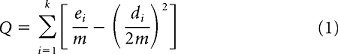
Figure 5.

Large spheres represent the COM of the 12 clusters of modules. The COM of these clusters is the mean of the COM of the modules that constitute each cluster. Small spheres represent the COM of the modules of each cluster detected for each subject (see also Fig. 3). Only group representative clusters are depicted that contain modules from at least 7 of 12 subjects. Each sphere has a unique color, and the COM of modules belonging to the same cluster are the same color.

LFC families

Quantification of the similarity of the whole-brain FC of the clusters of modules resulted in four families, organized across the dorsal–ventral and anterior–posterior axes (Fig. 6). The degree of similarity within and between the families is also evident in the raw pairwise whole-brain FC similarities of the clusters of modules constituting each family (Fig. 6A). Both clustering techniques (hierarchical and k-means) identified the same four families (Fig. 6B,C). The dendrogram obtained from the hierarchical clustering (Fig. 6B) corresponds to a cophenetic correlation coefficient of 0.685; hence, it does not severely distort the original distances of the raw data. With respect to the k-means clustering, the highest silhouette (0.693) for non-singleton solutions was observed for k = 4, corresponding to the same families traced by the hierarchical clustering (Fig. 6C). Solutions for k = 2 and 3 gave rise to silhouette values of 0.540 and 0.563 respectively. Solutions for k > 4 contained singletons and thus were not taken into account. Moreover, the traced families always constituted a family across 1000 solutions, as indicated by the frequency of the co-clustering matrix, which is dominated exclusively by entries with a value of 0 (never co-clustered) or 100 (always co-clustered) (Fig. 6C), illustrative of the robustness of the findings. Taken together, the above results highlight the presence of four distinct families within the LFC, organized across the dorsal–ventral and anterior–posterior axes, which can be differentiated through their whole-brain FC. This differentiation is also evident in the FC maps of the clusters of modules constituting each family (Fig. 7).

Figure 6.

A, Representation of the raw similarity of the whole-brain FC among the traced clusters of modules. Clusters are arranged in space by using the Kamada–Kawai spring-embedding algorithm, based on the similarity of their whole-brain FC. Thick (thin) lines indicate high (low) similarity, and circles delineate the families traced with hierarchical and k-means clustering. B, Dendrogram representing the similarity of the whole-brain FC of the cluster of modules. Each brain depicts the COM of the clusters of modules that form a family (i.e., have similar whole-brain FC). A set of clusters of modules formed a family if the “intrafamily” distance was less than the 70% of the largest distance in the dendrogram. C, Clusters of modules grouped according to their whole-brain FC similarity with the k-means algorithm. Brackets denote the grouping of the clusters of modules to families. The frequency of the co-clustering matrix indicates the high stability of the families across 1000 k-means solutions (see Materials and Methods and Results for details). The color coding for each cluster of modules follows that of Figure 5.

Figure 7.

Whole-brain FC of the 12 clusters of modules grouped according to the four LFC families. Clusters are grouped according to the LFC family to which they belong (see Fig. 6) following the color coding of Figure 5. Darker (violet/red) regions represent higher t values. All maps are thresholded at q < 0.05 (FDR level). Note the FC similarities (or dissimilarities) among clusters of modules that belong to the same (or different) family. For the computation of these second level maps, different ROIs derived from the parcellation obtained from each subject were used (see Materials and Methods).

A family located at the ventral part of the LFC was formed from the clusters of modules located across the IFS (C3, C5, C11, C12). These regions exhibit FC with regions that are part of the multiple demand/frontoparietal network recruited in various cognitive tasks (Fig. 7) (Vincent et al., 2008; Duncan, 2010; Stiers et al., 2010). The clusters located at the more dorsal parts of the LFC (C6, C10) formed a family with a “default mode” signature (Fig. 7) associated with internal processes (Buckner et al., 2008). The cluster of modules likely to correspond to region 46 (C8) (see Cluster documentation) formed a family with the more posterior clusters (C1, C7, C9), with a premotor/occulomotor signature (Fig. 7), and not the immediately adjacent more anterior ones (e.g., modules of C3, C10). This likely reflects the assumed role of region 46 in high levels of motor control (Goldman-Rakic, 1987) (see Discussion). Finally, the more anterior clusters, C2 and C4, also formed a family exhibiting FC with the temporal cortex and the medial wall (Fig. 7) and are possibly implicated in audiovisual and semantic processing (see Discussion).

Interestingly, the families do not seem completely constrained by Euclidean distance—that is, the clusters of modules of the same family—can be remote from one another. For instance, C8 is located more anterior than the rest of the clusters of the family to which it belongs (Fig. 6). Hence, subregions with similar whole-brain FC can be dispersed throughout the LFC (Yeo et al., 2011).

Cluster comparisons

C1 versus C2.

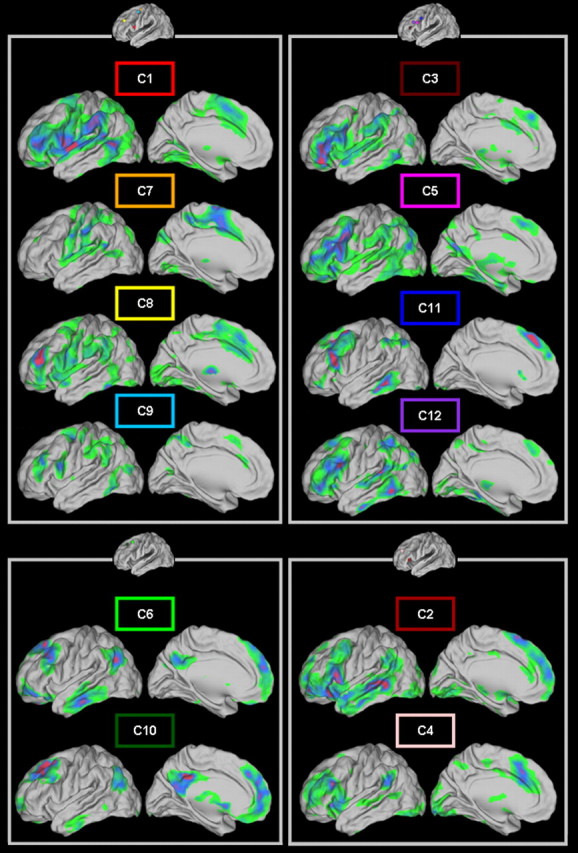
Direct comparisons between the FC associated with C1 and C2 revealed significant differences. C1 exhibited more pronounced FC with the anterior part of the supramarginal gyrus (SMG), the intraparietal sulcus (IPS), the anterior part of the IFS, the medial part of the insula, the junction of the IFS with the SFS, and the supplementary motor area (SMA). C2 exhibited more pronounced FC with the anterior medial PFC, the angular gyrus (AG), the anterior temporal cortex, and the posterior cingulate cortex (PCC) (Figs. 7, 8A).

Figure 8.

A–C, Direct comparisons through t tests reveal significant differences in the whole-brain FC of clusters located at the ventral (A, B) and dorsal (C) parts of the LFC. Significant differences associated with a particular cluster follow the color coding in Figure 5. Maps depict regions that are significant at q < 0.05 (FDR level).

C2 versus C3.

The direct contrast between C3 and C2 revealed higher FC of C2, with the triangular and orbital part of the IFG and the middle temporal cortex. Moreover, higher FC was observed with the SFG extending toward the medial wall. C3 showed pronounced higher FC with the IFS with an extension toward the junction with the prCS, the junction of the SFS and the prCS, the anterior and posterior SMG, the IPS with an extension toward the occipital lobes, and the mid-cingulate cortex (MCC) (Figs. 7, 8B).

C9 versus C6 and C10.

Direct comparisons of the FC of C9 with C6 and C10 revealed pronounced differences. C9 compared to C10 was more functionally connected with the ventral prCS, the dorsolateral PFC, the IPS, and parts of the occipital–parietal cortex (involving higher visual areas). Moreover, pronounced FC was observed with the anterior insula, the SMA, and the cingulate motor regions (CMRs) in the MCC and parts of the postero-medial cortex likely to include Brodmann's region 7. The immediately adjacent C10, located anterior to C9, exhibited higher FC with the posterior part of the middle frontal gyrus (MFG), the AG, the SFG, the anterior medial PFC with parts of the anterior cingulate cortex (ACC), the limbic region PCC, and the orbitofrontal cortex (Figs. 7, 8C). A very similar pattern of FC differences emerged when C9 was compared to adjacent C6 (data not shown).

These FC differences of adjacent clusters at the ventral and dorsal parts of the LFC are consistent with observations of structural connectivity and FC in the human brain (Frey et al., 2008; Vincent et al., 2008; Ford et al., 2010) and connectivity of suggested homologs in the monkey brain (Pandya and Yeterian, 1996; Petrides and Pandya, 2009). They illustrate the FC differences, which are also observable in Figure 7, that might relate to the different functional specializations associated with the subregions of each cluster (see Discussion).

Cluster documentation

In this section we will assign a potential anatomical substrate to each cluster. To this end, macroscopic landmarks, cytoarchitectonic maps, and the whole-brain FC of each cluster will be used in combination with known structural connectivity and FC of subregions of the human brain and candidate homologues in the macaque brain. The results reported concern the left hemisphere.

C1.

The COM of the cluster is located anterior to the ventral part of the premotor cortex, in the depths of the prCS (Fig. 5). The modules of this cluster occupy the prCS and extend toward the opercular part of the IFG (Figs. 3B, red modules, 9A,B). The coordinates of the COM are very near to the ones reported from a Diffusion Weighted Imaging (DWI)-based parcellation of BA 44 (Anwander et al., 2007) and a couple of millimeters caudally to the ROI used in an rsfMRI study investigating the FC of BA 44 (Kelly et al., 2010) (Table 1). In addition, the COM falls within the region of the probabilistic map of BA 44 that exhibits high probability (Amunts et al., 1999) (Fig. 9B). The FC map of C1 unveils extensive FC with regions located ventral to the IFS (Fig. 7). Extensive FC of C1 was observed with pre-SMA, SMA, and the anterior MCC. Evidence from tracing studies suggests that region 44 in the macaque is connected with assumed homolog, more specifically with dorsal region MII, caudal 24, and the CMR (Pandya and Yeterian, 1996; Paus, 2001; Pickard and Strick, 2001). Moreover, a recent DWI study in humans also reveals structural connections of the posterior part of Broca's region (region 44) with SMA and preSMA, in contrast, the anterior part (region 45), which is anatomically linked with more anterior parts of the medial wall (Ford et al., 2010). Concerning the post-rolandic regions, prominent FC involved a big portion of the SMG, in line with the connectivity of assumed homologs in the monkey brain (Petrides and Pandya, 2009, 2004). Last, FC was also observed with the IPS. This is consistent with evidence from the connectivity of the monkey brain (Petrides and Pandya, 2009). In addition, tracts connecting region 44 and the IPS have been traced in the human brain with DWI (Frey et al., 2008).

Figure 9.

A–D, Variability maps of the clusters of modules across subjects. A, Cortical patches indicating the overlap of the clusters of modules across subjects. Each cortical patch denotes the extent of the variability (thresholded at 60%) of each cluster of modules. The color coding scheme is the same as the rest of the figures; white denotes the intersection of cortical patches. B, Variability maps for C1 and C2 (putative BA 44 and 45, respectively). Variability maps of FC based parcellation (left) are depicted along with variability maps from cytoarchitectonic based parcellation of putative BAs (right). Cytoarchitectonic maps are part of the SPM anatomy toolbox (Eickhoff et al., 2005). Variability maps for C, C8 (putative BA 46) and D, C10 (putative (lateral) BA 9). C, D, Bounding boxes define conservative estimates of the location of BAs 46 and 9. These conservative estimates are derived from a cytoarchitectonic-based parcellation (Rajkowska and Goldman-Rakic, 1995). Coordinates for the formation of the bounding boxes were approximated through a conversion from Talairach to MNI space. B–D, Variability maps are unthresholded; bright yellow indicates higher overlap across subjects. Note the good correspondence between FC and cytoarchitectonic-based parcellation.

C2.

Modules belonging to this cluster occupy the triangular part of the IFG associated with BA 45 (Amunts et al., 1999) (Figs. 3A, dark red module, 9A,B). The COM of this cluster (Fig. 5) is located within the probabilistic map of BA 45 (Fig. 9B) and is close to the COM of a region identified as BA 45 in a DWI-based parcellation (Anwander et al., 2007) and the coordinates of an ROI used to trace the FC of BA 45 (Kelly et al., 2010) (Table 1). C2 exhibited extensive FC with a large part of the LFC (Fig. 7). With respect to regions outside the LFC, FC was pronounced with the lateral temporal lobe, the anterior part of the medial prefrontal wall and parts of the ACC, and the posterior SMG extending toward the AG. The FC of C2 resembles the connectivity of the assumed homolog of region 45 in the monkey brain. More precisely, strong connections of macaque region 45 exist with various visual, auditory, and multimodal areas located at the temporal cortex (Pandya and Yeterian, 1996; Petrides and Pandya, 2009; Gerbella et al., 2010). Tracers have also revealed connectivity of region 45 with area PFG in the macaque, which is the assumed homolog of the posterior part of the SMG in the human brain (Petrides and Pandya, 2009). Prominent connectivity of region 45 in the macaque has also been reported with the anterior part of the medial wall (Pandya and Yeterian, 1996). Interestingly, in line with the results of our study, a recent DWI study in humans revealed a posterior-to-anterior gradient with respect to the connectivity of Broca's regions (regions 44 and 45) and the medial wall, with region 45 exhibiting structural connectivity with anterior parts of the medial wall (Ford et al., 2010).

C3.

The COM of this cluster is located at the most anterior part of the IFS, dorsal to the triangular part of the IFG (Fig. 5). Modules belonging to this cluster are located at the tip of the IFS, extending dorsally toward the MFG and ventrally toward the IFG (Figs. 3D, brown modules, 9A). Different cytoarchitectonic parcellation schemes have labeled differently the region adjacent to the dorsal part of the pars triangularis. In Brodmann's map, this part of the cortex is labeled region 46, whereas in Sarkissov et al. (1955), this part is labeled region 9 (Fig. 1A,B). Regions 46 and 9 exhibit considerable interindividual variability, which, along with the presence of many transitional zones with mixed cytoarchitectonic features, can contribute to the diversity of the various parcellation schemes (Rajkowska and Goldman-Rakic, 1995). In the later study, transition zones referred to as 46–45, 9–45 were observed at the fundus of the IFS dorsal to region 45, which resembles the position at which C3 is located. Moreover, this patch of the cortex might correspond to the most anterior tip of region 9/46v of the Petrides and Pandya (1994) parcellation (Fig. 1C). C3 exhibits FC mainly with the IPS, extending toward the parieto-occipital complex and the SMG. Extensive FC was also observed with the ventrolateral prefrontal cortex, IFS, the preSMA, and MCC (with parts of the CMR) (Fig. 7). Interestingly, a distinct cluster located dorsally to BA 45, extending across the IFS and exhibiting similar FC, was traced in an rsfMRI-based parcellation (Kelly et al., 2010).

C4.

The COM of the cluster is located most anterior to any other clusters identified (Fig. 5). The modules constituting this cluster extend around the pragmatical posterior border for the frontal pole proposed by Uylings et al. (2010) (Figs. 3A, light pink modules, 9A). Consequently, it seems the case that the identified modules of this cluster correspond to bits of the lateral frontopolar cortex (i.e., region 10) (Fig. 1A). It exhibits FC with the anterior of MCC and the posterior of SMG (Fig. 7).

C5.

The COM of this cluster is located at the IFS before the junction with the prCS, dorsal to the triangular and opercular parts of the IFG (Fig. 5). The cluster consists of modules that primarily occupy the fundus of the IFS (Figs. 3C, fuchsia module, 9A). The position of the modules corresponds to the cortical region labeled region 9 (Sarkissov et al., 1955) (Fig. 1B) and to transitional zones of region 9 (Rajkowska and Goldman-Rakic, 1995). Parcellation schemes that exploit the mixed cytoarchitectonic features of these transitional zones of region 9 have labeled this part of the cortex region 9/46v (Petrides and Pandya, 1994) (Fig. 1C). Extensive FC was observed with regions that are implicated in the execution of diverse tasks (Duncan, 2010) and are part of a network unveiled with rsfMRI termed the frontoparietal control network (Vincent et al., 2008) (Fig. 7).

C6.

The COM of this cluster is located at the posterior part of the MFG (Fig. 5). The modules that constitute this cluster occupy the most posterior part of the MFG (Figs. 3C, light green module, 9A). This part of the cortex is labeled region 8, and it has as an anterior border region 9 (Brodmann, 1909; Sarkissov et al., 1955) (Fig. 1A,B). Cytoarchitectonic and variability analysis of region 9 indicates that the vertical plane located at y = +26 (approximate coordinate in MNI space) can function as a conservative posterior limit of region 9 (Rajkowska and Goldman-Rakic, 1995). The identified modules of this cluster extent predominantly posterior to this plane. Moreover, the parcellation scheme of Petrides and Pandya (1994) labels the part of the cortex where the modules are located region 8, more specifically, region 8Ad (Fig. 1C). C6 exhibits extensive FC with the AG, the anterior medial wall and ACC, the orbital part of the IFG, the inferior temporal sulcus, and the PCC (Fig. 7). This FC map is very similar to the one characteristic of the so-called default mode network (Buckner et al., 2008).

C7.

The COM of this cluster is located at the precentral gyrus and constitutes the most posterior cluster (Fig. 5). The modules constituting this cluster are primarily localized in parts of the cortex that exhibit high probability of belonging to region 6 (Geyer, 2004) (Figs. 3A, orange module, 9A). The FC map of C7 includes large parts of the premotor and motor cortex and is similar to maps derived from seed-based approaches that involve motor-related regions such as the SMA (Kim et al., 2010) and the posterior MCC (Fig. 7). Thus, it seems that modules that are part of this cluster correspond to bits of premotor regions in the most posterior part of the LFC mask.

C8.

The COM of this cluster is located at the anterior part of the MFG (Fig. 5). The modules that constitute this cluster consistently occupy the convolutions of the anterior part of the MFG, with an occasional very moderate extension toward the SFS and the IFS (Figs. 3A, yellow module, 9A,C). The position of the modules corresponds well with the location of region 46, delineated according to cytoarchitectonic properties, and falls within conservative boundaries specified for this region (Rajkowska and Goldman-Rakic, 1995) (Fig. 9C). Moreover, other cytoarchitectonic parcellation schemes also label this part of the prefrontal cortex region 46, despite differences in the exact extent and shape of the region (Brodmann, 1909; Sarkissov et al., 1955; Petrides and Pandya, 1994) (Fig. 1). C8 exhibits extensive FC with various parietal (SMG, IPS), prefrontal (IFS), and premotor and medial regions (MCC, SMA, preSMA, CMR, ventral premotor) (Fig. 7). This diffuse pattern of FC might give rise to the role that this region seems to play in diverse aspects of motor control and higher order processes (Goldman-Rakic, 1987; Lu et al., 1994; Petrides, 2005).

C9.

This cluster consists of modules located near the junction of the SFS with the prCS (Figs. 3C, cyan modules, 9A). The junction of the prCS with the SFS has been identified as the locus of the frontal eye fields (FEFs) in the human brain (Koyama et al., 2004). Its COM (Fig. 5) is very near reported peaks of task-induced activations involving a goal-directed visual search of a target stimulus (Asplund et al., 2010) attending, pointing, and looking at a peripheral visual location (Astafiev et al., 2003) (Table 1). Moreover, the location of the modules belonging to this cluster is also consistent with the region that has been localized as the human FEF via electrical cortical stimulation (Blanke et al., 2000). It should be noted, however, that within this region there might be functional subspecializations, as suggested by the presence of visuospatial maps (Hagler et al., 2007). C9 is located anterior to C7, which exhibits a more motor-related FC and posterior to clusters 6 and 10, which occupy portions of the posterior MFG and the SFS, respectively. Hence, C9 is located between portions of cortex most likely belonging to the anterior premotor cortex (BA 6) and portions of cortex that could correspond to regions 9, 9–46 (Rajkowska and Goldman-Rakic, 1995) and 8Ad, 9–46d (Petrides and Pandya, 1994) (Fig. 1C). The FC map of C9 is highly similar to the FC map that is obtained by seeding from the FEF (Fox et al., 2006) and to the map corresponding to the dorsal attention system of which the FEF constitutes a core region (Vincent et al., 2008) (Fig. 7). This set of regions is similar to the network involved in smooth eye pursuit and saccades in the monkey brain (Tian and Lynch, 1996).

C10.

The COM of this cluster is located more anterior and dorsal to the COM of C6 (Fig. 5). The modules of C10 extend across the SFS, occupying its fundus (Figs. 3A, dark green module, 9A,D). The anatomical location of the modules matches the location of (lateral) region 9 and the transition zone 9–46, with the largest part of the modules falling within the conservative boundaries of region 9 (Rajkowska and Goldman-Rakic, 1995) (Fig. 9D). Other cytoarchitectonic parcellation schemes label this part of the cortex region (lateral) 9, 9/46d (Petrides and Pandya, 1994) (Fig. 1C). The FC map of C10 was very similar to the FC map of C6, resembling the default mode network, and it encompasses parts of the PCC/retrosplenial cortex, dorsal and ventral medial PFC, ACC, AG, SFS, and ventral temporal cortex (Fig. 7). This FC pattern resembles connectivity, as revealed by tracer studies, involving assumed homologs of region 9/46d in the monkey brain (Pandya and Yeterian, 1996).

C11.

The COM of this cluster is located dorsal to the COM of C1 (Fig. 5). The modules occupy the meeting point of the IFS and the prCS (Figs. 3A, blue module, 9A). Different cytoarchitectonic parcellation schemes label this part of the cortex differently. In Brodmann's map this part of the prefrontal cortex is labeled region 9 (Fig. 1A). According to Sarkissov et al. (1955), the region adjacent to the dorsal part of region 44 is labeled region 8 (Fig. 1B). Other parcellation schemes exploit cytoarchitectonic inhomogeneities of region 8 and introduce further subdivisions (Petrides and Pandya, 1994) (Fig. 1C). According to the latter parcellation, the region adjacent dorsal to area 44 is labeled 8Av. The modules of C11 in our study do not resemble region 9 since they do not extend toward the superior frontal gyrus nor do they follow the pattern of region 8. Instead they have a location and spatial extent similar to those of region 8Av according to the Petrides and Pandya (1994) parcellation (Fig. 1C). FC for C11 was observed with regions located ventrally (across the IFG) and dorsally (in the posterior part of the MFG extending to the posterior fundus of the SFS). FC was also observed with the IPS extending toward the AG, with the dorsal anterior MCC and with the temporal region just anterior to the MT+ complex (Fig. 7). It is interesting to note that the position of the modules of C11 is at the vicinity of the recent functionally defined region termed the inferior frontal junction (Brass et al., 2005) and is recruited during diverse cognitive tasks (Stiers et al., 2010). This region has also been demonstrated to exhibit distinct recepto- and cyto-architectonic properties (Amunts et al., 2004b).

C12.

The COM of this cluster is located anterior to the COM of C5 (Fig. 5). The modules constituting this cluster are located dorsal to the triangular/opercular part of the IFG (Figs. 3D, violet module, 9A). The possible anatomical correlates resemble the ones described for C5. Its FC is also very similar with the FC of C5 (Fig. 7).

The fact that C5 and C12 seem to correspond to the same cytoarchitectonic substrate might reflect functional subdifferentiations within cytoarchitectonically homogeneous regions. This is in line with deviations from a 1:1 relation of cytoarchitectonic- and receptor-, closely linked with functional aspects, based parcellations (Zilles and Amunts, 2011). Interestingly, task-based paradigms (Badre and D' Esposito, 2009; Stiers et al., 2011) and receptor mapping (Amunts et al., 2010) support the presence of separate regions across the IFS (possibly corresponding to region 9/46v). The investigation of these issues and the differences between functional subdivisions of regions 9/46v can constitute the topic of future studies.

Discussion

In the current study we delineated in vivo and on an individual basis subregions of the LFC with the aid of rsfMRI and data-driven algorithms. The subregions traced at the individual level were grouped with a data-driven, across-subjects clustering, allowing the examination of the subregions at the group level, which is a step forward from observer-dependent approaches (Barnes et al., 2010).

Ventral and dorsal LFC clusters

Subregions of the ventral LFC that seem to correspond to cytoarchitectonic divisions, namely regions 44 (C1) and 45 (C2) (i.e., Broca's regions) and transitional zones 46–45, 9–45 (C3) (Rajkowska and Goldman-Rakic, 1995; Amunts et al., 1999) exhibit distinct FC, placing them into different families (Figs. 6, 7).

C1 and C2 show FC differences consistent with distinct connectivity patterns of assumed homologs in the monkey (Pandya and Yeterian, 1996) and structural connections in the human brain (Frey et al., 2008; Ford et al., 2010) (see Results and Fig. 8A) that can account for separate functional roles in the language domain. Region 44 is involved in a neural circuitry responsible for hand and orofacial control and generation of speech acts (Petrides et al., 2005; Ford et al., 2010). Region 45 is connected with multimodal, auditory, and visual areas (Pandya and Yeterian, 1996; Gerbella et al., 2010) and is involved in semantic, audiovisual processing, and emotional embedding of auditory stimuli (Barbas, 2000; Amunts et al., 2004a; Gerbella et al., 2010).

C2 and C3 show significant FC differences (Fig. 8B). Cytoarchitectonic analysis of region 45 (C2) indicates its occasional extension toward the ventral and dorsal banks of the IFS (Amunts et al., 1999). Cytoarchitectonic and receptor mapping studies pinpoint a separate region at the IFS, termed transition zone 46–45, 9–45 (Rajkowska and Goldman-Rakic, 1995) and ifs1 (Amunts et al., 2010). The current parcellation is consistent with these studies, suggesting the presence of a subregion (C3) occupying the IFS, dorsal to the triangular IFG, with a distinct FC pattern from the one of region 45 (C2), involving a neural circuitry spanning visuospatial and sensory-occulomotor regions (Fig. 8B).

Subregions of the dorsal LFC seem to correspond to FEF (C9) and to regions 8Ad (C6) and lateral 9, 9/46d, 9–46 (C10) (Petrides and Pandya, 1994; Rajkowska and Goldman-Rakic, 1995; Koyama et al., 2004) and belong to different families (Fig. 6).

Comparison of the FC of C9, located at the junction of the SFS and the prCS, to C10, located at the fundus of the SFS, reveals FC with regions of the dorsal attention system (Fox et al., 2006) (Fig. 8C) involved in externally guided attention and occulomotor functions (Barbas, 2000; Corbetta et al., 2008). Comparison of the FC of C10 to C9 reveals FC with regions of the default network (Fig. 8C) involved in “internal” processes such as episodic memory retrieval (Raichle et al., 2001; Buckner et al., 2008). Similar FC differences emerge when contrasting the FC of C9 and C6 (data not shown). The above illustrate the transition of whole-brain FC along the anterior–posterior axis at the dorsal LFC, involving distinct subregions belonging to different large-scale networks that obey a broad “externally/internally oriented” dichotomy (Vincent et al., 2008).

LFC families and FC with the cingulate cortex

Based on receptor profiles, the cingulate cortex can be divided into three gross parts (Palomero-Gallagher et al., 2009) also characterized by functional specializations (Beckman et al., 2009): ACC, MCC, and PCC/retrosplenial. Interestingly, the different LFC families exhibit preferential FC with different cingulate divisions.

C6 and C10 exhibit FC with the PCC/retrosplenial and ACC (Fig. 7). The PCC is associated with memory tasks (Beckman et al., 2009) and, compared to more anterior divisions, exhibits higher densities of acetylcholine, which is implicated in memory formation (Miranda et al., 2003; Palomero-Gallagher et al., 2009). The ACC is associated with processes such as mentalizing, linked with the default mode network (Amodio and Frith, 2006; Buckner et al., 2008). C3, C5, C11, and C12, which correspond to regions engaged in diverse cognitive tasks (Duncan, 2010), exhibit FC only with MCC, mostly with its anterior part (Fig. 7), and not the ACC and PCC/retrosplenial. MCC is associated with cognitive and—mostly its posterior part, exhibiting high GABA_B densities resembling motor regions—motor tasks (Ridderinkhof et al., 2004; Beckman et al., 2009; Palomero-Gallagher et al., 2009). The family formed from C1 and C7–C9, which are linked to motor/occulomotor processes (see Results), exhibits FC only with the MCC, encompassing it almost entirely, including its more posterior part (Fig. 7). Last, C2 and C4 exhibit FC with anterior MCC and the ACC (Fig. 7), which might relate to functions in the language domain.

Thus, the neural circuitry of each LFC family also encompasses distinct specialized cingulate divisions that correspond to the functional roles attributed to the LFC families (Barbas, 2000; Amunts et al., 2004a; Buckner, 2008; Duncan, 2010).

Region 46 and motor control

Interestingly C8 (i.e., presumed region 46) formed a family with the most posterior LFC clusters. C8 exhibits FC with the SMA, preSMA, the ventral premotor cortex, and the CMR (see Results) (Figs. 6, 7), resembling connections among assumed macaque homologs (Goldman-Rakic, 1987; Lu et al., 1994; Barbas, 2000; Pickard and Strick, 2001). This connectivity pattern, along with additional functions of region 46 such as the integration of goals maintained on-line and visuospatial information, can render possible the coordination of movement (Goldman-Rakic, 1987; Lu et al., 1994). The LFC family to which C8 belongs, its extensive and diffuse FC with premotor/occulomotor and visuospatial regions (Fig. 7), suggests that in the human brain there is a relative perseverance of the neural circuitry present in the monkey brain, involving region 46, wherein the latter seems involved in high levels of motor behavior.

Relation to LFC models

The organization and FC of the LFC families along the anterior–posterior and dorsal–ventral axis partially comply with previous LFC models (Petrides, 2005). The dorsal family (C6, C10) exhibits FC with the PCC/retrosplenial cortex through which access to memory-related structures is accomplished (Fig. 7) (Morris et al., 1999). The ventral family (C3, C5, C11, C12) is involved in a functional circuitry spanning audiovisual and somatomotor regions at the parietal and temporal cortexes (Fig. 7). The posterior family (C1, C7-C9) includes regions involved in response selection and stimulus–response mappings (Corbetta et al., 2008; Badre and D'Esposito, 2009). However, members of this family are not constrained by Euclidean distance, and, despite that C8 is located at mid-dorsal LFC, it does not exhibit similar whole-brain FC with its spatially adjacent subregions (Petrides, 2005). Instead it is affiliated with premotor regions, consistent with proposed LFC models (Miller and Cohen, 2001). The violation of a strict ordering according to Euclidean distance seemingly contradicts models advocating a hierarchical anterior–posterior gradient (Badre and D'Esposito, 2009). However, these models are compatible with the traced families since regions with a similar functional circuitry might be differentiated through their oscillation frequency (Baria et al., 2011), which is related to integrative capacities (Von Stein and Sarnthein, 2000) and/or the degree of rule abstraction and regulatory effective connectivity (Koechlin et al., 2003). Interestingly, the regions of the Koechlin model approximately coincide with the ones constituting a family (C1, C7-C9), with C8, also involved in high-order mechanisms of motor control, located more anterior than the rest, consistent with a potential hierarchical anterior–posterior gradient. A combination of rsfMRI-based parcellation and task-based paradigms can further inform the various LFC models.

Limitations and caveats

The resolution limit inherent in the module detection algorithm used constrains the number of modules that can be resolved (Fortunato and Berthelemy, 2007). Consequently, the modules obtained might be further subdivided. For instance, further subdivision of modules corresponding to presumed region 45 may reveal the anatomical subdivisions of this region (Amunts et al., 1999). Advances in network analysis might be used to overcome the resolution limit (Ruan and Zhang, 2008). Moreover, the limited spatial resolution and preprocessing steps can lead to “signal bleeding” to adjacent regions. For instance, modules of C1 (region 44) can extend posterior to the prCS (Fig. 3D), contrary to evidence from cytoarchitectonic studies. A parcellation that incorporates cortical distance information and higher acquisition resolution might ameliorate the results.

Conclusions

The present study unravels the intrinsic functional organization of the LFC. With rsfMRI we could trace neuroanatomically realistic LFC subregions and elucidate their distinct FC patterns that could segregate them into families. This segregation seems related to functional specializations (Passingham et al., 2002) and reflects the view that the LFC is a constellation of specialized information-processing systems (Miller, 2000). Similarities with known connectivity of assumed LFC monkey homologs were observed despite differences due to expansion and/or rewiring (Semendeferi et al., 2002; Van Essen and Dierker, 2007), extending and complying with recent evidence and LFC models (Petrides, 2005; Kelly et al., 2010; Petrides et al., 2011). Future comparative studies will offer a closer interspecies comparison. The current parcellation can guide and be complemented by other studies focusing on the LFC that could examine task-related properties and potential interhemispheric differences. Last, the methods used can be the basis for preoperative neurosurgery mapping.

References

- Amodio DM, Frith CD. Meeting of minds: the medial frontal cortex and social cognition. Nat Rev Neurosci. 2006;7:268–277. doi: 10.1038/nrn1884. [DOI] [PubMed] [Google Scholar]
- Amunts K, Schleicher A, Bürgel U, Mohlberg H, Uylings HB, Zilles K. Broca's region revisited: cytoarchitecture and intersubject variability. J Comp Neurol. 1999;412:319–341. doi: 10.1002/(sici)1096-9861(19990920)412:2<319::aid-cne10>3.0.co;2-7. [DOI] [PubMed] [Google Scholar]
- Amunts K, Weiss PH, Mohlberg H, Pieperhoff P, Eickhoff S, Gurd JM, Marshall JC, Shah NJ, Fink GR, Zilles K. Analysis of neural mechanisms underlying verbal fluency in cytoarchitectonically defined stereotaxic space-the roles of Brodmann areas 44 and 45. Neuroimage. 2004a;22:42–56. doi: 10.1016/j.neuroimage.2003.12.031. [DOI] [PubMed] [Google Scholar]
- Amunts K, Palomero-Gallagher N, Brass M, Derrfuss J, Zilles K, Cramon DYV. A receptor and cytoarchitectonic correlate of the functionally defined inferior-frontal junction area. Neuroimage. 2004b;22(Suppl):50. [Google Scholar]
- Amunts K, Lenzen M, Friederici AD, Schleicher A, Morosan P, Palomero-Gallagher N, Zilles K. Broca's region: novel organizational principles and multiple receptor mapping. PLoS Biol. 2010;8:e1000489. doi: 10.1371/journal.pbio.1000489. [DOI] [PMC free article] [PubMed] [Google Scholar]
- Anwander A, Tittgemeyer M, von Cramon DY, Friederici AD, Knösche TR. Connectivity-based parcellation of Broca's area. Cereb Cortex. 2007;17:816–825. doi: 10.1093/cercor/bhk034. [DOI] [PubMed] [Google Scholar]
- Asplund CL, Todd JJ, Snyder AP, Marois R. A central role for the lateral prefrontal cortex in goal-directed and stimulus-driven attention. Nat Neurosci. 2010;13:507–512. doi: 10.1038/nn.2509. [DOI] [PMC free article] [PubMed] [Google Scholar]
- Astafiev SV, Shulman GL, Stanley CM, Snyder AZ, Van Essen DC, Corbetta M. Functional organization of human intraparietal and frontal cortex for attending, looking, and pointing. J Neurosci. 2003;23:4689–4699. doi: 10.1523/JNEUROSCI.23-11-04689.2003. [DOI] [PMC free article] [PubMed] [Google Scholar]
- Badre D, D'Esposito M. Functional magnetic resonance imaging evidence for a hierarchical organization of the prefrontal cortex. J Cogn Neurosci. 2007;19:2082–2099. doi: 10.1162/jocn.2007.19.12.2082. [DOI] [PubMed] [Google Scholar]
- Badre D, D'Esposito M. Is the rostro-caudal axis of the frontal lobe hierarchical? Nat Rev Neurosci. 2009;10:659–669. doi: 10.1038/nrn2667. [DOI] [PMC free article] [PubMed] [Google Scholar]
- Barbas H. Proceedings of the human cerebral cortex: From gene to structure and function. Connections underlying the synthesis of cognition, memory, and emotion in primate prefrontal cortices. Brain Res Bull. 2000;52:319–330. doi: 10.1016/s0361-9230(99)00245-2. [DOI] [PubMed] [Google Scholar]
- Baria AT, Baliki MN, Parrish T, Apkarian AV. Anatomical and functional assemblies of brain BOLD oscillations. J Neurosci. 2011;31:7910–7919. doi: 10.1523/JNEUROSCI.1296-11.2011. [DOI] [PMC free article] [PubMed] [Google Scholar]
- Barnes KA, Cohen AL, Power JD, Nelson SM, Dosenbach YB, Miezin FM, Petersen SE, Schlaggar BL. Identifying basal ganglia divisions in individuals using resting-state functional connectivity MRI. Front Syst Neurosci. 2010;4:18. doi: 10.3389/fnsys.2010.00018. [DOI] [PMC free article] [PubMed] [Google Scholar]
- Barnes KA, Nelson SM, Cohen AL, Power JD, Coalson RS, Miezin FM, Vogel AC, Dubis JW, Church JA, Petersen SE, Schlaggar BL. Parcellation in left lateral parietal cortex is similar in adults and children. Cereb Cortex. 2012;22:1148–1158. doi: 10.1093/cercor/bhr189. [DOI] [PMC free article] [PubMed] [Google Scholar]
- Beckmann M, Johansen-Berg H, Rushworth MF. Connectivity-based parcellation of human cingulate cortex and its relation to functional specialization. J Neurosci. 2009;29:1175–1190. doi: 10.1523/JNEUROSCI.3328-08.2009. [DOI] [PMC free article] [PubMed] [Google Scholar]
- Blanke O, Spinelli L, Thut G, Michel CM, Perrig S, Landis T, Seeck M. Location of the human frontal eye field as defined by electrical cortical stimulation: anatomical, functional and electrophysiological characteristics. Neuroreport. 2000;11:1907–1913. doi: 10.1097/00001756-200006260-00021. [DOI] [PubMed] [Google Scholar]
- Blondel VD, Guillaume JL, Lefebvre E. Fast unfolding of communities in large networks. J Stat Mech. 2008:P10008. [Google Scholar]
- Brass M, Derrfuss J, Forstmann B, von Cramon DY. The role of the inferior frontal junction area in cognitive control. Trends Cogn Sci. 2005;9:314–316. doi: 10.1016/j.tics.2005.05.001. [DOI] [PubMed] [Google Scholar]
- Brodmann K. Vergleichende Localisationslehre der Grosshirnrinde in ihren Prinzipien dargestellt auf Grund des Zellenbaues. Leipzig: Barth; 1909. [Google Scholar]
- Buckner RL, Andrews-Hanna JR, Schacter DL. The brain's default network: anatomy, function, and relevance to disease. Ann NY Acad Sci. 2008;1124:1–38. doi: 10.1196/annals.1440.011. [DOI] [PubMed] [Google Scholar]
- Cohen AL, Fair DA, Dosenbach NU, Miezin FM, Dierker D, Van Essen DC, Schlaggar BL, Petersen SE. Defining functional areas in individual human brains using resting functional connectivity MRI. Neuroimage. 2008;41:45–57. doi: 10.1016/j.neuroimage.2008.01.066. [DOI] [PMC free article] [PubMed] [Google Scholar]
- Corbetta M, Patel G, Shulman GL. The reorienting system of the human brain: from environment to theory of mind. Neuron. 2008;58:306–324. doi: 10.1016/j.neuron.2008.04.017. [DOI] [PMC free article] [PubMed] [Google Scholar]
- Cordes D, Haughton VM, Arfanakis K, Wendt GJ, Turski PA, Moritz CH, Quigley MA, Meyerand ME. Mapping functionally related regions of brain with functional connectivity MR imaging. Am J Neuroradiol. 2000;21:1636–1644. [PMC free article] [PubMed] [Google Scholar]
- De Luca M, Beckmann CF, De Stefano N, Matthews PM, Smith SM. fMRI resting state networks define distinct modes of long-distance interactions in the human brain. Neuroimage. 2006;29:1359–1367. doi: 10.1016/j.neuroimage.2005.08.035. [DOI] [PubMed] [Google Scholar]
- Doucet G, Naveau M, Petit L, Delcroix N, Zago L, Crivello F, Jobard G, Tzourio-Mazoyer N, Mazoyer B, Mellet E, Joliot M. Brain activity at rest: a multi-scale hierarchical functional organization. J Neurophysiol. 2011;105:2753–2763. doi: 10.1152/jn.00895.2010. [DOI] [PubMed] [Google Scholar]
- Duncan J. The multiple-demand (MD) system of the primate brain: mental programs for intelligent behaviour. Trends Cogn Sci. 2010;14:172–179. doi: 10.1016/j.tics.2010.01.004. [DOI] [PubMed] [Google Scholar]
- Duncan J, Owen AM. Common regions of the human frontal lobe recruited by diverse cognitive demands. Trends Neurosci. 2000;23:475–483. doi: 10.1016/s0166-2236(00)01633-7. [DOI] [PubMed] [Google Scholar]
- Eickhoff SB, Stephan KE, Mohlberg H, Grefkes C, Fink GR, Amunts K, Zilles K. A new SPM toolbox for combining probabilistic cytoarchitectonic maps and functional imaging data. Neuroimage. 2005;25:1325–1335. doi: 10.1016/j.neuroimage.2004.12.034. [DOI] [PubMed] [Google Scholar]
- Esposito F, Scarabino T, Hyvarinen A, Himberg J, Formisano E, Comani S, Tedeschi G, Goebel R, Seifritz E, Di Salle F. Independent component analysis of fMRI group studies by self-organizing clustering. Neuroimage. 2005;25:193–205. doi: 10.1016/j.neuroimage.2004.10.042. [DOI] [PubMed] [Google Scholar]
- Fischl B, Rajendran N, Busa E, Augustinack J, Hinds O, Yeo BT, Mohlberg H, Amunts K, Zilles K. Cortical folding patterns and predicting cytoarchitecture. Cereb Cortex. 2008;18:1973–1980. doi: 10.1093/cercor/bhm225. [DOI] [PMC free article] [PubMed] [Google Scholar]
- Ford A, McGregor KM, Case K, Crosson B, White KD. Structural connectivity of Broca's area and medial frontal cortex. Neuroimage. 2010;52:1230–1237. doi: 10.1016/j.neuroimage.2010.05.018. [DOI] [PMC free article] [PubMed] [Google Scholar]
- Fortunato S. Community detection in graphs. Phys Rep. 2010;486:75–174. [Google Scholar]
- Fortunato S, Barthélemy M. Resolution limit in community detection. Proc Natl Acad Sci U S A. 2007;104:36–41. doi: 10.1073/pnas.0605965104. [DOI] [PMC free article] [PubMed] [Google Scholar]
- Fox MD, Corbetta M, Snyder AZ, Vincent JL, Raichle ME. Spontaneous neuronal activity distinguishes human dorsal and ventral attention systems. Proc Natl Acad Sci U S A. 2006;103:10046–10051. doi: 10.1073/pnas.0604187103. [DOI] [PMC free article] [PubMed] [Google Scholar]
- Frey S, Campbell JS, Pike GB, Petrides M. Dissociating the human language pathways with high angular resolution diffusion fiber tractography. J Neurosci. 2008;28:11435–11444. doi: 10.1523/JNEUROSCI.2388-08.2008. [DOI] [PMC free article] [PubMed] [Google Scholar]
- Gerbella M, Belmalih A, Borra E, Rozzi S, Luppino G. Cortical connections of the macaque caudal ventrolateral prefrontal areas 45A and 45B. Cereb Cortex. 2010;20:141–168. doi: 10.1093/cercor/bhp087. [DOI] [PubMed] [Google Scholar]
- Geyer S. The microstructural border between the motor and the cognitive domain in the human cerebral cortex: advances in anatomy embryology and cell biology. Vol 174. Berlin: Springer; 2004. [DOI] [PubMed] [Google Scholar]
- Goldman-Rakic PS. Motor control function of the prefrontal cortex. Motor areas of the cerebral cortex; Ciba Foundation Symposium 132; Chichester, UK: Wiley; 1987. pp. 187–200. [DOI] [PubMed] [Google Scholar]
- Goldman-Rakic PS. Topography of cognition: parallel distributed networks in primate association cortex. Annu Rev Neurosci. 1988;11:137–156. doi: 10.1146/annurev.ne.11.030188.001033. [DOI] [PubMed] [Google Scholar]
- Goldman-Rakic PS. The prefrontal landscape: implications of functional architecture for understanding human mentation and the central executive. Philos Trans R Soc Lond B Biol Sci. 1996;351:1445–1453. doi: 10.1098/rstb.1996.0129. [DOI] [PubMed] [Google Scholar]
- Good BH, De Montjoye YA, Clauset A. The performance of modularity maximization in practical contexts. Phys Rev E. 2010;81 doi: 10.1103/PhysRevE.81.046106. 046106. [DOI] [PubMed] [Google Scholar]
- Guimerà R, Nunes Amaral LA. Functional cartography of complex metabolic networks. Nature. 2005;433:895–900. doi: 10.1038/nature03288. [DOI] [PMC free article] [PubMed] [Google Scholar]
- Hagler DJ, Jr, Riecke L, Sereno MI. Parietal and superior frontal visuospatial maps activated by pointing and saccades. Neuroimage. 2007;35:1562–1577. doi: 10.1016/j.neuroimage.2007.01.033. [DOI] [PMC free article] [PubMed] [Google Scholar]
- Honey CJ, Kötter R, Breakspear M, Sporns O. Network structure of cerebral cortex shapes functional connectivity on multiple time scales. Proc Natl Acad Sci U S A. 2007;104:10240–10245. doi: 10.1073/pnas.0701519104. [DOI] [PMC free article] [PubMed] [Google Scholar]
- Honey CJ, Sporns O, Cammoun L, Gigandet X, Thiran JP, Meuli R, Hagmann P. Predicting human resting-state functional connectivity from structural connectivity. Proc Natl Acad Sci U S A. 2009;106:2035–2040. doi: 10.1073/pnas.0811168106. [DOI] [PMC free article] [PubMed] [Google Scholar]
- Hutchison RM, Womelsdorf T, Gati JS, Leung LS, Menon RS, Everling S. Resting-state connectivity identifies distinct functional networks in macaque cingulate cortex. Cereb Cortex. 2012;22:1294–1308. doi: 10.1093/cercor/bhr181. [DOI] [PubMed] [Google Scholar]
- Iturria-Medina Y, Pérez Fernández A, Morris DM, Canales-Rodríguez EJ, Haroon HA, García Pentón L, Augath M, Galán García L, Logothetis N, Parker GJ, Melie-García L. Brain hemispheric structural efficiency and interconnectivity rightward asymmetry in human and nonhuman primates. Cereb Cortex. 2011;21:56–67. doi: 10.1093/cercor/bhq058. [DOI] [PubMed] [Google Scholar]
- Karrer B, Levina E, Newman MEJ. Robustness of community structure in networks. Phys Rev E. 2008;77 doi: 10.1103/PhysRevE.77.046119. 046119. [DOI] [PubMed] [Google Scholar]
- Kelly C, Uddin LQ, Shehzad Z, Margulies DS, Castellanos FX, Milham MP, Petrides M. Broca's region: linking human brain functional connectivity data and non-human primate tracing anatomy studies. Eur J Neurosci. 2010;32:383–398. doi: 10.1111/j.1460-9568.2010.07279.x. [DOI] [PMC free article] [PubMed] [Google Scholar]
- Kim JH, Lee JM, Jo HJ, Kim SH, Lee JH, Kim ST, Seo SW, Cox RW, Na DL, Kim SI, Saad ZS. Defining functional SMA and pre-SMA subregions in human MFC using resting state fMRI: functional connectivity-based parcellation method. Neuroimage. 2010;49:2375–2386. doi: 10.1016/j.neuroimage.2009.10.016. [DOI] [PMC free article] [PubMed] [Google Scholar]
- Klein JC, Behrens TE, Robson MD, Mackay CE, Higham DJ, Johansen-Berg H. Connectivity-based parcellation of human cortex using diffusion MRI: establishing reproducibility, validity and observer independence in BA 44/45 and SMA/pre-SMA. Neuroimage. 2007;34:204–211. doi: 10.1016/j.neuroimage.2006.08.022. [DOI] [PubMed] [Google Scholar]
- Koechlin E, Ody C, Kouneiher F. The architecture of cognitive control in the human prefrontal cortex. Science. 2003;302:1181–1185. doi: 10.1126/science.1088545. [DOI] [PubMed] [Google Scholar]
- Koyama M, Hasegawa I, Osada T, Adachi Y, Nakahara K, Miyashita Y. Functional magnetic resonance imaging of macaque monkeys performing visually guided saccade tasks: comparison of cortical eye fields with humans. Neuron. 2004;41:795–807. doi: 10.1016/s0896-6273(04)00047-9. [DOI] [PubMed] [Google Scholar]
- Lancichinetti A, Fortunato S. Community detection algorithms: a comparative analysis. Phys Rev E. 2009;80 doi: 10.1103/PhysRevE.80.056117. 056117. [DOI] [PubMed] [Google Scholar]
- Lancichinetti A, Radicchi F, Ramasco JJ. Statistical significance of communities in networks. Phys Rev E. 2010;81 doi: 10.1103/PhysRevE.81.046110. 046110. [DOI] [PubMed] [Google Scholar]
- Liang Z, King J, Zhang N. Uncovering intrinsic connectional architecture of functional networks in awake rat brain. J Neurosci. 2011;31:3776–3783. doi: 10.1523/JNEUROSCI.4557-10.2011. [DOI] [PMC free article] [PubMed] [Google Scholar]
- Lu MT, Preston JB, Strick PL. Interconnections between the prefrontal cortex and the premotor areas in the frontal lobes. J Comp Neurol. 1994;341:375–392. doi: 10.1002/cne.903410308. [DOI] [PubMed] [Google Scholar]
- Margulies DS, Vincent JL, Kelly C, Lohmann G, Uddin LQ, Biswal BB, Villringer A, Castellanos FX, Milham MP, Petrides M. Precuneus shares intrinsic functional architecture in humans and monkeys. Proc Natl Acad Sci U S A. 2009;106:20069–20074. doi: 10.1073/pnas.0905314106. [DOI] [PMC free article] [PubMed] [Google Scholar]
- Meila M. Comparing clusterings—an information based distance. J Multivar Anal. 2007;98:873–895. [Google Scholar]
- Meunier D, Lambiotte R, Fornito A, Ersche KD, Bullmore ET. Hierarchical modularity in human brain functional networks. Front Neuroinform. 2009;3:37. doi: 10.3389/neuro.11.037.2009. [DOI] [PMC free article] [PubMed] [Google Scholar]
- Miller EK. The prefrontal cortex and cognitive control. Nat Rev Neurosci. 2000;1:59–65. doi: 10.1038/35036228. [DOI] [PubMed] [Google Scholar]
- Miller EK, Cohen JD. An integrative theory of prefrontal cortex function. Annu Rev Neurosci. 2001;24:167–202. doi: 10.1146/annurev.neuro.24.1.167. [DOI] [PubMed] [Google Scholar]
- Miranda MI, Ferreira G, Ramírez-Lugo L, Bermúdez-Rattoni F. Role of cholinergic system on the construction of memories: taste memory encoding. Neurobiol Learn Mem. 2003;80:211–222. doi: 10.1016/s1074-7427(03)00061-3. [DOI] [PubMed] [Google Scholar]
- Morris R, Petrides M, Pandya DN. Architecture and connections of retrosplenial area 30 in the rhesus monkey (Macaca mulatta) Eur J Neurosci. 1999;11:2506–2518. doi: 10.1046/j.1460-9568.1999.00672.x. [DOI] [PubMed] [Google Scholar]
- Munkres J. Algorithms for the assignment and transportation problems. J Soc Ind Appl Math. 1957;5:32–38. [Google Scholar]
- Nelson SM, Cohen AL, Power JD, Wig GS, Miezin FM, Wheeler ME, Velanova K, Donaldson DI, Phillips JS, Schlaggar BL, Petersen SE. A parcellation scheme for human left lateral parietal cortex. Neuron. 2010;67:156–170. doi: 10.1016/j.neuron.2010.05.025. [DOI] [PMC free article] [PubMed] [Google Scholar]
- Newman ME. Modularity and community structure in networks. Proc Natl Acad Sci U S A. 2006;103:8577–8582. doi: 10.1073/pnas.0601602103. [DOI] [PMC free article] [PubMed] [Google Scholar]
- Palomero-Gallagher N, Vogt BA, Schleicher A, Mayberg HS, Zilles K. Receptor architecture of human cingulate cortex: evaluation of the four-region neurobiological model. Hum Brain Mapp. 2009;30:2336–2355. doi: 10.1002/hbm.20667. [DOI] [PMC free article] [PubMed] [Google Scholar]
- Pandya DN, Yeterian EH. Comparison of prefrontal architecture and connections. Philos Trans R Soc Lond B Biol Sci. 1996;351:1423–1432. doi: 10.1098/rstb.1996.0127. [DOI] [PubMed] [Google Scholar]
- Passingham RE, Stephan KE, Kötter R. The anatomical basis of functional localization in the cortex. Nat Rev Neurosci. 2002;3:606–616. doi: 10.1038/nrn893. [DOI] [PubMed] [Google Scholar]
- Paus T. Primate anterior cingulate cortex: where motor control, drive and cognition interface. Nat Rev Neurosci. 2001;2:417–424. doi: 10.1038/35077500. [DOI] [PubMed] [Google Scholar]
- Petrides M. Lateral prefrontal cortex: architectonic and functional organization. Philos Trans R Soc Lond B Biol Sci. 2005;360:781–795. doi: 10.1098/rstb.2005.1631. [DOI] [PMC free article] [PubMed] [Google Scholar]
- Petrides M, Pandya DN. The frontal cortex. In: Paxinos G, Mai JK, editors. The human nervous system. Ed 2. San Diego: Elsevier Academic; 2004. pp. 950–972. [Google Scholar]
- Petrides M, Pandya DN. Distinct parietal and temporal pathways to the homologues of Broca's area in the monkey. PLoS Biol. 2009;7:e1000170. doi: 10.1371/journal.pbio.1000170. [DOI] [PMC free article] [PubMed] [Google Scholar]
- Petrides M, Pandya DN. Comparative architectonic analysis of the human and the macaque frontal cortex. In: Boller F, Grafman J, editors. Handbook of neuropsychology. Vol 9. Amsterdam: Elsevier; 1994. pp. 17–58. [Google Scholar]
- Petrides M, Cadoret G, Mackey S. Orofacial somatomotor responses in the macaque monkey homologue of Broca's area. Nature. 2005;435:1235–1238. doi: 10.1038/nature03628. [DOI] [PubMed] [Google Scholar]
- Petrides M, Tomaiuolo F, Yeterian EH, Pandya DN. The prefrontal cortex: comparative architectonic organization in the human and the macaque monkey brains. Cortex. 2012;48:46–57. doi: 10.1016/j.cortex.2011.07.002. [DOI] [PubMed] [Google Scholar]
- Picard N, Strick PL. Imaging the premotor areas. Curr Opin Neurobiol. 2001;11:663–672. doi: 10.1016/s0959-4388(01)00266-5. [DOI] [PubMed] [Google Scholar]
- Raichle ME, MacLeod AM, Snyder AZ, Powers WJ, Gusnard DA, Shulman GL. A default mode of brain function. Proc Natl Acad Sci U S A. 2001;98:676–682. doi: 10.1073/pnas.98.2.676. [DOI] [PMC free article] [PubMed] [Google Scholar]
- Rajkowska G, Goldman-Rakic PS. Cytoarchitectonic definition of prefrontal areas in the normal human cortex. I. Remapping of areas 9 and 46 using quantitative criteria. Cereb Cortex. 1995;5:307–322. doi: 10.1093/cercor/5.4.307. [DOI] [PubMed] [Google Scholar]
- Ridderinkhof KR, Ullsperger M, Crone EA, Nieuwenhuis S. The role of the medial frontal cortex in cognitive control. Science. 2004;306:443–447. doi: 10.1126/science.1100301. [DOI] [PubMed] [Google Scholar]
- Ruan J, Zhang W. Identifying network communities with a high resolution. Phys Rev E. 2008;77 doi: 10.1103/PhysRevE.77.016104. 016104. [DOI] [PubMed] [Google Scholar]
- Rubinov M, Sporns O. Complex network measures of brain connectivity: uses and interpretations. Neuroimage. 2010;52:1059–1069. doi: 10.1016/j.neuroimage.2009.10.003. [DOI] [PubMed] [Google Scholar]
- Rubinov M, Sporns O. Weight-conserving characterization of complex functional brain networks. Neuroimage. 2011;56:2068–2079. doi: 10.1016/j.neuroimage.2011.03.069. [DOI] [PubMed] [Google Scholar]
- Sarkissov SA, Filimonoff IN, Kononowa EP, Preobraschenskaja IS, Kukuew LA. Atlas of the cytoarchitectonics of the human cerebral cortex. Moscow: Medgiz; 1955. [Google Scholar]
- Semendeferi K, Lu A, Schenker N, Damasio H. Humans and great apes share a large frontal cortex. Nat Neurosci. 2002;5:272–276. doi: 10.1038/nn814. [DOI] [PubMed] [Google Scholar]
- Shen X, Papademetris X, Constable RT. Graph-theory based parcellation of functional subunits in the brain from resting-state fMRI data. Neuroimage. 2010;50:1027–1035. doi: 10.1016/j.neuroimage.2009.12.119. [DOI] [PMC free article] [PubMed] [Google Scholar]
- Sporns O, Honey CJ, Kötter R. Identification and classification of hubs in brain networks. PLoS One. 2007;2:e1049. doi: 10.1371/journal.pone.0001049. [DOI] [PMC free article] [PubMed] [Google Scholar]
- Stiers P, Mennes M, Sunaert S. Distributed task coding throughout the multiple demand network of the human frontal-insular cortex. Neuroimage. 2010;52:252–262. doi: 10.1016/j.neuroimage.2010.03.078. [DOI] [PubMed] [Google Scholar]
- Tian JR, Lynch JC. Corticocortical input to the smooth and saccadic eye movement subregions of the frontal eye field in Cebus monkeys. J Neurophysiol. 1996;76:2754–2771. doi: 10.1152/jn.1996.76.4.2754. [DOI] [PubMed] [Google Scholar]
- Uylings HB, Groenewegen HJ, Kolb B. Do rats have a prefrontal cortex? Behav Brain Res. 2003;146:3–17. doi: 10.1016/j.bbr.2003.09.028. [DOI] [PubMed] [Google Scholar]
- Uylings HB, Rajkowska G, Sanz-Arigita E, Amunts K, Zilles K. Consequences of large interindividual variability for human brain atlases: converging macroscopical imaging and microscopical neuroanatomy. Anat Embryol. 2005;210:423–431. doi: 10.1007/s00429-005-0042-4. [DOI] [PubMed] [Google Scholar]
- Uylings HB, Sanz-Arigita EJ, de Vos K, Pool CW, Evers P, Rajkowska G. 3-D cytoarchitectonic parcellation of human orbitofrontal cortex correlation with postmortem MRI. Psych Res. 2010;183:1–20. doi: 10.1016/j.pscychresns.2010.04.012. [DOI] [PMC free article] [PubMed] [Google Scholar]
- Van Dijk KR, Hedden T, Venkataraman A, Evans KC, Lazar SW, Buckner RL. Intrinsic functional connectivity as a tool for human connectomics: theory, properties, and optimization. J Neurophysiol. 2010;103:297–321. doi: 10.1152/jn.00783.2009. [DOI] [PMC free article] [PubMed] [Google Scholar]
- Van Essen DC, Dierker DL. Surface-based and probabilistic atlases of primate cerebral cortex. Neuron. 2007;56:209–225. doi: 10.1016/j.neuron.2007.10.015. [DOI] [PubMed] [Google Scholar]
- Vincent JL, Kahn I, Snyder AZ, Raichle ME, Buckner RL. Evidence for a frontoparietal control system revealed by intrinsic functional connectivity. J Neurophysiol. 2008;100:3328–3342. doi: 10.1152/jn.90355.2008. [DOI] [PMC free article] [PubMed] [Google Scholar]
- Wilson CR, Gaffan D, Browning PG, Baxter MG. Functional localization within the prefrontal cortex: missing the forest for the trees? Trends Neurosci. 2010;33:533–540. doi: 10.1016/j.tins.2010.08.001. [DOI] [PMC free article] [PubMed] [Google Scholar]
- Yeo BT, Krienen FM, Sepulcre J, Sabuncu MR, Lashkari D, Hollinshead M, Roffman JL, Smoller JW, Zöllei L, Polimeni JR, Fischl B, Liu H, Buckner RL. The organization of the human cerebral cortex estimated by functional connectivity. J Neurophysiol. 2011;106:1125–1165. doi: 10.1152/jn.00338.2011. [DOI] [PMC free article] [PubMed] [Google Scholar]
- Yeterian EH, Pandya DN, Tomaiuolo F, Petrides M. The cortical connectivity of the prefrontal cortex in the monkey brain. Cortex. 2012;48:58–81. doi: 10.1016/j.cortex.2011.03.004. [DOI] [PMC free article] [PubMed] [Google Scholar]
- Zhang D, Snyder AZ, Shimony JS, Fox MD, Raichle ME. Noninvasive functional and structural connectivity mapping of the human thalamocortical system. Cereb Cortex. 2010;20:1187–1194. doi: 10.1093/cercor/bhp182. [DOI] [PMC free article] [PubMed] [Google Scholar]
- Zilles K, Amunts K. Centenary of Brodmann's map—conception and fate. Nat Rev Neurosci. 2010;11:139–145. doi: 10.1038/nrn2776. [DOI] [PubMed] [Google Scholar]