Population Response to Natural Images in the Primary Visual Cortex Encodes Local Stimulus Attributes and Perceptual Processing

Abstract

The primary visual cortex (V1) is extensively studied with a large repertoire of stimuli, yet little is known about its encoding of natural images. Using voltage-sensitive dye imaging in behaving monkeys, we measured neural population response evoked in V1 by natural images presented during a face/scramble discrimination task. The population response showed two distinct phases of activity: an early phase that was spread over most of the imaged area, and a late phase that was spatially confined. To study the detailed relation between the stimulus and the population response, we used a simple encoding model to compute a continuous map of the expected neural response based on local attributes of the stimulus (luminance and contrast), followed by an analytical retinotopic transformation. Then, we computed the spatial correlation between the maps of the expected and observed response. We found that the early response was highly correlated with the local luminance of the stimulus and was sufficient to effectively discriminate between stimuli at the single trial level. The late response, on the other hand, showed a much lower correlation to the local luminance, was confined to central parts of the face images, and was highly correlated with the animal's perceptual report. Our study reveals a continuous spatial encoding of low- and high-level features of natural images in V1. The low level is directly linked to the stimulus basic local attributes and the high level is correlated with the perceptual outcome of the stimulus processing.

Introduction

Neurons in the striate cortex have been extensively studied using simplified synthetic stimuli with isolated low-level features, as well as more complex stimuli such as natural images. However, the neural encoding of natural images in the striate cortex is still unclear. Despite the complexity and unique statistical structure of natural images (Tolhurst et al., 1992; Field, 1994; Ruderman and Bialek, 1994; Sigman et al., 2001; Mante et al., 2005; Frazor and Geisler, 2006), they can be decomposed into simple local attributes (e.g., luminance, contrast, orientations, etc.). Indeed, neural population activity in V1 can effectively encode simple local structures of natural images (Weliky et al., 2003). However, other studies have suggested that neurons along the visual pathway encode complex properties of natural scenes (Simoncelli and Olshausen, 2001; Felsen et al., 2005b). Additional studies showed that natural stimuli elicit complex neural modulations (either facilitation or suppression) originating from within the classical receptive field or its surroundings (David et al., 2004; Felsen et al., 2005a). To better understand the neural encoding of natural stimuli we simultaneously recorded neural populations' response from thousands of points spread over V1. This enabled us to conduct a detailed spatial and temporal investigation of the relationship between the local and more global attributes of the stimulus and the evoked neural activity.

Previous neurophysiological studies of natural images in V1 were carried out mainly in anesthetized animals (Ringach et al., 2002; Smyth et al., 2003; Weliky et al., 2003; Felsen et al., 2005b; Onat et al., 2011) or during passive fixation tasks (David et al., 2004; MacEvoy et al., 2008). Therefore, the neurophysiological correlates of the perceptual processing of natural images remained largely unexplored. To address this issue, we trained the monkeys on a demanding perceptual task, where they had to discriminate between face and scramble images while we measured the population responses in V1. Using a discrimination task enabled us to explore two aspects of natural image processing. First, the low-level coding of the stimulus, which is highly dependent on the properties of the neurons' receptive field (RF) and, second, the neural modulation resulting from the perceptual processing of the stimulus, i.e., how the high-level content of the stimulus is expressed in V1 (Lamme, 1995; Zipser et al., 1996; Supèr et al., 2001b) and correlates with the animal's behavior.

We used voltage-sensitive dye imaging (VSDI) (Grinvald et al., 1999; Slovin et al., 2002; Ayzenshtat et al., 2010; Meirovithz et al., 2010) to record neural population activity from cell assemblies distributed throughout a continuous cortical surface corresponding to a few square degrees of the visual field. To investigate the stimulus–response relationship, we computed a 2D analytical transformation of the visual stimulus into cortical coordinates and then studied the spatial correlation between features of the transformed stimulus and the evoked neural activity. Our results demonstrate an early neural response that encodes the low-level attributes of the stimulus, specifically the local luminance, and a second late phase, which shows specific spatial relation to the stimulus global percept and correlates with the animal's behavior.

Materials and Methods

Behavioral task and visual stimuli

Two adult male Macaca fascicularis (9 and 11 kg) were trained on a face/scramble discrimination task. In each trial a small white fixation point appeared on a gray screen for a random interval (3000–4000 ms). Then, a single visual stimulus, either a face or a scrambled image of that face, was presented for 80–300 ms (varied between recording sessions). The monkey was required to maintain fixation within ±1° around the fixation point until given the GO signal, which was the turning off of both fixation point and stimulus. Subsequently, the monkey was required to report whether the image was a coherent or scrambled face by making a saccadic eye movement toward one of two identical lateral targets, 0.1° × 0.1° white squares, presented simultaneously—a rightward saccade for the coherent face or a leftward saccade for the detection of a scrambled face. The monkey was rewarded with a drop of juice for each correct trial. Stimulus trials were interleaved with blank trials, in which the monkey fixated but no visual stimulus appeared. In these trials, the monkey was rewarded if he continued fixating within ±1° during the entire trial.

The visual stimuli were color-natural images of monkey faces and scrambled versions of the same images (Fig. 1A). We employed two scrambling methods to create images with no coherent percept: phase perturbation, which generated images with 10% phase coherence, and segment scrambling (Ayzenshtat et al., 2010). Phase perturbation preserved the orientations and spatial frequencies of the images but reduced the luminance content (both mean and variance). Segment scrambling preserved the total luminance content of the images but altered the spatial frequencies, orientations, and contrast of the images. During the training period of the animals we used a set of several dozen images (face and nonface), which included the subset of images we used during recordings.

Figure 1.

Spatiotemporal activation pattern of the VSDI signal. A, Example of a stimulus pair (monkey's face and its scrambled versions). Ai, scrambling using phase perturbations; Aii, segment scrambling (see Materials and Methods). B, Image of the blood vessel patterns of the exposed cortex. Dashed red lines mark the borders between V1 and V2 and the lunate sulcus. C, VSDI activation map evoked over V1 by 100 ms presentation of visual stimulus. Ci, ii, Show a sequence of frames evoked by the presentation of a coherent face stimulus and a scramble face stimulus (segment scrambling), respectively. Maps are averaged over 28 trials. Numbers correspond to milliseconds after stimulus onset. A, anterior; P, posterior; M, medial; L, lateral.

Visual stimuli were presented on a 21 inch Mitsubishi monitor at a refresh rate of 85 Hz. The monitor was located 100 cm from the monkey's eyes. Images were 126 × 126 pixels in size and occupied 3.6 × 3.6° of visual angle. The image was centered at 1−3.7° below the horizontal meridian and 0.5−2.2° from the vertical meridian (VM; varied across imaging sessions and across monkeys). This covered a large portion of the retinotopic input to the exposed cortex and kept the most informative face features (eyes, nose, etc.) within the imaged area. Two linked personal computers managed visual stimulation, data acquisition, and controlled the monkey's behavior. We used a combination of imaging software (Micam Ultima) and the NIMH-CORTEX software package. The behavior PC was equipped with a PCI-DAS 1602/12 card to control the behavioral task and data acquisition. The protocol of data acquisition in VSDI has been described elsewhere (Slovin et al., 2002). To remove the heartbeat artifact, we triggered the VSDI data acquisition on the animal's heartbeat signal (Slovin et al., 2002; Ayzenshtat et al., 2010).

VSDI imaging

The surgical procedure has been reported in detail elsewhere (Arieli et al., 2002; Slovin et al., 2002). All experimental procedures were approved by the Animal Care and Use Guidelines Committee of Bar-Ilan University, supervised by the Israeli authorities for animal experiments and conformed to the National Institutes of Health guidelines. Briefly, the monkeys were anesthetized, ventilated, and an intravenous catheter was inserted. A head holder and two cranial windows (25 mm ID) were bilaterally placed over the primary visual cortices and cemented to the cranium with dental acrylic cement. After craniotomy, the dura mater was removed, exposing the visual cortex. A thin, transparent artificial dura of silicone was implanted over the visual cortex. Appropriate analgesics and antibiotics were given during surgery and postoperatively. The anterior border of the exposed area was 3–6 mm anterior to the lunate sulcus. The size of the exposed imaged area covered ∼ 3–4 × 4–5° of the visual field, at the reported eccentricities. Oxonol VSD RH-1691 or RH-1838 (Optical Imaging) were used to stain the cortical surface. For imaging we used the Micam Ultima system based on a sensitive, fast camera providing a resolution of 10⁴ pixels at up to a 10 kHz sampling rate. The actual pixel size was 170 × 170 μm², every pixel summing the neural activity mostly from the upper 400 μm of cortical surface. This yielded an optical signal representing the population activity of ∼500 neurons (0.17 × 0.17 × 0.4 × 40,000 cells/mm³). Sampling rate was 100 Hz (10 ms/frame). The exposed cortex was illuminated by an epi-illumination stage with appropriate excitation filter (peak transmission 630 nm, width at half-height 10 nm) and a dichroic mirror (DRLP 650), both from Omega Optical. To collect the fluorescence and reject stray excitation light, a barrier postfilter was placed above the dichroic mirror (RG 665; Schott). Long-term VSDI can be performed repeatedly from the same area over many months without disrupting cortical function (Slovin et al., 2002). In addition and as previously reported (Slovin et al., 2002), we did not observe during the imaging period a significant change in the VSDI response evoked by the same visual stimulus.

Data analysis

VSDI.

All the analyses and statistics were done on data recorded from two hemispheres of two adult monkeys. Data for the discrimination task analysis were obtained from 26 imaging sessions (18 sessions from monkey C and 8 sessions from monkey L): 14 sessions with stimulus pair type 1 (Fig. 1Ai) and 12 sessions with stimulus pair type 2 (Fig. 1Aii). Each session included different face and scramble images, meaning we had a total of 52 different images. Only correct trials with fixation within a window of ±1° were chosen for further analysis, trials from each behavioral condition were analyzed separately. Each image was presented once in every single trial. Typically we analyzed ∼30 trials for each behavioral condition (face or nonface stimulus) in an imaging session (varied between 26 and 32 trials per session). Each recording day included between two and six imaging sessions. On each session we used a different set of stimuli. From monkey C, we recorded during 3 d, within a total period of ∼1.5 month. From monkey L we recorded during 3 d within a period of 1 month. In addition, we obtained data from a third monkey during passive fixation task (see Fig. 6A). This animal was not trained on the face/nonface discrimination task and was presented with face/nonface images during passive fixation only. Finally, we used additional 10 imaging sessions for the retinotopic mapping (see below).

Figure 6.

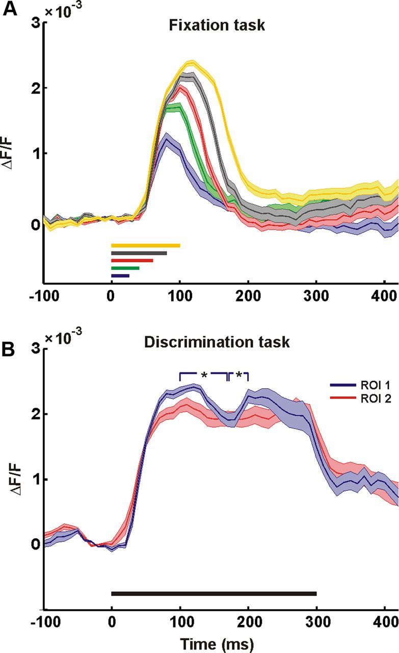
An off-response cannot explain the late neuronal modulation. A, Time course of responses evoked by a scramble stimulus with variable duration in a fixation task (i.e., a naive monkey was required to fixate without the report about the stimulus category), averaged over 227 pixels in the center of the chamber. Colors denote the stimulus duration time: blue, green, red, gray, and yellow correspond to 25, 40, 60, 80, and 100 ms, respectively. Line width denotes ±1 SEM over 15 trials. B, Time course of responses evoked by a 300 ms stimulus presentation in a face/scramble discrimination task, averaged over 172 and 181 pixels in two separate regions of interests (ROIs). Line width denotes ±1 SEM over five trials (carefully checked for eye movements); black bar, stimulus presentation. The blue ROI exhibits significant modulation (Wilcoxon rank-sum test between t = 100 and t = 170 ms poststimulus onset, p < 0.005 and between t = 170 and t = 200 ms poststimulus onset, p < 0.005).

MATLAB software (Ver. 2008b, The MathWorks) was used for statistical analyses and calculations. The basic VSDI analysis consisted of (1) defining region-of-interest (only pixels with fluorescence level ≥ 15% of maximal fluorescence were analyzed, (2) normalizing to background fluorescence, and (3) average blank subtraction (see more details and schematic illustration of the basic VSDI analysis in Ayzenshtat et al., 2010). For each recording session the VSDI signal was averaged over all the correct trials and the averaged signal used for further analysis (except for single-trial decoding and for error-trials analysis, see below).

Eye movements

Eye positions were monitored by a monocular infrared eye tracker (Dr. Bouis Devices), sampled at 1 kHz and recorded at 250 Hz. Only trials with tight fixation during stimulus presentation were chosen for further analysis. Typically, due to the brief stimulus presentation and to microscaccdic inhibition induced by the onset of stimulus presentation (Engbert, 2006; Rolfs et al., 2008; Meirovithz et al., 2012), we found almost no microsaccades during the first 200 ms poststimulus onset (the neuronal data analysis performed in this study was restricted to this time period). Therefore, the differences in the neural responses evoked by different stimuli cannot be explained by microsaccades.

Retinotopic mapping

Retinotopic mapping was obtained using optical imaging of intrinsic signals and VSDI. The retinotopic mapping of V1 using intrinsic signals has been described elsewhere (Shmuel et al., 2005). Briefly, to obtain retinotopic maps we conducted optical imaging of intrinsic signals (Fig. 2D) when the monkey was fixating and presented with high-contrast bars, horizontal (6 × 0.25°) and vertical (0.25 × 6°). As the imaging area lay near the V1/V2 border, horizontal bars in the visual field were mapped into bands in V1 that were approximately orthogonal to the V1/V2 border and vertical bars in the visual field mapped into bands approximately parallel to that border (Fig. 2D,E). The border between V1 and V2 was experimentally detected using ocular dominance maps. Complementary retinotopic mapping was obtained using VSDI when presenting small stimuli at variable eccentricities (single Gabors or individual face features, e.g., an eye) during a fixation paradigm.

Figure 2.

Analytical 2D mapping of the visual stimuli onto cortical space. A, An example of a stimulus as seen in the visual field, shown here against a polar grid. B, Enlargement of the stimulus zone in A. C, The stimulus zone in B after applying the analytical spatial transformation. D, Top, A series of intrinsic imaging activation patterns evoked by a vertical bar (0.25 × 6°) separately presented at different locations parallel to the LVM: LVM −0.5°, LVM −1.5°, VM −2.5° (−, to the left of LVM in the contralateral hemifield). Bottom, A series of activation patterns evoked by a horizontal bar (6 × 0.25°) separately presented parallel to the HM: HM −2.5°, HM −3.5° (−, below HM). Insets, Stimulus positions relative to the fixation point (red dot). E, Image of the blood vessel pattern in V1 taken on one VSDI experiment. The solid red lines mark the retinotopic mapping of the Cartesian lines shown in D. Dashed red lines, the borders between V1 and V2 and the LUS; black asterisks, two anchor points used for image registration; black dots, six points for optimizing the model's fit (see Materials and Methods; note, the intrinsic imaging recording and the VSDI recording were done on separate imaging days, therefore due to the relative angle between the camera and the cortical surface the blood vessels may seem slightly shifted between D and E). F, The spatially transformed stimulus (from C) after image registration on the exposed cortical surface. LUS, lunate sulcus; UVM, upper vertical meridian; LVM, lower vertical meridian; HM, horizontal meridian, A, anterior; P, posterior; M, medial; L, lateral.

2D analytical mapping of visual stimuli

To analytically map the visual stimulus into cortical coordinates we implemented the model proposed by Schira et al. (2007, 2010). The model suggests that the map of the visual space in V1, symbolized by the function w, is defined by the following:

where E is eccentricity, P is polar angle, k is a scaling constant, and a is a structural parameter. The input polar angle P is defined by the following:

where θ is the original polar angle, and α is a compression parameter reflecting the angular compression along the iso-eccentricity curves. f_a is a shear function defined by the following:

We examined both the monopole and the dipole versions of the model (Schira et al., 2007, 2010), and found the monopole version yielded a better fit to our experimental data than the dipole model. This was expected due to the close proximity of the exposed cortex to the fovea. This model includes three free parameters (k, a, α), requiring us to determine their optimal values in our imaged visual cortex. To do so, we first applied the spatial transformation using an initial set of parameters. Next, we used eight reference points for which both retinal and cortical coordinates were formerly and independently determined by optical imaging of intrinsic signals and VSDI (see above, Retinotopic mapping), to perform the following: (1) the transformed stimulus was registered (a linear transformation including only translation, rotation, and scaling) on the exposed cortical surface using two of the reference points as anchors and (b) we measured the root-mean-square deviation (RMSD) between the analytical coordinates and the empirical coordinates of the other six reference points. An optimal fit of the model was obtained by iterating through the parameter space (1 < k < 20), (0.2 < a < 4), and (0.3 < α < 1) to minimize the RMSD (Fig. 2E). The optimal representation of the source image on our monkeys' primary visual cortex was achieved with a = 0.57, k = 7.7, and α = 0.52 for monkey C, and a = 0.46, k = 4.87, and α = 0.51 for monkey L. Two of the model's free parameters (a, k) converged to optimal values similar to those previously reported in monkeys and humans (Schira et al., 2007, 2010). However, the global shear parameter (α) converged to ∼0.5 (previously reported α = 1), which may reflect the variability among animal species and/or unpredicted anatomical variations (see Discussion).

For further validation of the model's fit, we also applied the spatial transformation on a simpler stimulus (e.g., a Gabor array) and examined the correspondence between the neural response and the response expected from the analytical transformation (data not shown).

Computing the expected response for local attributes

RGB values of the stimulus were first converted into luminance values using a conversion function measured from our CRT monitor (using ColorCAL colorimeter; Cambridge Research Systems), which fitted an exponentiation with a power of 2.2 for the different RGB components. The luminance values were the sum of the three RGB components (Fig. 3A,B). Then, for each pixel in the image, the local luminance and local contrast were computed (Fig. 3C) according to Mante et al. (2005). Briefly, we used circular patches with diameter of 0.3° in which the local luminance of a patch was defined as follows:

where N is the total number of pixels in the patch, L_i is the luminance of the ith pixel, and w_i is the weight from a windowing function.

Figure 3.

Computing the expected neural response. Top, A, Example of a visual stimulus. B, The stimulus in A after conversion of each pixel from RGB to luminance values (maximum luminance of the screen = 75 cd × m⁻²). C, The local luminance (above) and local RMS-contrast (below) obtained by the weighted sum of a circular patch with a radius of 0.15°. D, The stimulus luminance and RMS-contrast shown in C, operated on by a nonlinear function (Naka–Rushton). E, The expected luminance response (above) and the expected contrast response (below) obtained by the weighted sum of a circular population RF (with size that varied linearly as a function of eccentricity). F, The expected luminance and contrast response after spatial transformation to cortical coordinates of V1 (Fig. 2; see Materials and Methods). Bottom, Model validation. Computing the expected neural response of a single Gabor stimulus. A, A Gabor element presented over a gray background. The red dot represents the fixation point of the monkey. B, The expected luminance and contrast response of a single Gabor, after spatial transformation to cortical coordinates (calculated as described above). C, The neural population response evoked in V1 by the presentation of a single Gabor, averaged over two time frames at 60–70 ms poststimulus onset (shown after 2D Gaussian filter with σ = 1.5 pixels). The spatial correlation values between the expected and the observed response are 0.58, 0.83 for the local luminance and local contrast, respectively, calculated over 452 pixels.

The local RMS-contrast of a patch was defined as follows:

The window weighting function was a circularly symmetric raised cosine as follows:

where d is the patch diameter; (x_i, y_i) is the location of the ith pixel in the patch; and (x_c, y_c) is the location of the center of the patch. The weights were normalized to sum to 1 as follows:

To calculate the local luminance and local contrast of pixels close to the edges of the image, we used the luminance value of the gray screen (37 cd × m⁻²) whenever parts of the patch fell outside the boundaries of the image.

The local luminance and local contrast were then operated on by the hyperbolic function (Naka–Rushton) as follows:

with q = 3 and L₅₀ = 0.1 (Sit et al., 2009; Meirovithz et al., 2010), to account for the nonlinearity response of V1 neurons to contrast and luminance (Fig. 3D). Next, we applied population RF. We averaged the local responses on circular weighted patches (again we used raised cosine weights). Since we recorded population response of neurons from eccentricities of 1–5°, whose RF size varied with eccentricity (Angelucci et al., 2002), we used patches with a diameter that varied linearly between 0.35 and 1.25° as a function of eccentricity (Fig. 3E). The last step (Fig. 3F) was to apply the spatial retinotopic transformation we described previously and in Figure 2. The resulted outcome of these steps was maps of the expected neural response for local luminance and contrast (Fig. 3F). Finally, we also tried to implement our model without applying Naka–Rushton function; however, in this case the fitting of the VSDI data to the model decreased significantly.

Spatial correlations

We calculated the Pearson correlation coefficient (r) between the expected response (x), either luminance or contrast (see above) and the neural response (y) for individual images according to the following:

where p is every pixel in V1. r was calculated on each time frame separately using N pixels (N varied between 2034 and 2515). r was calculated separately for faces and scrambled images (phase perturbation and segment scrambling; Fig. 4E,F, right).

Figure 4.

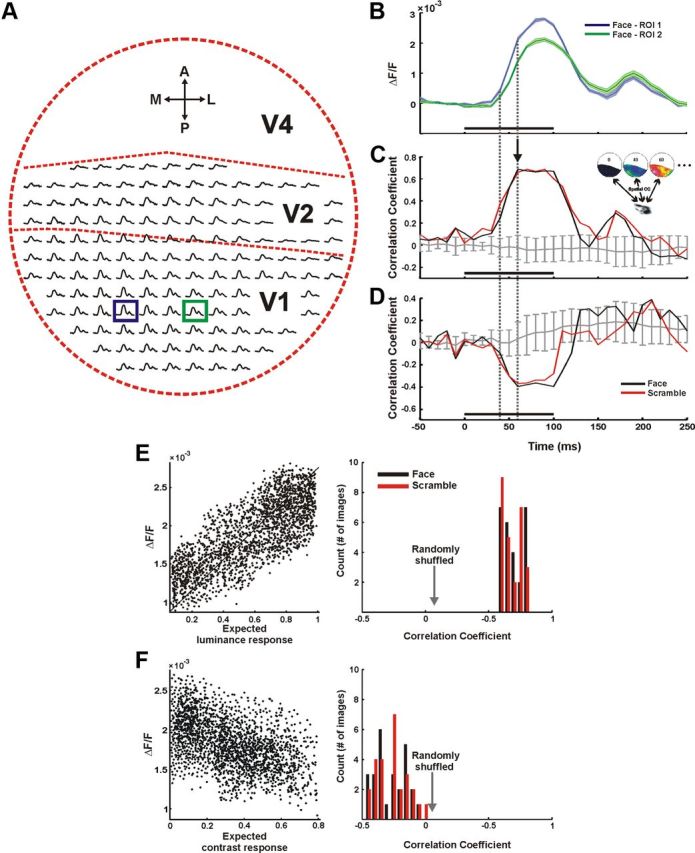
Spatial correlation between the maps of the population response and the expected response. A, Neural response time course along the imaged cortical space evoked by a face stimulus. Each plot corresponds to the mean signal averaged over 1 × 1 mm² (6 × 6 pixels). Dashed red lines schematically mark borders between cortical regions. B, Enlargement of the signals averaged over the region of interest (ROI) in the blue and green boxes in B. Trace width denotes ±1 SEM over 28 trials; the black bar represents the stimulus presentation time. C, D, Typical example of spatial correlation between the neural response (spread over 2034 pixels in V1) and cortical mapping of the expected luminance response (C) and the expected contrast response (D) as a function of time (see Materials and Methods). Black and red lines correspond to a coherent face stimulus (shown in A and B) and a scramble stimulus, respectively. Gray curve, correlation between the measured neural activity and the expected activity computed on a randomly shuffled set of stimuli (mean ± SD, n = 50). Dashed gray lines, the first time point exhibiting significant correlation and the time point with maximal correlation. Black bar denotes stimulus presentation. E, Left, Shows an example of a scatter plot of the expected luminance response of one face stimulus versus the neural response of all the pixels in V1 during one frame (t = 60 ms after stimulus onset, marked with an arrow in D, r = 0.69). Right, Shows the histogram of the spatial correlation values of all the images presented to both monkeys (n_face = 26, n_scramble = 26, scrambled images include both types of scrambling) at t = 60 ms after stimulus onset. No significant difference was found between the face and scramble. F, Same as in E, only for the correlation between the expected contrast response and the neural response (r = −0.39).

Partial correlation was calculated according to the following:

which measures the correlation between x and y, controlling for z.

We computed the partial correlation between (1) the expected luminance response and the measured neural response, controlling for the effect of the expected contrast response, and (2) the expected contrast response and the measured neural response, controlling for the effect of the expected luminance response.

Local luminance and contrast correlation in the stimulus

Local luminance and local RMS contrast were calculated for every pixel in the image as described above (Eqs. 4–7) using a circular patch with a diameter of 0.3°. Pearson correlation coefficient (r) was calculated according to Equation 9 between the local luminance and the local contrast of each image in the dataset, using all the pixels composing the image.

Single-trial decoding

Classification algorithm.

The data were randomly divided into a training set comprising 70% of trials (both face and scramble) and a test set that included the remaining 30%. We used a support vector machine (SVM) classifier with a linear kernel. Other statistical classifiers such as k-nearest neighbors (with k = 5 and Euclidean distance) performed similarly using the same features. For classification control, we trained the classifier with a randomized trial category.

Feature selection.

Single pixel amplitude at single time frames provided the input to the classifier. Since our data included ∼2000 pixels over V1, we needed to reduce the feature space dimensionality. To do so, we first rank ordered the pixels according to the mutual information (MI) between the neuronal signal and the stimulus category in the set of training trials (Ayzenshtat et al., 2010). We then selected pixels, starting with those exhibiting the highest MI and adding pixels with gradually decreasing MI.

Analysis of error trials

A discrimination error trial is defined as a trial in which the monkey was presented with a face stimulus, but reported scrambled or vice versa. Apart from the error, the behavioral parameters in these trials were similar to those in correct trials (e.g., fixation time until stimulus onset or eye movements until the GO signal).

We compared the cortical activity in correct and discrimination error trials where the animal was presented with the same stimulus. As the monkeys performed correctly in 80–85% of the trials, our sample of correct trials was much larger than that of error trials. Therefore, to equalize the amount of noise between the groups, we randomly chose the same number of correct trials as error trials and calculated the neural response (A in Eqs. 11 and 12), averaged over this group of correct trials (the typical number of error trials per session was 4–7 trials). A total of 10 imaging sessions from both monkeys were used for the discrimination error analysis (in each session we had at least four error trials in every condition, face or nonface).

We then calculated the Pearson correlation coefficient (r) between the activity of a single trial (A_i) and the averaged “correct” activity (Ā). This was done for each correct trial and each error trial for every pixel in V1 (p) and every time window (W). We used a sliding window of 80 ms, starting at 150 ms before stimulus onset and continuing until 250 ms after stimulus onset. r values were averaged separately over all the correct trials and over all the error trials. To avoid bias, we used exclusive subsets of correct trials—one for calculating the average correct signal, and the other for calculating the single trial correlations.

The distance between the histograms of the correct and the error trials' correlations, was measured in d′ for every time window, separately as follows:

Results

Two monkeys, trained on a face/scramble discrimination task, were presented in each trial with either a color-natural image of a monkey's face or a scrambled version of the same image (Fig. 1A; see Materials and Methods). Using VSDI, we measured population responses evoked in the striate cortex (V1) by the presentation of these images. The dye signal measures the sum of membrane potential changes of all neuronal elements in the imaged area (Grinvald et al., 1999). Data were obtained from 26 imaging sessions in two hemispheres of two adult monkeys. On each session a different pair of images was presented for a fixed time interval (varying between 80 and 100 ms across sessions).

Population response evoked by natural images

Using VSDI we directly measured the spatiotemporal activation pattern evoked by a brief presentation of natural images. The temporal activation profile showed two distinct phases. The first phase was an early and rapid increase, starting ∼40 ms after the stimulus onset, reflecting an increase in neural population activity. This was followed by a second late phase, starting ∼160 ms after the stimulus onset (Figs. 1, 4A,B). As shown in Figure 1C, the two temporal phases showed different spatial patterns of activation. The first appeared over most of the imaged area, generating a heterogeneous activation profile, whereas the second was spatially confined. We therefore set out to characterize the two phases and study their stimulus–response relationship in detail.

To do so, we first generated a map of the expected population response by (1) computing a continuous retinotopic representation of the stimulus on the cortex, using a 2D analytical transformation of visual space into cortical space and (2) computing the population encoding of local attributes of the stimulus, which was followed by the retinotopic transformation in (1). After obtaining the expected response, we could spatially correlate between the maps of the observed neural response and the expected one, for each time point along the time course of the VSDI signal (see below).

2D analytical mapping of visual stimuli

To analytically transform the visual stimuli into cortical coordinates we used a retinotopic model suggested by Schira et al. (2007, 2010). Analytical transformation of the stimulus was followed by image registration and an iterative optimization process, yielding an optimal representation of the source image on the primary visual cortex (Fig. 2; see Materials and Methods and Eqs. 1–3). Briefly, we applied a spatial transformation to each point of the stimulus in the visual field in a polar coordinate system (i.e., as a function of its polar angle and eccentricity; Fig. 2B,C). Next, we registered the transformed stimulus over the cortical surface using a set of retinotopic points (Fig. 2D–F). The cortical coordinates of these points were obtained in a separate set of imaging experiments using a small set of stimuli composed of bars and point stimuli (Fig. 2D,E; see Materials and Methods). Finally, we used a separate set of points to optimize the model's free parameters by aiming to minimize the RMSD between their measured cortical coordinates and their analytical cortical coordinates (see Materials and Methods). Since on each VSDI session the stimulus was positioned differently in the visual field, we could check the optimal fit of the model on each recording session and obtain a set of model parameters independent of stimulus location. The optimal fit yielded RMSD values of 0.35 ± 0.06 mm and 0.42 ± 0.10 mm for monkey C and monkey L, respectively (mean ± SD here and throughout). This means that the 2D accuracy of our mapping is up to ±2 pixels. A set of control experiments using a stimulus composed of an array of Gabor elements further validated the model's fit, showing a good fit between the measured neural activity and the 2D mapping of the Gabor array stimulus (data not shown).

Computing the map of the expected neural response based on local attributes

The main input of V1 is known to encode basic stimulus attributes (including local contrast and luminance). To compute the map of the expected neural response for local luminance and contrast in our stimuli we performed the following five steps (Fig. 3; see Materials and Methods). (1) Each pixel in the stimulus image was converted from RGB values to luminance values (Fig. 3A,B). (2) Next, we computed the local luminance and local RMS-contrast for each pixel in the image using a small circular patch that reflects the RF size of neurons in early visual stages (Fig. 3C; Eqs. 4–7) (Mante et al., 2005; Frazor and Geisler, 2006). (3) The resulting images were then operated on by a nonlinearity function (Naka–Rushton; Eq. 8), reflecting the nonlinear responses of neurons in V1 to luminance and contrast (Fig. 3D) (Albrecht and Hamilton, 1982; Shapley and Enroth-Cugell, 1984; Bonds, 1991; Heeger, 1992; Shapley and Lam, 1993; Carandini and Heeger, 1994; Geisler and Albrecht, 1997; Geisler et al., 2007). (4) Our next step was to apply the populations RF to take into account that the VSDI signal of each pixel in V1 reflects the membrane potential of neuronal populations (rather than single neurons), emphasizing subthreshold synaptic potentials (Grinvald and Hildesheim, 2004). Since the RF size depends on eccentricity, we used a patch size which varied linearly as a function of eccentricity (Angelucci et al., 2002, their “Summation Field”). As a result of these RF characteristics, the outcome images are somewhat blurred. Step 5 (Fig. 3F) was to apply the spatial retinotopic transformation as described in the previous section and in Figure 2. In summary, the outputs of our model are maps of the expected neural response based on the local contrast and local luminance of the stimulus (Fig. 3F).

Our simplified model is designed to estimate the expected neural response based on stimulus conversion to either local luminance or local contrast, followed by analytical retinotopic mapping. To validate the steps in our model, we used a stimulus composed of a Gabor element presented over a gray background. Indeed, Figure 3 (bottom) confirms that the model implementation reflects the local luminance and contrast of the original stimulus while subsequent steps show the expected neural response. We then calculated the spatial correlation between the map of the neural response and the map of the expected response and found that the neural response evoked by a Gabor stimulus was positively correlated with both the luminance and the contrast, where the contrast exhibits higher correlation (r = 0.58 and 0.83 for local luminance and local contrast, respectively).

Our model did not take into account other stimulus attributes known to be represented in V1, such as orientation, spatial frequency, or color. We were interested in imaging a large field of view, and therefore used a relatively large pixel size of 170 × 170 μm², which is approximately the size of an orientation, spatial frequency, or a color column in V1. Therefore, it is reasonable to assume that the response in each pixel is influenced by several orientations, color, and spatial frequency domains, which make it difficult to resolve their effects at the spatial domain, i.e., at the pixel level.

All of the above steps generated the expected neural response (to local attributes) that was spatially mapped onto the primary visual cortex in eccentricities of ∼1–5°. This enabled us to compute the spatial correlation with the measured population response evoked in thousands of points spread over V1.

Spatial correlation between the maps of the expected response and the early measured response

We calculated the spatial correlation (Pearson correlation coefficient, r; Eq. 9) between the map of the expected response (Fig. 3F) and the map of the measured response, using all the pixels in V1 (Fig. 1C), on each time frame separately (Fig. 4C, inset). As we have shown above (Fig. 1), the VSDI signal clearly exhibits two temporally distinct phases of activity (Fig. 4A,B). Here, we will first focus on the early phase.

Local luminance

The expected luminance response showed a significant, high positive correlation with the neural response (Fig. 4C). This correlation started at ∼40 ms, (when the VSDI signal started to rise above baseline; Fig. 4B) and reached a maximal value of 0.69 ± 0.08 at 60 ms after stimulus onset (n = 52 images, data from both monkeys; Fig. 4E). This maximal value was sustained until 100 ms after stimulus onset without significant further modulation, declining shortly after the visual stimulus was turned off. Considering the sample size used to compute this spatial correlation (1800–2500 pixels in V1), a value of ∼0.7 is very high, meaning that almost 50% of the neural response variance during a single time frame could be explained solely by the local luminance of the stimulus (Fig. 4E). The remaining variance may be explained by other local attributes, which our model did not consider (orientation, spatial frequency, or color). There was no significant difference between the spatial correlations of face and scramble trials (0.69 ± 0.08 and 0.68 ± 0.07 at 60 ms after stimulus onset, respectively), further suggesting that during this early time, the information conveyed is mainly of the local luminance rather than perceptual effects. After the stimulus was turned off and the correlation declined to baseline, a second small rise in the correlation was shown during later times (along with the second modulation of the signal; Fig. 4B,C); however, further analysis revealed this correlation is not significant across sessions (see below, The relation between the stimulus content and the late neural response).

Local contrast

The spatial correlation of the expected RMS-contrast response showed a significant negative correlation to the measured neural response (−0.27 ± 0.13, face trials; −0.25 ± 0.13, scramble trials; Fig. 4D,F) during the early response phase, followed by a baseline value during the late phase.

However, the definition of contrast in a complex image is not straightforward (Peli, 1990). Basically, it is the local luminance modulation divided by the local mean luminance at each point of the image. The local RMS-contrast is unsigned and normalized by the mean local luminance (Fig. 3C; see Materials and Methods). As a result, a local patch with low mean luminance (i.e., consists of mostly dark pixels) and very few bright pixels, will yield high contrast whereas a local patch with high mean luminance (i.e., consists of mostly bright pixels) and very few dark pixels, will yield low contrast.

To independently test the correlation of the neural response to the local luminance and the local contrast of the stimuli, we needed to examine the contrast–luminance relationship of our stimuli. As shown in previous study (Lindgren et al., 2008), we also found a spatial dependency between the local luminance and contrast of our stimuli, specifically a significant negative correlation (−0.45 ± 0.13; averaged over 52 images with no significant difference between the face and the scramble images) (Fig. 3; see Materials and Methods). We therefore computed the partial correlation (i.e., the correlation between two variables after excluding the external effect of a third; Eq. 10) between the expected luminance response and the measured neural response, controlling for the effect of the expected contrast response and vice versa (see Materials and Methods). The partial correlation values to the expected luminance response were almost unchanged (0.71 ± 0.14), whereas the partial correlation to the expected contrast response were closer to zero (−0.11 ± 0.18, averaged over the face and the scramble trials with no significant difference between them). That means that the neural signal carries information mainly about the local luminance of the stimulus independent of the local contrast, whereas the contrast information is largely dependent on the luminance.

Finally, we also computed an alternative model that accounts for local luminance adaptation in the retina. This was implemented by applying the nonlinearity (Naka–Rushton function) using a variable L₅₀ that was computed separately for each pixel. The local L₅₀ for each pixel was defined as the mean local luminance in a circular patch of 0.5° (i.e., the luminance gain for each pixel varied locally). The resulting expected neural response reflects the local signed contrast (data not shown). We note that in this model the expected neural response is very similar to the expected luminance response (Fig. 3F), therefore we obtained a significant positive correlation as in the model we have shown in Figure 3, yet their values were smaller (r = 0.52 ± 0.13).

In summary, we found that the early response phase encodes information about the low-level, local attributes of natural stimuli.

Single-trial discrimination

To study how much information the neural activity conveys about the stimulus category at different times, we tested whether we could use the neural activity to discriminate between face and scramble stimulus categories on a single-trial level. A binary classifier (see Materials and Methods) was trained to decide whether a trial was a face or a scramble trial. A random subset with 70% of the trials was used for training and the remaining 30% for testing. The classifier performance at each time frame was assessed as a function of the number of pixels (Fig. 5A). Using, for example, 93.2 ± 42.2 pixels gave a classification performance level of 94.4 ± 3.8% in the early time frame (50 ms after stimulus onset, averaged across imaging sessions from both monkeys, chance = 50%). In the late time frame (160 after stimulus onset) maximal classification reached a lower value of 81.6 ± 4.7% using 120.2 ± 41.1 pixels.

Figure 5.

Single-trial readout performance. A, Performance of an SVM classifier (see Materials and Methods) at the single trial level as a function of the number of pixels used (example of one imaging session, n = 56 trials, 28 face trials, 28 segment scrambling nonface trials). Blue and red traces, Classification performance using neural activity at t = 50 ms and t = 160 ms after stimulus onset, respectively (mean ± SEM, n = 50 iterations, face vs phase perturbation nonface). Gray trace, Performance of the classifier trained with the randomized trial category (control). B, Maximal performance of the classifier over time (using 125 pixels), showing two phases of information processing. Blue and red arrows mark the time frames plotted in A.

To summarize, maximal performance of the classifier demonstrated two phases of information processing, corresponding to the two response phases. The first was during the early processing of the stimulus yielding high-classification performance (Fig. 5B). This was not surprising, considering the differences among the low-level features of the face versus scramble stimuli that are expected to be encoded in the early input of V1. However, the significant performance of the classifier during the late phase suggests that V1 still holds some information about the stimulus category, even when the stimulus is no longer present in the visual field and after the early response has returned to baseline. Thus, we further asked what information is conveyed in the late phase and how it differs from the early stimulus-locked activity.

The relation between the stimulus content and the late neural response

As shown in Figure 4B, the second response phase consisted of an increase in activation starting ∼160 ms after stimulus onset. Unlike the first phase, the spatial correlation between the response in this late phase and the local attributes of the stimulus was found to be not significant (both with the luminance and with the contrast, r = 0.10 ± 0.13, 0.07 ± 0.16, respectively, averaged over all the face and scramble stimuli, calculated as described above).

To further investigate the activity in the late response, we asked whether it is mainly an off-response, reflecting the stimulus offset. Hence, we presented our stimulus to a naive monkey during a passive fixation task (i.e., a third monkey that was not trained on a face/nonface discrimination task). The monkey was not required to report the content of the image, but only to maintain fixation. We found that when the monkey was not required to attend and report the image category, the late phase did not occur (Fig. 6A). Furthermore, to study whether the late modulation persisted during stimulus presentation (in a discrimination task), we used a longer presentation of the stimulus and extended the stimulus duration to 300 ms. We found a significant late modulation occurring at times similar to those observed with the briefer stimuli, while the stimulus remained present in the visual field for 300 ms (Fig. 6B). We note that the late modulation was much smaller for the long stimulus duration compared with the brief stimulation. However, this might be expected, as during the long stimulus presentation, the retinal input keeps on streaming into V1 and thus “diluting” the modulation of the late phase. Altogether, these findings suggest that the late response does not reflect merely an off-response. In fact, the late response was previously reported to occur at similar or partially overlapping time windows (Lamme, 1995; Zipser et al., 1996; Supèr et al., 2001a,b), and has been linked to higher visual functions such as pop-out, grouping, figure-ground segregation, working memory, and spotlight of attention. Here we further show that this late phase occurred during natural images processing. Since we measured the neural activity from a large cortical area, we could study the late response in both time and space with respect to higher aspects of visual processing.

When we examined the characteristics of the late phase, we noticed it was less time locked to the stimulus presentation compared with the early response, and more localized in the spatial domain. an increase in the spatial variance across the responses of V1 pixels. We therefore computed the spatial variance, i.e., the variance of the response amplitude across all the pixels in V1 (Fig. 7B; see Materials and Methods), for each time frame. This enabled us to identify the time frame potentially conveying essential information during the late phase (the time frame with the maximal spatial variance). The example in Figure 7A, B shows a late increase in the response variance peaking at ∼170 ms after stimulus onset which was not accompanied by a notable increase in the mean response amplitude (as opposed to the increase in the mean response seen in the early phase; Fig. 7A). This variance modulation indicated a potential increase in the information conveyed by the signal. We therefore calculated the distribution of the response amplitude at this time point of local maximum in the spatial variance. We found a bimodal distribution (Fig. 7C) that was consistent across all the imaging sessions. The bimodal distribution demonstrated a group of pixels that underwent an increase in amplitude, meaning a second neural modulation, and a larger group of pixels that remained approximately at baseline level of activity. This bimodality was not present during the early response, when activity was spread over most of the imaged area (Fig. 7A). To spatially characterize these groups, we mapped all the pixels in V1, assigning black and red color to each pixel based on its group (using a threshold set at the local minimum of the bimodal distribution). We observed a clear spatial separation between pixels belonging to the high-amplitude group and to the low-amplitude group (Fig. 7D). Although this threshold-crossing mapping resulted in some information reduction, it simplified the data and revealed an important spatial relation to the stimuli, as shown below.

Figure 7.

Spatial mapping of the late response. A, Example of VSDI amplitude distribution across V1 pixels as a function of time (one face stimulus imaging session, averaged over 30 trials, n = 2510 pixels, bin width = 10 ms). Color bar denotes normalized distribution; black bar denotes stimulus presentation time. B, The variance of the VSDI response across all V1 pixels, i.e., the spatial variance, as a function of time. C, Bimodal distribution in VSDI amplitude at time marked with arrow in B (t = 170 ms after stimulus onset). Dashed gray line marks the amplitude threshold for the mapping in D. Inset shows a unimodal amplitude distribution at t = 60 ms after stimulus onset. D, Neural activity map in V1 at t = 170 ms after stimulus onset. Black and red pixels are those below and above amplitude threshold, respectively. E, Distributions of distance-to-centroid of the black and red pixel groups in D.

Next we examined how this spatial distribution was related to the original stimulus and found that in face trials, pixels with high amplitude (Fig. 8, red) corresponded mainly to the center of the face whereas pixels with low amplitude (Fig. 8, black) corresponded to other parts of the stimulus (e.g., fur, image background). When the location of the face's center was shifted along the cortical space, the pixels exhibiting high amplitude were shifted along with it (Fig. 8i,iii). In scramble trials the same mapping (using the threshold defined in the face trials) produced sparser and more distributed activity over the cortical area (for both types of scrambling). To quantify the difference between the spatial activity patterns in the face and the scramble trials, we first calculated the centroids of the low- and the high-amplitude groups, defined as the mean spatial location of each group. We then calculated the distribution of the distances from the centroid of each pixel in the two groups. Computing the distance between these distributions (d′) allowed a quantitative comparison between them (Fig. 7E). The face trials showed a highly significant difference between groups (d′ = 1.55 ± 0.38; averaged over 18 imaging sessions from both monkeys), indicating that the late neural response was efficiently clustered in space. The spatial difference between the groups was significantly lower in the scramble images (d′ = 0.52 ± 0.17; both types of scrambling), implying that although there were two groups exhibiting significant amplitude difference, these groups were less localized in space. One explanation for this effect can be the spatial scrambling of image segments in the scrambled stimuli, which may lead to a less localized spatial activity. However, the low correlation of the late phase to the local stimulus attributes does not support this hypothesis.

Figure 8.

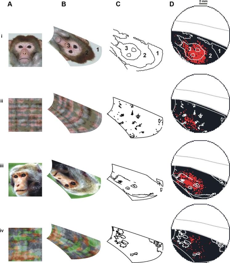
Linking the late neural response with stimulus features. Four stimuli superimposed over the map of V1 activity. A, Stimuli. B, Stimuli after spatial transformation. C, Contour line of the stimuli after spatial transformation (defined using a standard algorithm for edge detection for presentation purpose only). D, Contour line of the stimuli superimposed on the late response mapping after threshold crossing (as shown in Fig. 7; on each row the neural activity was averaged over 30 trials). 1, Area with maximal luminance of the image but located outside the face region. 2, Area with low luminance. 3, Area with high luminance inside the face region. Stimuli (i) and (ii) were positioned at x = 1.9°, y = 3.7° from the fovea (center of image), stimuli (iii) and (iv) at x = 1.8°, y = 3.7° from the fovea.

The 2D mapping of the stimulus onto the cortex can further demonstrate that the late phase is not directly related to the local luminance of the stimulus. As shown in Figure 8, we examined distinct regions with high and low local luminance along the mapping of the stimulus on the cortex, and compared them to the spatial pattern of the late neural response. In all the coherent face stimuli, there are regions of high luminance (which exhibit high amplitude during the early response) that did not exhibit a late neural response (Fig. 8, region #1), while other regions of high luminance did exhibit a late neural response (Fig. 8, region #3). Therefore, these results further support the notion that the late modulation was not merely a late reflection of the luminance.

Altogether, these findings suggest that the late response does not have a strong relation to the stimulus local attributes, and a possible explanation for the less localized activity in the scramble stimuli during the late phase may be the lack of a well defined context and/or coherent percept (see Discussion). In fact, a reasonable hypothesis would be that the late phase includes aspects of higher visual processes, such as perceptual processing of the stimulus. The analyses we present below strongly substantiate this suggestion.

Neural correlates of behavior

To test whether the late neural response carried information on the global percept of the visual stimulus, we correlated the neural response with the animal's behavior. To do so, we examined the animal task performance using analysis of discrimination error trials.

We performed our analysis on correct trials versus discrimination error trials, i.e., trials in which the animal was presented with a face stimulus, but reported scramble and vice versa: trials in which the animal was presented with a scramble stimulus, but reported face. This means, that in both correct and error trials the animal was seeing exactly the same stimulus; however, its behavioral report was different. Comparing correct and discrimination error trials could reveal whether the behavioral difference was reflected in the imaged V1 activity (Fig. 9, an example from one recording session). To do so, for every pixel in V1, we calculated the temporal correlation coefficient (r) between its activity in a single trial and its average “correct” activity (see Materials and Methods). This was done separately for correct and error trials using a sliding time window (Eqs. 11 and 12). Figure 9A–C shows the r value distribution of the correct and error trials, for all the pixels in V1 before the onset of the stimulus, during the early response and during the late response. We then computed the distance (d′) between the correct and the error trial distributions as a function of time (Eq. 13). The d′ of the early response phase was very close to zero, 0.005 ± 0.020, when averaged over 10 imaging sessions from both monkeys. However, during the late response phase the difference between the correct and error distributions was much larger and significant (Fig. 9C). The d′ value reached a maximum during the late phase in both face trials and scramble trials (Fig. 9D,F). When averaged over 10 imaging sessions from both monkeys, the d′ in the late phase reached a value of 0.998 ± 0.134. There was no significant difference between the d′ of face and scramble trials (neither in their values nor in their dynamics). Altogether, these results show that the response dynamics of error trials was similar to those of correct trials during the early phase (not surprising considering that both correct and error trials share the same visual stimulus) but deviated significantly from the “correct activity” during the late phase, before the animal reported on the perceived stimulus.

Figure 9.

Error trials analysis. A–C, Distribution of the temporal correlation coefficient, r, (see Materials and Methods) in face stimulus trials, averaged over the correct trials (blue, n = 7) and the error trials (red, n = 7) in one recording session. For adequate comparison, we matched the number of correct and error trials. The distributions are shown before stimulus onset (A), during the early response (B), and during the late response (C). Temporal correlations were calculated in a window of 80 ms. D, Distance between the correct and the error histograms (d′) as a function of time. Note the time scale denotes the center of the time window used to calculate the temporal correlations. Arrows, Time points corresponding to the distributions in A–C. E, Map of all the pixels in V1 with r value above (gray pixels) and below threshold (black pixels). Threshold is marked by the dashed gray line in C. Left and right show the correct and the error trials, respectively. F, G, As in D and E, only for scramble stimulus trials (segment scrambling; n = 7 correct trials and 7 error trials). The data here were obtained from a single recording session.

Having discovered when this effect occurs, we next examined where it occurs. A threshold was set on the above correlation value (the 75% percentile of the distribution of correct trials; Fig. 9C). Using this threshold we created two maps for face trials, where V1 pixels with r value above the threshold were marked with gray and V1 pixels with r value below the threshold were marked with black. One map was generated for the correct trials and another map was generated for the error trials. The map of the correct trial correlations showed a compact cluster of pixels, while the map of the error trial correlations was much sparser (Fig. 9E). For the scramble stimulus trials, the opposite occurred: the map of the correct trial correlations showed a wide spatial distribution, whereas the map for the error trials (i.e., the monkey saw a scrambled image but reported face) correlations showed a clustered and more spatially compact set of pixels (Fig. 9G; see quantification below). Serendipitously, we found that the cluster of pixels reflecting the high correlations of correct face trials corresponds well with pixels located at the center of the face (Fig. 9E, contour line, left).

These results suggest that on trials where the monkey reported seeing a face (whether these were error or correct trials), pixels that were highly correlated with the correct activity appeared in a clustered area (see analysis in the next paragraph). In the correct trials, this cluster corresponded to the central parts of the mapped face. Similar results were obtained from five recording sessions in which both monkeys made a significant number of discrimination errors for both the face and the scramble condition.

To quantify the difference in spatial activity between correct and error trials, we calculated the centroid of the group of pixels above threshold and the mean distance of each pixel from the centroid. In face trials this distance exhibits significant difference and was 2.14 ± 0.46 and 3.82 ± 0.95 mm in correct and error trials, respectively (Wilcoxon rank-sum test, p < 0.005). In scramble trials (both types of scrambling), it was also significantly different and was 3.61 ± 0.7 and 2.39 ± 0.43 mm in correct and error trials, respectively (Wilcoxon rank-sum test, p < 0.005). Thus, the neural response in V1 is correlated with the animal's perceptual report, suggesting that V1 may receive late neural input related to the perceived content of the stimulus. Finally, we validated that the above correlation patterns were not due to differences in response amplitude between correct and error trials. We further elaborate on the relation between the spatial correlation patterns and the animal's perceptual report (see Discussion).

Another behavioral aspect we studied was the animal's reaction times (RT). However, we did not find a significant correlation between the neural activity and RT (data not shown).

Finally, we note that due to the brief stimulus duration as well as microscaccdic inhibition induced by the onset of stimulus presentation (Engbert, 2006; Rolfs et al., 2008; Meirovithz et al., 2012) we found almost no microsaccades during the first 200 ms poststimulus onset (the neuronal data analysis performed in this study was restricted to this time period). Therefore, the differences in the neural responses evoked by different stimuli cannot be explained by microsaccades (see Materials and Methods).

Discussion

Population activity was measured simultaneously from thousands of points in V1 using VSDI, while the monkey performed a visual discrimination task. Analytical 2D mapping of the stimulus into cortical coordinates enabled us to demonstrate a robust relation of the early neural response to local stimulus attributes and a later response correlating with the animal's perceptual report.

Analytical mapping of the visual stimulus into cortical space and computation of the expected neural response

Few models have been proposed to account for the mapping of the visual space onto V1 (Schwartz, 1977; Polimeni et al., 2006; Schira et al., 2007, 2010). We used a recent model suggested by Schira et al. (2007, 2010) and found a good fit to our data as evident from the small RMSD values and a good fit to a Gabor array stimulus (data not shown). We also found that the α parameter (the angular compression along the iso-eccentricity curves) converged here to a smaller value than previously reported, suggesting a greater elongation of the V1 cortical surface in one dimension, parallel to the VM. This means that we found a greater anisotropy in the visuotopic map of V1 in M. fascicularis. Distortions of the V1 visuotopic map (Das and Gilbert, 1997) or curvatures of the cortical surface during imaging may also affect the fit to the analytical model. For example, the cortical surface can appear more concave or convex in our dataset depending on (1) the difference between the intracranial pressure and the fluid pressure above the artificial dura, (2) the position of the artificial dura, and (3) the angle between the camera lens and the cortical surface.

To calculate the expected neural response we applied the nonlinear Naka–Rushton function, previously used to describe the luminance-response function of retinal neurons (Naka and Rushton, 1966; Baylor and Fuortes, 1970; Boynton and Whitten, 1970) and the contrast-response function of V1 neurons (Albrecht and Hamilton, 1982; Li and Creutzfeldt, 1984; Sclar et al., 1990; Geisler and Albrecht, 1997; Tolhurst and Heeger, 1997). To obtain an expected neural response, we used the Naka–Rushton function with a fixed set of parameters across the entire visual stimulus and the entire image set (except in the case of the local luminance adaptation model). Despite this nonoptimal estimation we still obtained highly significant positive correlations with the stimulus luminance (Fig. 4E).

Neural correlates of local luminance and local contrast and the relation between luminance and contrast in our set of images

The VSDI signal showed a strong positive correlation to the expected local luminance response, mainly in the first response phase. The high correlation value, ∼0.7, suggests that the local luminance of natural images accounts for ∼50% of the neuronal variance in V1 shortly after stimulus presentation (∼60 ms poststimulus onset). This finding is in agreement with recent studies showing that there are surface-responsive neurons that convey information about luminance. For example, Roe et al. (2005) found that around 50% of the sampled V1 neurons were significantly modulated by local-luminance changes. Geisler et al. (2007) also showed that most of the neurons in the primary visual cortex carry substantial local luminance information, although we note that our local luminance changes are much smaller than the ones reported in this study. Vladusich et al. (2006) also concluded that luminance processing predominates over contrast integration in the vast majority of surface-responsive neurons in V1, and Tucker and Fitzpatrick (2006) showed that layer 2/3 neurons of tree shrews' primary visual cortex, are sensitive to large-scale changes in luminance.

The local RMS contrast was negatively correlated with the population response evoked by our set of natural images (unlike the case of the Gabor stimulus) (Fig. 3, bottom; Meirovithz et al., 2010). However, this can be linked to the fact that in our set of natural images we found a significant negative spatial correlation between the local luminance and contrast. Indeed, a recent work (Lindgren et al., 2008) has shown that there are spatial dependencies between the local luminance and contrast of natural images. This is different from earlier studies that have shown that natural images exhibit a weak negative correlation between local luminance and local contrast, implying the two are nearly statistically independent (Mante et al., 2005; Frazor and Geisler, 2006). This discrepancy may result from our unique stimulus set (coherent and scrambled faces), which comprises of only two stimulus categories with a maximal luminance of 75 cd × m⁻², while previous studies used a large set of scenery images exhibiting a wide range of luminance values (∼50–5000 cd × m⁻²).

To correct for the local luminance–contrast relation we computed a partial correlation and found no significant correlation between the local RMS contrast and the population response. This is surprising, mainly due to many previous studies demonstrating contrast coding in V1 (Albrecht et al., 2004), including when dealing with natural images (Weliky et al., 2003). A possible explanation could be related to the way we correlated the observed response with the expected one. Here, we investigated the population responses measured from a continuous space in V1 that corresponds to a continuous space in the visual field. We then computed a spatial correlation between two maps composed of thousands of points at single time frames. We did not integrate the neural response over time, nor did we subsample the cortical space. Hence we were able to see the neural correlates to the whole image, and not only to few isolated patches within the image, as was done in previous studies.

Another possible explanation might be related to the contrast distribution within the stimuli that is much more diverse and widespread in natural images than in simple artificial stimuli (Fig. 3). The presence of contrast outside the classical RF has been shown to have a suppressive effect, which is contrast dependent (Levitt and Lund, 1997; Jones et al., 2001; MacEvoy et al., 2008). It is possible therefore, that a diverse contrast distribution will induce widespread suppression on the neuronal activity, which would result in a lower overall contrast response.

Population activity in the late neural response phase and behavioral correlates

The late neural modulation in V1 response (∼100–300 ms after stimulus onset) showed nonsignificant correlation to both local luminance and contrast. It occurred during longer stimulus presentations (300 ms), and was absent from the activity of a naive fixating animal that was not required to discriminate. These two findings suggest that the late phase cannot be explained by an off-response effect. Previous studies have suggested that the late modulation reflects aspects of higher level visual processing, such as figure-ground segregation (Lamme, 1995; Zipser et al., 1996; Supèr et al., 2001b), working memory (Supèr et al., 2001a), and attention (Pooresmaeili et al., 2010). The short stimulus presentation enabled us to study this response after stimulus offset, i.e., in the absence of direct retinal input. The occurrence of the late response after stimulus offset further supports the hypothesis that it may result from top-down processing (Lamme et al., 1998; Roland et al., 2006).

It can be argued that the late phase of activity is directly related to the motor planning and execution of the reporting saccade (which was absent during the fixation task). However, Supèr et al. (2001b) have shown that late activity in macaque V1 preceding a reporting saccade is not directly associated with the subsequent motor response. Furthermore, Supèr and Lamme (2007) have found no relation between the amplitude of the late V1 activity and the reaction time of visually guided saccades (as opposed to memory-guided saccades) in a figure-ground detection task. This is in accordance with our results, where we found no correlation between the late phase characteristics and the animal reaction time of the reporting saccade. Finally, even for memory-guided saccades, Supèr and Lamme (2007) report that V1 activity associated with a subsequent saccade is spatially specific and found uniquely at the area corresponding to the target location of the saccade. The visually guided saccades in our paradigm were directed to targets located at peripheral eccentricities (>7°), which is outside our imaging area.

Our single trial analysis unexpectedly revealed that during this late phase there was still substantial information on stimulus category—responses to face or scramble were significantly distinguishable. Analysis of discrimination error trials demonstrated that the late phase correlated with the animal's behavior (whereas the early phase did not carry any information on the discrimination errors) and revealed regions relevant to the animal's discrimination performance. We note that although the late phase correlates with the animal discrimination errors, this does not necessarily mean that it should hold more information regarding the stimulus category than the early phase (as demonstrated by the higher classification performance during the early phase). In fact a reasonable assumption is that the first phase will carry maximal information on the stimulus content (local features of the coherent face or local features of the nonface), which is directly related also to the stimulus category (face or nonface). We suggest that based on the information carried in the first phase, the monkey performs a perceptual decision that is reflected in the second phase and therefore correlates with the animal's behavior.

Late neural activity may convey higher aspects of stimulus processing

The late neural activity appeared in regions corresponding to the center of the face (Figs. 7–9). What might be a possible interpretation for this? The face/scramble discrimination task required the monkey to make a perceptual analysis of the stimulus. We neither instructed nor provided any information regarding figure-ground segregation nor did we control the animal's spatial attention. The monkey could use any strategy in segmenting and categorizing the image and was free in his attentional focus. We assumed that, when the monkey was presented with a coherent face stimulus, the center of the face (which is highly informative for these social animals) would automatically attract visual attention, while the scrambled images contained no consistent salient spatial feature drawing the attentional spotlight (Fig. 8). The appearance of the late response in trials with scrambled images lacking a coherent percept may therefore reflect spatial wandering/anchoring of the animal's attention to various points of interest in the nonsense images. As would be expected in this case, the response in scramble trials showed a more distributed spatial organization and increased spatial variability over trials without significant change in amplitude. It is also less likely that the late response resulted from figure-ground segmentation, as there is no well defined figure or ground in the scrambled images.

The error trials analysis also supports the spatial attention of the animal. As seen in the correlations spatial patterns,trials in which the animals reported perceiving a face (i.e., correct face trials or error scrambled trials) showed a more spatially compact pattern suggesting that the animal may extract the information from a relatively compact part of the stimulus: either the central part of the face that is comprised of a few informative features or from a small segment such as part of the eye/nose in the scrambled image. This may generate a compact neuronal representation in space, leading to a compact pattern of correlation. However, trials in which the animal reported perceiving a scrambled image (i.e., correct scramble trials or error face trials) showed a more spatially distributed pattern, suggesting that the animal had to use a wider examination of the image space. The animal may need to confirm that the scrambled segments are not linked in a manner that can generate a coherent face. This entails a wider wandering of the animal's attention to spatially distributed parts of the images and may lead to a wider neuronal representation in space, leading to a more distributed pattern of correlation.

These results support our previous analysis of the perceptual information conveyed during the late neural response in V1, in which we found that a coherent image is more compactly represented and hence efficiently characterized by fewer spatiotemporal patterns than a scrambled image (Ayzenshtat et al., 2010). Reduced activity in response to coherent stimuli in V1 has been found previously in humans (Murray et al., 2002) and is supported by theoretical models of predictive coding (Mumford, 1992; Rao and Ballard, 1999). The latter suggest that higher areas carry predictions of the bottom-up, stimulus-evoked neural activity based on previous knowledge while lower areas carry back the residuals, i.e., the error between the prediction and the actual activity. Such processing would lead to reduced activity when a “match” between the sensory information and the prediction is good and could consequently facilitate higher sensitivity to novel elements or stimuli.

Since the results of this study are based mainly on two behaving monkeys, future investigations are required to further establish the suggested function and characteristics of the early and late neural modulations existing within V1.

Notes

Supplemental Figures 1–9 for this article are available at http://neuroimag.ls.biu.ac.il/supplementary.html. This material has not been peer reviewed.

References

- Albrecht DG, Hamilton DB. Striate cortex of monkey and cat: contrast response function. J Neurophysiol. 1982;48:217–237. doi: 10.1152/jn.1982.48.1.217. [DOI] [PubMed] [Google Scholar]
- Albrecht DG, Geisler WS, Crane AM. Nonlinear properties of visual cortex neurons: temporal dynamics, stimulus, selectivity, neural performance. In: Chalupa LM, Werner JS, editors. The visual neurosciences. Cambridge: MIT; 2004. pp. 747–764. [Google Scholar]
- Angelucci A, Levitt JB, Walton EJ, Hupe JM, Bullier J, Lund JS. Circuits for local and global signal integration in primary visual cortex. J Neurosci. 2002;22:8633–8646. doi: 10.1523/JNEUROSCI.22-19-08633.2002. [DOI] [PMC free article] [PubMed] [Google Scholar]
- Arieli A, Grinvald A, Slovin H. Dural substitute for long-term imaging of cortical activity in behaving monkeys and its clinical implications. J Neurosci Methods. 2002;114:119–133. doi: 10.1016/s0165-0270(01)00507-6. [DOI] [PubMed] [Google Scholar]
- Ayzenshtat I, Meirovithz E, Edelman H, Werner-Reiss U, Bienenstock E, Abeles M, Slovin H. Precise spatiotemporal patterns among visual cortical areas and their relation to visual stimulus processing. J Neurosci. 2010;30:11232–11245. doi: 10.1523/JNEUROSCI.5177-09.2010. [DOI] [PMC free article] [PubMed] [Google Scholar]
- Baylor DA, Fuortes MG. Electrical responses of single cones in the retina of the turtle. J Physiol. 1970;207:77–92. doi: 10.1113/jphysiol.1970.sp009049. [DOI] [PMC free article] [PubMed] [Google Scholar]
- Bonds AB. Temporal dynamics of contrast gain in single cells of the cat striate cortex. Vis Neurosci. 1991;6:239–255. doi: 10.1017/s0952523800006258. [DOI] [PubMed] [Google Scholar]
- Boynton RM, Whitten DN. Visual adaptation in monkey cones: recordings of late receptor potentials. Science. 1970;170:1423–1426. doi: 10.1126/science.170.3965.1423. [DOI] [PubMed] [Google Scholar]
- Carandini M, Heeger DJ. Summation and division by neurons in primate visual cortex. Science. 1994;264:1333–1336. doi: 10.1126/science.8191289. [DOI] [PubMed] [Google Scholar]
- Das A, Gilbert CD. Distortions of visuotopic map match orientation singularities in primary visual cortex. Nature. 1997;387:594–598. doi: 10.1038/42461. [DOI] [PubMed] [Google Scholar]
- David SV, Vinje WE, Gallant JL. Natural stimulus statistics alter the receptive field structure of v1 neurons. J Neurosci. 2004;24:6991–7006. doi: 10.1523/JNEUROSCI.1422-04.2004. [DOI] [PMC free article] [PubMed] [Google Scholar]
- Engbert R. Microsaccades: a microcosm for research on oculomotor control, attention, and visual perception. Prog Brain Res. 2006;154:177–192. doi: 10.1016/S0079-6123(06)54009-9. [DOI] [PubMed] [Google Scholar]
- Felsen G, Touryan J, Dan Y. Contextual modulation of orientation tuning contributes to efficient processing of natural stimuli. Network. 2005a;16:139–149. doi: 10.1080/09548980500463347. [DOI] [PubMed] [Google Scholar]
- Felsen G, Touryan J, Han F, Dan Y. Cortical sensitivity to visual features in natural scenes. PLoS Biol. 2005b;3:e342. doi: 10.1371/journal.pbio.0030342. [DOI] [PMC free article] [PubMed] [Google Scholar]
- Field DJ. What is the goal of sensory coding. Neural Comp. 1994;6:559–601. [Google Scholar]
- Frazor RA, Geisler WS. Local luminance and contrast in natural images. Vision Res. 2006;46:1585–1598. doi: 10.1016/j.visres.2005.06.038. [DOI] [PubMed] [Google Scholar]
- Geisler WS, Albrecht DG. Visual cortex neurons in monkeys and cats: detection, discrimination, and identification. Vis Neurosci. 1997;14:897–919. doi: 10.1017/s0952523800011627. [DOI] [PubMed] [Google Scholar]
- Geisler WS, Albrecht DG, Crane AM. Responses of neurons in primary visual cortex to transient changes in local contrast and luminance. J Neurosci. 2007;27:5063–5067. doi: 10.1523/JNEUROSCI.0835-07.2007. [DOI] [PMC free article] [PubMed] [Google Scholar]
- Grinvald A, Hildesheim R. VSDI: a new era in functional imaging of cortical dynamics. Nat Rev Neurosci. 2004;5:874–885. doi: 10.1038/nrn1536. [DOI] [PubMed] [Google Scholar]
- Grinvald A, Shoham D, Shmuel A, Glaser D, Vanzetta I, Shtoyerman E, Slovin H, Sterkin A, Wijnbergen C, Hildesheim R, Arieli A. In-vivo optical imaging of cortical architecture and dynamics. In: Windhorst U, Johansson H, editors. Modern techniques in neuroscience research. Heidelberg: Springer; 1999. pp. 893–869. [Google Scholar]
- Heeger DJ. Normalization of cell responses in cat striate cortex. Vis Neurosci. 1992;9:181–197. doi: 10.1017/s0952523800009640. [DOI] [PubMed] [Google Scholar]
- Jones HE, Grieve KL, Wang W, Sillito AM. Surround suppression in primate V1. J Neurophysiol. 2001;86:2011–2028. doi: 10.1152/jn.2001.86.4.2011. [DOI] [PubMed] [Google Scholar]
- Lamme VA. The neurophysiology of figure-ground segregation in primary visual cortex. J Neurosci. 1995;15:1605–1615. doi: 10.1523/JNEUROSCI.15-02-01605.1995. [DOI] [PMC free article] [PubMed] [Google Scholar]
- Lamme VA, Supèr H, Spekreijse H. Feedforward, horizontal, and feedback processing in the visual cortex. Curr Opin Neurobiol. 1998;8:529–535. doi: 10.1016/s0959-4388(98)80042-1. [DOI] [PubMed] [Google Scholar]
- Levitt JB, Lund JS. Contrast dependence of contextual effects in primate visual cortex. Nature. 1997;387:73–76. doi: 10.1038/387073a0. [DOI] [PubMed] [Google Scholar]
- Li CY, Creutzfeldt O. The representation of contrast and other stimulus parameters by single neurons in area 17 of the cat. Pflugers Arch. 1984;401:304–314. doi: 10.1007/BF00582601. [DOI] [PubMed] [Google Scholar]
- Lindgren JT, Hurri J, Hyvärinen A. Spatial dependencies between local luminance and contrast in natural images. J Vis. 2008;8(12):1–13. doi: 10.1167/8.12.6. 6. [DOI] [PubMed] [Google Scholar]
- MacEvoy SP, Hanks TD, Paradiso MA. Macaque V1 activity during natural vision: effects of natural scenes and saccades. J Neurophysiol. 2008;99:460–472. doi: 10.1152/jn.00612.2007. [DOI] [PMC free article] [PubMed] [Google Scholar]
- Mante V, Frazor RA, Bonin V, Geisler WS, Carandini M. Independence of luminance and contrast in natural scenes and in the early visual system. Nat Neurosci. 2005;8:1690–1697. doi: 10.1038/nn1556. [DOI] [PubMed] [Google Scholar]
- Meirovithz E, Ayzenshtat I, Bonneh YS, Itzhack R, Werner-Reiss U, Slovin H. Population response to contextual influences in the primary visual cortex. Cereb Cortex. 2010;20:1293–1304. doi: 10.1093/cercor/bhp191. [DOI] [PubMed] [Google Scholar]
- Meirovithz E, Ayzenshtat I, Werner-Reiss U, Shamir I, Slovin H. Spatiotemporal effects of microsaccades on population activity in the visual cortex of monkeys during fixation. Cereb Cortex. 2012;22:294–307. doi: 10.1093/cercor/bhr102. [DOI] [PubMed] [Google Scholar]
- Mumford D. On the computational architecture of the neocortex. II. The role of cortico-cortical loops. Biol Cybern. 1992;66:241–251. doi: 10.1007/BF00198477. [DOI] [PubMed] [Google Scholar]
- Murray SO, Kersten D, Olshausen BA, Schrater P, Woods DL. Shape perception reduces activity in human primary visual cortex. Proc Natl Acad Sci U S A. 2002;99:15164–15169. doi: 10.1073/pnas.192579399. [DOI] [PMC free article] [PubMed] [Google Scholar]
- Naka KI, Rushton WA. S-potentials from luminosity units in the retina of fish (Cyprinidae) J Physiol. 1966;185:587–599. doi: 10.1113/jphysiol.1966.sp008003. [DOI] [PMC free article] [PubMed] [Google Scholar]
- Onat S, König P, Jancke D. Natural scene evoked population dynamics across cat primary visual cortex captured with voltage-sensitive dye imaging. Cereb Cortex. 2011;21:2542–2554. doi: 10.1093/cercor/bhr038. [DOI] [PubMed] [Google Scholar]
- Peli E. Contrast in complex images. J Opt Soc Am A. 1990;7:2032–2040. doi: 10.1364/josaa.7.002032. [DOI] [PubMed] [Google Scholar]
- Polimeni JR, Balasubramanian M, Schwartz EL. Multi-area visuotopic map complexes in macaque striate and extra-striate cortex. Vision Res. 2006;46:3336–3359. doi: 10.1016/j.visres.2006.03.006. [DOI] [PMC free article] [PubMed] [Google Scholar]
- Pooresmaeili A, Poort J, Thiele A, Roelfsema PR. Separable codes for attention and luminance contrast in the primary visual cortex. J Neurosci. 2010;30:12701–12711. doi: 10.1523/JNEUROSCI.1388-10.2010. [DOI] [PMC free article] [PubMed] [Google Scholar]
- Rao RP, Ballard DH. Predictive coding in the visual cortex: a functional interpretation of some extra-classical receptive-field effects. Nat Neurosci. 1999;2:79–87. doi: 10.1038/4580. [DOI] [PubMed] [Google Scholar]
- Ringach DL, Hawken MJ, Shapley R. Receptive field structure of neurons in monkey primary visual cortex revealed by stimulation with natural image sequences. J Vis. 2002;2(1):12–24. doi: 10.1167/2.1.2. 2. [DOI] [PubMed] [Google Scholar]
- Roe AW, Lu HD, Hung CP. Cortical processing of a brightness illusion. Proc Natl Acad Sci U S A. 2005;102:3869–3874. doi: 10.1073/pnas.0500097102. [DOI] [PMC free article] [PubMed] [Google Scholar]
- Roland PE, Hanazawa A, Undeman C, Eriksson D, Tompa T, Nakamura H, Valentiniene S, Ahmed B. Cortical feedback depolarization waves: a mechanism of top-down influence on early visual areas. Proc Natl Acad Sci U S A. 2006;103:12586–12591. doi: 10.1073/pnas.0604925103. [DOI] [PMC free article] [PubMed] [Google Scholar]
- Rolfs M, Kliegl R, Engbert R. Toward a model of microsaccade generation: the case of microsaccadic inhibition. J Vis. 2008;8(11):1–23. doi: 10.1167/8.11.5. 5. [DOI] [PubMed] [Google Scholar]
- Ruderman DL, Bialek W. Statistics of natural images: scaling in the woods. Phys Rev Lett. 1994;73:814–817. doi: 10.1103/PhysRevLett.73.814. [DOI] [PubMed] [Google Scholar]
- Schira MM, Wade AR, Tyler CW. Two-dimensional mapping of the central and parafoveal visual field to human visual cortex. J Neurophysiol. 2007;97:4284–4295. doi: 10.1152/jn.00972.2006. [DOI] [PubMed] [Google Scholar]
- Schira MM, Tyler CW, Spehar B, Breakspear M. Modeling magnification and anisotropy in the primate foveal confluence. PLoS Comput Biol. 2010;6:e1000651. doi: 10.1371/journal.pcbi.1000651. [DOI] [PMC free article] [PubMed] [Google Scholar]
- Schwartz EL. Spatial mapping in the primate sensory projection: analytic structure and relevance to perception. Biol Cybern. 1977;25:181–194. doi: 10.1007/BF01885636. [DOI] [PubMed] [Google Scholar]
- Sclar G, Maunsell JH, Lennie P. Coding of image contrast in central visual pathways of the macaque monkey. Vision Res. 1990;30:1–10. doi: 10.1016/0042-6989(90)90123-3. [DOI] [PubMed] [Google Scholar]
- Shapley R, Enroth-Cugell C. Visual adaptation and retinal gain control. In: Osborne NN, Chader G, editors. Progress in retinal research. London: Pergamon; 1984. pp. 263–346. [Google Scholar]
- Shapley R, Lam D. Contrast sensitivity. Cambridge, MA: MIT; 1993. [Google Scholar]
- Shmuel A, Korman M, Sterkin A, Harel M, Ullman S, Malach R, Grinvald A. Retinotopic axis specificity and selective clustering of feedback projections from V2 to V1 in the owl monkey. J Neurosci. 2005;25:2117–2131. doi: 10.1523/JNEUROSCI.4137-04.2005. [DOI] [PMC free article] [PubMed] [Google Scholar]
- Sigman M, Cecchi GA, Gilbert CD, Magnasco MO. On a common circle: natural scenes and Gestalt rules. Proc Natl Acad Sci U S A. 2001;98:1935–1940. doi: 10.1073/pnas.031571498. [DOI] [PMC free article] [PubMed] [Google Scholar]
- Simoncelli EP, Olshausen BA. Natural image statistics and neural representation. Annu Rev Neurosci. 2001;24:1193–1216. doi: 10.1146/annurev.neuro.24.1.1193. [DOI] [PubMed] [Google Scholar]
- Sit YF, Chen Y, Geisler WS, Miikkulainen R, Seidemann E. Complex dynamics of V1 population responses explained by a simple gain-control model. Neuron. 2009;64:943–956. doi: 10.1016/j.neuron.2009.08.041. [DOI] [PMC free article] [PubMed] [Google Scholar]
- Slovin H, Arieli A, Hildesheim R, Grinvald A. Long-term voltage-sensitive dye imaging reveals cortical dynamics in behaving monkeys. J Neurophysiol. 2002;88:3421–3438. doi: 10.1152/jn.00194.2002. [DOI] [PubMed] [Google Scholar]
- Smyth D, Willmore B, Baker GE, Thompson ID, Tolhurst DJ. The receptive-field organization of simple cells in primary visual cortex of ferrets under natural scene stimulation. J Neurosci. 2003;23:4746–4759. doi: 10.1523/JNEUROSCI.23-11-04746.2003. [DOI] [PMC free article] [PubMed] [Google Scholar]
- Supèr H, Lamme VA. Strength of figure-ground activity in monkey primary visual cortex predicts saccadic reaction time in a delayed detection task. Cereb Cortex. 2007;17:1468–1475. doi: 10.1093/cercor/bhl058. [DOI] [PubMed] [Google Scholar]
- Supèr H, Spekreijse H, Lamme VA. A neural correlate of working memory in the monkey primary visual cortex. Science. 2001a;293:120–124. doi: 10.1126/science.1060496. [DOI] [PubMed] [Google Scholar]
- Supèr H, Spekreijse H, Lamme VA. Two distinct modes of sensory processing observed in monkey primary visual cortex (V1) Nat Neurosci. 2001b;4:304–310. doi: 10.1038/85170. [DOI] [PubMed] [Google Scholar]
- Tolhurst DJ, Heeger DJ. Comparison of contrast-normalization and threshold models of the responses of simple cells in cat striate cortex. Vis Neurosci. 1997;14:293–309. doi: 10.1017/s0952523800011433. [DOI] [PubMed] [Google Scholar]
- Tolhurst DJ, Tadmor Y, Chao T. Amplitude spectra of natural images. Ophthalmic Physiol Opt. 1992;12:229–232. doi: 10.1111/j.1475-1313.1992.tb00296.x. [DOI] [PubMed] [Google Scholar]
- Tucker TR, Fitzpatrick D. Luminance-evoked inhibition in primary visual cortex: a transient veto of simultaneous and ongoing response. J Neurosci. 2006;26:13537–13547. doi: 10.1523/JNEUROSCI.3723-06.2006. [DOI] [PMC free article] [PubMed] [Google Scholar]
- Vladusich T, Lucassen MP, Cornelissen FW. Do cortical neurons process luminance or contrast to encode surface properties? J Neurophysiol. 2006;95:2638–2649. doi: 10.1152/jn.01016.2005. [DOI] [PubMed] [Google Scholar]
- Weliky M, Fiser J, Hunt RH, Wagner DN. Coding of natural scenes in primary visual cortex. Neuron. 2003;37:703–718. doi: 10.1016/s0896-6273(03)00022-9. [DOI] [PubMed] [Google Scholar]
- Zipser K, Lamme VA, Schiller PH. Contextual modulation in primary visual cortex. J Neurosci. 1996;16:7376–7389. doi: 10.1523/JNEUROSCI.16-22-07376.1996. [DOI] [PMC free article] [PubMed] [Google Scholar]