Precise Neural Stimulation in the Retina Using Focused Ultrasound

Abstract

Focused ultrasound is a promising noninvasive technology for neural stimulation. Here we use the isolated salamander retina to characterize the effect of ultrasound on an intact neural circuit and compared these effects with those of visual stimulation of the same retinal ganglion cells. Ultrasound stimuli at an acoustic frequency of 43 MHz and a focal spot diameter of 90 μm delivered from a piezoelectric transducer evoked stable responses with a temporal precision equal to strong visual responses but with shorter latency. By presenting ultrasound and visual stimulation together, we found that ultrasonic stimulation rapidly modulated visual sensitivity but did not change visual temporal filtering. By combining pharmacology with ultrasound stimulation, we found that ultrasound did not directly activate retinal ganglion cells but did in part activate interneurons beyond photoreceptors. These results suggest that, under conditions of strong localized stimulation, timing variability is largely influenced by cells beyond photoreceptors. We conclude that ultrasonic stimulation is an effective and spatiotemporally precise method to activate the retina. Because the retina is the most accessible part of the CNS in vivo, ultrasonic stimulation may have diagnostic potential to probe remaining retinal function in cases of photoreceptor degeneration, and therapeutic potential for use in a retinal prosthesis. In addition, because of its noninvasive properties and spatiotemporal resolution, ultrasound neurostimulation promises to be a useful tool to understand dynamic activity in pharmacologically defined neural pathways in the retina.

Introduction

Noninvasive neurostimulation with near-cellular spatial resolution has applications for both basic understanding of neural circuits and in the clinic for diagnosis or therapy. Currently, electrical stimulation is either invasive or, when used noninvasively, has poor spatial resolution (Histed et al., 2012). Magnetic stimulation has poor spatial resolution (Rossini and Rossi, 2007), and optical stimulation is often invasive (Kalanithi and Henderson, 2012).

Focused ultrasound (US) is a recently explored noninvasive method for neurostimulation (Tyler et al., 2008). It can achieve high spatial resolution either by using high frequencies or by having multiple transducers focused on the same spot (Clement et al., 2005). For brain stimulation, in which US must go through bone, lower frequencies (<1 MHz) are preferred. However, because the retina is an exposed part of the CNS, the potential exists to use higher frequencies, yielding higher spatial resolution.

To characterize a new approach to neurostimulation, we address several questions:

How does the artificial stimulus convey spatiotemporal information compared with the circuit's natural input? Beyond a simple description of the spatiotemporal range of stimulation, both basic and clinical applications benefit greatly from a quantitative comparison of the neural code for artificial and natural stimuli.

How does the artificial stimulus modulate the response to the circuit's natural input? For basic understanding of neural circuit function, this often overlooked property of neural stimulation is important because the direct and modulatory effects of stimulation may be different. For example, a stimulus might briefly cause activity but cause a prolonged drop in sensitivity to the circuit's natural input. Failure to understand both effects may lead to a conclusion that a given region normally produces a certain behavioral effect, when indeed the circuit suppresses that effect.

What parts of the circuit are activated? Currently, the mechanism of biological transduction of ultrasonic stimulation is unknown, although it may involve a nonspecific effect on the membrane, or specific effects on mechanosensitive ion channels or synaptic release machinery (Krasovitski et al., 2011; Tyler, 2011). Furthermore, it is unknown whether these effects are delivered equally to all neurons or specifically to certain cell types.

Here we characterize the effects of low-power, high-frequency focused US on the isolated salamander retina by using a multielectrode array to compare the responses of ganglion cells to US, and to light, the natural stimulus. We find that ultrasonic stimulation conveys a time-varying signal to the retina with a temporal precision similar to that of visual input, and a spatial precision of ∼100 μm, which includes the lateral spread of retinal circuitry. We further find that ultrasonic stimulation rapidly and locally modulates spatiotemporal visual sensitivity. By combining US with pharmacology, we find that US activates interneurons but not ganglion cells directly, implying a selective effect on either certain types of ion channels or synapses. We conclude that US holds promise as a tool to stimulate and modulate ongoing neural activity in the retina for the study of circuit function, and may have potential for use in a noninvasive retinal prosthesis.

Materials and Methods

Electrophysiology

Multielectrode recordings were performed as previously described (Baccus and Meister, 2002). The isolated retina of a tiger salamander of either gender was adhered by surface tension to a dialysis membrane (∼100 μm thick) attached to a plastic holder. It was then placed on a motorized manipulator and lowered onto a 60-electrode array (ThinMEA, Multichannel Systems) ganglion cell side down. We used a low-density array (8 × 8 grid, 100 μm spacing) with uniform field and checkerboard visual stimuli, and a high-density array (two 5 × 6 grids with 30 μm electrode spacing, the grids separated by 500 μm) when using a 100 μm spot visual stimulus centered over one grid.

US stimulus characteristics

The US transducer was a custom-made, focused delay line transducer with a Lithium Niobate active element and a fused quartz focusing lens, and was operated at the designed center acoustic frequency of 43 MHz. This transducer was originally designed for acoustic bio-microscopy applications (Liang et al., 1983; Chou et al., 1988). The acoustic frequency was chosen to yield a focal spot smaller than the receptive field center of a ganglion cell but was not varied for this initial study. It was mounted on a micromanipulator (model MPC-385–2, Sutter Instruments) and immersed in the perfusion fluid above the retina (Fig. 1b). US propagated from the transducer, through the water bath, dialysis membrane, retina, and reflected off the multielectrode array. Some energy was also reflected off the dialysis membrane and retina interfaces, and this could be used in US imaging mode to determine the proper depth of the transducer for retinal stimulation. A function generator (model 8116A, Hewlett-Packard) was used to produce the 43 MHz carrier, which was gated on and off by the analog output from a National Instruments data acquisition board and then passed through a 50 dB RF power amplifier (model 320 L, Electronic Navigation Industries) to stimulate the custom transducer. The focal length of the transducer was 4.3 mm, with a lateral resolution estimated to be ∼90 μm, and a focal zone that spans the retina in-depth (see Fig. 1a for a simulation of the spatial power distribution). It is difficult to measure the power output of a 43 MHz transducer because typical hydrophones are not calibrated for that frequency and do not have sufficient spatial resolution. Therefore, we measured the insertion loss from 20 to 50 MHz. Power was measured at 20 MHz using a laser interferometer (model OFV-511, Polytec), and we calculated the expected power density at 43 MHz using the insertion loss curve. The calculated time-averaged acoustic power was 10–30 W/cm² for 50% duty cycle stimulus (e.g., 1 s On, 1 s Off) for most experiments (exceptions noted).

Figure 1.

Experimental setup for US and visual stimulation of the retina. a, Simulation of the spatial power distribution from the custom US transducer in the axial (Top, −3 dB width in z = 1330 μm) and lateral planes (Bottom, −3 dB width = 87 μm). Color scale in dB. b, Schematic diagram of the US transducer mounted above the retina and immersed in perfusion fluid while visual stimulation was delivered from below. Right, Expanded view of microscope objective, US transducer, and the retina, which was placed ganglion side down on a multielectrode array. Drawing is not to scale. c, Diagram of US stimulus showing a binary temporal modulation of a 43 MHz carrier. The low-frequency modulation was in the range of frequencies used for visual stimuli.

The 43 MHz carrier was modulated at low frequencies (0.5–15 Hz) to match the temporal pattern used for visual stimulation (Fig. 1c). For most experiments, this consisted of 1 s of stimulus On and 1 s of stimulus Off, repeated for many cycles, for a total duration of 1–5 min. In some experiments, the On and Off times were varied randomly to make a binary noise stimulus sampled at 30 Hz to match the temporal structure of visual stimuli presented from a video monitor.

Calibration of US transducer orientation and location

To position the US transducer, the reflected signal from the MEA was detected by the transducer in imaging mode. To adjust the tilt angle so that it was orthogonal to the MEA and to position the focal point at the depth of the retina, the reflected signal was maximized. To calibrate the lateral position of the US transducer relative to the MEA, a small pinhole (∼200 μm) in a piece of aluminum foil was positioned over the center of the array, as confirmed by a CCD camera image. Next, the reflected signal from the edge of the hole was used to determine the lateral boundaries of the pinhole edge. Then the transducer was moved laterally so that the focus was centered over the hole. For the low-density array, the calibrated transducer position was in the center of the array. For the high-density array, the transducer was positioned in the center of one of the two groups of electrodes.

Visual stimuli

In early experiments, visual stimuli were uniform field flashes from a red LED. To generate spatial stimuli, later experiments used a DLP projector (model 2300MP, DELL) focused on the retina from below. The output of the projector was attenuated by neutral density filters and adjusted so that the photopic mean intensity was ∼10 mW/m². Visual stimuli had the same temporal pattern (1 s On, 1 s Off, or binary random noise) as used for US stimulation to facilitate a direct comparison. To measure spatiotemporal visual sensitivity in the presence or absence of US stimuli, we used a spatial checkerboard with random, binary modulation of 100 μm squares.

Receptive fields

Spatial receptive fields and temporal filters were calculated by the standard method of reverse correlation with the spatial checkerboard visual stimulus consisting of binary squares (Chichilnisky, 2001), such that:

where F(x, y, τ) is the linear response filter at position (x,y) and delay τ, s (x, y, t) is the stimulus intensity at position (x, y) and time t, normalized to zero mean, r(t) is the firing rate of a cell, and T is the duration of the recording. The filter F(x, y, τ) was computed by correlating the visual stimulus to spike times for ganglion cells. A temporal filter was computed as the spatial average of F(). For the US and visual spot binary modulation, F(x, y, τ) becomes F(τ) and s (x, y, t) becomes s(t) as there is no spatial dimension.

When computing linear–nonlinear (LN) models, the filters were normalized in amplitude such that the SD of the filter input and output was equal (Baccus and Meister, 2002). This placed total sensitivity in the averaged slope of the nonlinearity.

Results

Effective modulation frequencies of US stimuli

US stimuli (43 MHz) repeated at a stimulus frequency of 0.5 Hz generated reproducible activity in retinal ganglion cells (Fig. 2). Normal visual responses occur in a frequency range of ∼0–15 Hz. Previous results in hippocampal slices at an acoustic frequency of ∼0.5 MHz suggest that modulating the US carrier in the kilohertz range increased the efficiency of US neurostimulation (Tufail et al., 2010). One might hypothesize that some resonant frequency or ideal pulse length optimally stimulates cells. Therefore, in addition to the repetition at physiological frequencies (e.g., 0.5 Hz), we tested whether a further higher frequency modulation between 0 and 1 MHz affected neural activity (Fig. 2a). Within each 1 s stimulus pulse, the duty cycle (50%) and thus the average power was kept constant, and high-frequency pulse duration varied inversely with modulation frequency. We found that neither modulation frequency nor pulse duration had any effect on responses when average power was held constant (Fig. 2b,c). Only stimulus frequencies within the physiological range (<15 Hz) affected neural activity. Other experiments changing the duty cycle (data not shown) suggested that only average power is important, neither a high-frequency modulation nor pulse duration matters with a 1 s total duration.

Figure 2.

High-frequency modulation of the carrier is no more effective than continuous wave stimulation. a, The 43 MHz carrier was modulated at frequencies from 10 Hz to 1 MHz (50% duty cycle), and then modulated again at 0.5 Hz (1 s On, 1 s Off). Other experiments varied the modulation frequency by a factor of 10 spaced at 5 Hz to 500 kHz with similar results (data not shown). b, Raster plots and peristimulus time histogram (PSTH) from two cells. y-axis is the log₁₀ of modulation frequency, where 0 is the continuous wave. The time-averaged power was the same for all conditions (30 W/cm²). For the DC case, there was no additional modulation of the 43 MHz carrier other than 0.5 Hz, and the amplitude was reduced so that the average power was the same for all conditions. Responses at 10 Hz arise from modulation in the range of physiological stimuli. c, Population summary (n = 6) of mean firing rate versus modulation frequency. Both On and Off responses were averaged to compute the mean firing rate and then normalized by each cell's maximum mean firing rate.

Therefore, in subsequent experiments, we eliminated the high-frequency modulation. A continuous waveform is advantageous because it has the lowest peak power for a given average power, reducing any possible negative effects on a cell that depend on the peak stimulus power. Furthermore, the absence of a modulation frequency or pulse duration provides information about the biophysical mechanism transducing the US stimulus. For ultrasonic stimuli at 43 MHz, the primary mechanisms for US transduction in the retina do not appear to have any resonance or frequency preference in the range of 15 Hz to 1 MHz.

Effect of US power

We then sought a minimum power level that generated a robust, reproducible response similar to a visual response. A stimulus frequency of 0.5 Hz was used, and average power was varied between 0.03 and 30 W/cm² (Fig. 3a). Generally, firing rate increased with power until the response saturated. Responses reached a maximum, on average at 10–30 W/cm² (Fig. 3b). Therefore, we chose a power level in this range for most experiments. At 30 W/cm², we measured steady heating with a thermocouple at ∼0.5°C. Latency varied greatly with power for some cells, with lower power producing longer latencies (Fig. 3c).

Figure 3.

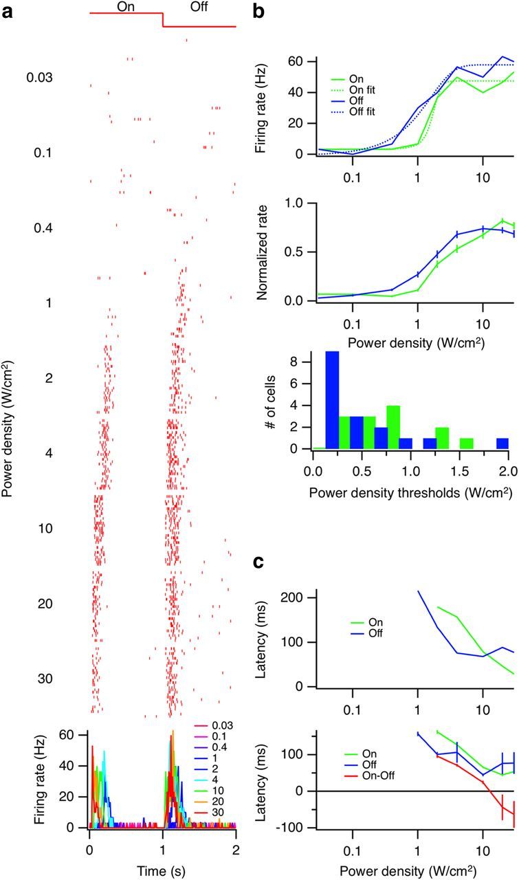
Dependence of response on US power density. a, Top, Raster plots of a single cell at increasing US power levels. Bottom, Superimposed PSTHs (10 ms bins). b, Top, Peak firing rates for On and Off responses for one cell versus power density (solid lines) along with sigmoid fits (dotted lines). Middle, Population summary, On (n = 29) and Off (n = 32) responses shown separately. The peak firing rate of each cell was normalized to its maximum rate. Error bars indicate SEM. Bottom, For cells that were fit well by sigmoid, a threshold was defined at 5% of the minimum–maximum range. A histogram of those thresholds is shown (On median = 754 mW/cm², Off median = 250 mW/cm², Wilcoxon-Mann-Whitney two-sample rank test: p = 0.0033, one-tailed). c, Top, Latencies to first spike for the example cell in a. Bottom, Population summary of average latencies. Error bars indicate SEM.

Comparing visual responses to US responses (simple periodic stimuli)

The responses of individual ganglion cells to an US stimulus (43 MHz) modulated at 0.5 Hz were strong and reproducible, much like visual responses to a 0.5 Hz flashing 100 μm spot that illuminated the same area as the US stimulus (Fig. 4a). For some cells, the firing rate and duration of the responses were similar, except that latency of the US response was shorter than visual latencies (Fig. 4a, middle and right). For other cells, US stimuli generated both ON and OFF responses, whereas visual stimuli generated only OFF responses (Fig. 4a, left).

Figure 4.

Precise, reproducible activation of the retina from US stimulation. a, Raster plots (30 trials) and PSTHs of three cells for both visual and US stimuli, 0.5 Hz, showing Off type (left), On-Off type (middle), and On type (right) ganglion cells. b, Ganglion cell recorded with a multielectrode array responding to a 0.5 Hz US stimulus. Top, Stimulus trace showing amplitude of US stimulus. Middle, Raster plot of spiking activity from repeated trials for a ganglion cell. Bottom, Expanded trace beginning at the offset of the US pulse. Periodic neural activity is consistent with refractoriness. c, Left, Comparison of US and visual latencies to first spike for cells in which the peak of the PSTH exceeds 25 Hz (On, correlation coefficient r = 0.34, p = 0.12; Off, r = 0.2, p = 0.2). Middle, Comparison of On and Off latencies for visual responses (r = 0.58, p = 0.0024) and for US responses (r = 0.75, p = 0.01). Right, Jitter was computed for each cell for US and visual responses as the SDs of the first spike latencies. Shown is a histogram of the ratio of US jitter to visual jitter for each cell (median = 0.88, paired t test p = 0.904). d, Ratio of power at the fundamental frequency (F1, 0.5 Hz) to power at the second harmonic (F2, 1.0 Hz) for US and visual stimuli (r = 0.006, p = 0.49).

We found that US stimulation produced precisely timed spikes across multiple repetitions (Fig. 4b). Transient bursts of action potentials occurred both at the onset and offset of the US pulse. For cells that responded to both visual and US stimulation, the latency of the US response was on average considerably shorter than the visual response (Fig. 4c, left, visual On, 139 ± 3.3 ms, US On, 98 ms ± 4.5 ms, two-tailed paired t test, p = 6.5 × 10⁻⁶, n = 14; visual Off, 111 ± 3.8 ms, US Off 49 ± 2.8 ms, two-tailed paired t test, p = 5.9 × 10⁻⁸, n = 19). It is likely that this latency difference arises because the US stimulus acts later in the circuit, at the very least bypassing the phototransduction cascade. For visual responses, latencies were longer for On than for Off responses, arising because On and Off signals are conveyed by different neural pathways containing On and Off bipolar cells, respectively. Similarly, US responses had a longer latency for On than Off responses, suggesting that two types of US responses also traveled through different neural pathways (Fig. 4c, middle).

The temporal precision of neural responses was similar across the population between US and visual stimuli (Fig. 4c, right) and in some cases was smaller than 1 ms, as has been reported for visual stimuli (Fig. 4b) (Berry et al., 1997) Thus, even though the latency was significantly shorter, the jitter was not significantly different (Fig. 4c, right, median = 0.88, paired t test, p = 0.904). This suggests that, under these visual stimulus conditions, the variability in latency is not substantially influenced by the phototransduction cascade, but by later circuit elements.

To measure the relative strength of On and Off responses, we analyzed the frequency response of cells to the US stimulus presented at 0.5 Hz. We compared the response at the fundamental (F1 = 0.5 Hz) frequency and at the second harmonic (F2 = 1 Hz). Cells that only respond to onset or offset will have a strong F1 component, whereas cells that respond equally strongly to both onset and offset will have a strong F2 but weak fundamental response. In 48% of cells, the ratio of the fundamental to the second harmonic was much less for US than for visual stimuli (Fig. 4d). This difference between US and visual responses suggested that US signals travel to some extent through different neural pathways than visual stimuli, therefore indicating that US stimuli in part activate cells other than photoreceptors. Further experiments and analyses to address this issue are presented below.

US mapping of receptive fields

We then measured the response to US stimuli as a function of distance from the ganglion cell. Retinal ganglion cells have a spatially antagonistic receptive field, with a surrounding area that responds to light with the opposite sign as the receptive field center. To measure whether this spatial antagonism was present in US responses, the transducer was moved in relatively large steps (350 μm), as the receptive field surround can extend to 1 mm radius. In the example shown in Figure 5a, the cell responded mostly to US Off when the stimulus was placed over the receptive field center (Fig. 5a, right and bottom, x = 0), but responded to US On only when the stimulus was moved 700 μm away (Fig. 5a, left and bottom, x = −0.7 mm). As is the case with visual stimuli, the antagonistic surround spanned a larger region than the receptive field center (Fig. 5b). This effect indicates processing within the retinal network, implying that US stimuli in part stimulated cells other than ganglion cells directly.

Figure 5.

US activates lateral retinal circuitry. a, Top, PSTHs from a single cell at two different locations of the US transducer. Bottom, Peak firing rate of the On and Off response as a function of distance from the cell's peak location of activation. b, Population summary (n = 19) showing the ratio of spatial On response width to the Off response width.

The neural code of US neurostimulation

Ganglion cell visual responses can be approximated by a model containing a linear temporal filter followed by a static nonlinearity (Baccus and Meister, 2002). In this LN model, the temporal filter represents the average change in firing rate in response to a brief pulse of light, and the nonlinearity is a time-independent function that captures the sensitivity, threshold, and any saturation in the response. To compute LN models, the US stimulus was modulated in time with binary noise. This was compared with a visual LN model computed by modulating a 100 μm spot visual stimulus with the same binary noise. The linear filter was calculated by the standard method of reverse correlation as the time-reverse of the average stimulus preceding a spike. After convolving the stimulus through this filter, a static nonlinearity was computed as the average instantaneous relationship between the filter output and firing rate (Fig. 6a). The filters were normalized in amplitude so that the total sensitivity was represented in the average slope of the nonlinearity.

Figure 6.

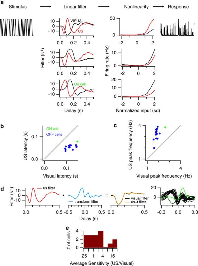
Comparing the neural code for US and visual stimuli. Top, LN models were computed using the standard method of reverse correlation with either the US stimulus or a 100 μm visual spot, both modulated with binary white noise. a, Examples of LN models for three cells, for both visual and US stimuli. b, Latency to first peak of the filter compared for visual and US stimuli (n = 15 from two retinas). Two cells were excluded whose temporal filters in visual and US stimuli had opposite sign. c, Peak modulation frequency computed from the Fourier transform of the filter. d, Far left, The US filter from the cell in the top row of a. Left middle, The optimal transform filter that transforms the US filter into the visual filter. Right middle, The transformed US filter (orange) compared with the visual filter (black, RMS difference between the two filters shown was 8.0%). Far right, All optimal filters that transform the US filters into the visual filters. Green represents the ON cell shown in the bottom of a; dark green, the cell in the second row of a. e, Average sensitivity for each US and visual condition was computed as the average slope of the nonlinearity. Histogram of ratios of US to visual sensitivity for each cell (median = 1.6, paired t test, p = 0.043).

US filters (Fig. 6a, left, red) had a much shorter latency and time to peak compared with visual filters, as expected from the shorter latency of periodic pulses of US stimuli (Fig. 4). US filters were also very strongly biphasic, even triphasic, meaning that they were differentiating or high-pass filters, reflecting transient responses. Other differences that were seen between US and visual filters observed occasionally were that the US filter had the opposite polarity from the visual filter (2 of 17 cells) (Fig. 6a, middle), or that the US and visual filter had similar dynamics, but a different latency (1 of 17 cells) (Fig. 6a, bottom).

Additional diversity was observed between visual and US nonlinearities (Fig. 6a, right). In general, the average sensitivity for the US response could be greater (7 of 16 cells) (Fig. 6a, top), less than (3 of 16 cells) (Fig. 6a, bottom), or approximately equal to (within a factor of 2, 6 of 16 cells) the sensitivity of the visual response. The average sensitivity for US and visual nonlinearities is compared in Figure 6e.

We then considered the hypothesis that US stimulated photoreceptors only and that the only difference from visual stimulation comes from bypassing the phototransduction cascade. If this were true, then the differences in the visual and US filters could be explained by another fixed linear, causal filter that did not vary from cell to cell. For that purpose, we summarized filter characteristics across the population in Figure 6b–d, looking at the time to first peak (Fig. 6b) and the peak stimulus frequency measured from the Fourier transform of the filter (Fig. 6c). For Off cells, visual latencies were more diverse than US latencies; there was not a single number to describe the difference.

Then for each cell, we explicitly computed the filter that would transform the US filter into the visual filter. This represented the temporal filtering bypassed by the US stimulus (Fig. 6d). We found that this transforming filter between US and visual stimuli varied across cells (Fig. 6d, right). Furthermore, it included a substantial acausal component (to the left of zero in Fig. 6d, far right), which was inconsistent with a single initial filtering step that was bypassed by the US stimulus. The average normalized root mean squared (RMS) difference between the transformed US filter and the visual filter was 19.9 ± 8.0% using an acausal filter. When the filter was constrained to be causal by setting it to be zero in the acausal direction, this RMS difference increases to 87.7 ± 13.8%, indicating that causal filter was insufficient. Thus, it is unlikely that US stimulated photoreceptors alone.

US modulation of visual responses

By applying both visual and US stimuli simultaneously, we measured how US modulates the normal processing of visual input. We used a visual stimulus composed of a binary random checkerboard, from which we computed the linear spatiotemporal filter, a single static nonlinearity, and the two dimensional spatial receptive field. During this visual stimulation we delivered a periodic US pulse of 200 ms duration every 2 s (Fig. 7a). The data was analyzed by correlating response to the visual stimulus, and was subdivided into three time intervals, 1) the 200 ms during which the US pulse was turned on (‘On’), 2) the 200 ms immediately after the US pulse was turned off (‘Off’), 3) a control period that extended from 300 ms after the pulse was turned off until the next pulse (‘Control’). The Off and Control periods were defined by first analyzing the response in multiple 200 ms intervals, and determining that these three time intervals were representative of the dynamic changes.

Figure 7.

US rapidly modulates visual responses. a, Visual stimulus was a binary random checkerboard presented simultaneously with a 0.2 s US pulse delivered every 2 s. Spikes were analyzed relative to the visual stimulus as in Equation 1 but subdivided into three time intervals according to the US stimulus: On, during the 0.2 s US stimulus; Off, up to 0.2 s immediately after US; and Control, 0.1 s after the Off interval until the next On interval. b, Firing rate (light blue), temporal filters, and nonlinearities for three cells. Colors are indicated in a. Three example cells are shown. c, Changes in threshold and average sensitivity of the nonlinearities caused by US (n = 35). Left, Change in average sensitivity, computed as the average slope of the nonlinearity, during US On versus during Off periods. Right, Change in threshold during On period versus Off period. d, Left, Receptive fields of 35 retinal ganglion cells. Red indicates the US focus. Middle left, Total visual sensitivity across the population. For each cell, sensitivity was computed at each spatial location as the RMS value of the spatiotemporal filter at that spatial location. Total sensitivity was computed by summing across all cells. Middle right, The change in sensitivity produced by US On computed as the total sensitivity during US On minus the total sensitivity during control. Red pixels indicate a reduction and blue pixels indicate an increase in sensitivity. Right, The change in sensitivity produced by US Off. e, Change in sensitivity as a function of distance from the US focus for On (left) and Off (right) intervals. A Gaussian fit during the Off interval has an SD of 110 μm.

At US onset or offset, many cells briefly changed their firing rate (Fig. 7b). However, during these changes in firing rate, there was virtually no change in the visual temporal filters, except in some cases noise increased because of a lower firing rate. Visual nonlinearities changed in accordance with the change in firing rate. Figure 7c compares changes in the threshold (lateral shift) and average sensitivity (vertical scaling) of the nonlinearity at US On and Off (Fig. 7c). Most cells (74%) showed increases in sensitivity both during the On and Off periods relative to the Control period, changes that were weakly correlated in the two time intervals (Fig. 7c, left, correlation coefficient r = 0.57, p = 0.00017). For less than half of the cells (43%, Fig 7c, right), threshold increased for both On and Off periods of US. Considerable diversity was observed in these changes in sensitivity and threshold. In summary, the US stimulus generally did not fundamentally change temporal filtering but did change threshold and sensitivity in a manner that greatly differed between cells.

Because the spatial visual stimuli enable a very localized measurement of visual sensitivity across a population of ganglion cells, we used the visual spatial receptive field maps to derive an upper limit on the spatial scale of the US stimulus. Figure 7d (far left) shows the spatial distribution of visual receptive fields relative to the US transducer location (red “+”). We first computed a spatial map of total visual sensitivity across the population of cells by summing the RMS amplitude of each cell's spatiotemporal receptive field for each spatial location (Fig. 7d, left middle). Then, for each cell, we calculated the slope of the nonlinearity as an estimate of the sensitivity for the three conditions (On, Off, Control). The amplitude of each receptive field was weighted by the change in sensitivity created by US On or Off conditions compared with Control, and these results were summed across all cells. This yielded a spatial map of the total change in sensitivity produced by US.

At the onset of US stimulation, regions near the transducer showed a reduction in sensitivity, whereas regions far away that experience an increase in sensitivity (Fig. 7d, middle right). For these distant cells, US likely stimulated the receptive field surround. At the offset of the US stimulus, we observed a spatially localized increase in sensitivity (Fig. 7d, far right). A summary of the average change in sensitivity as a function of distance from the US focus is shown in Figure 7e. A Gaussian fit to the effect at the offset of the US stimulus shows an SD of 110 μm, which can be considered an upper limit on the spatial resolution of the US transducer. This measure of resolution is affected by the lateral spread of the signal inherent in retinal circuitry, so the actual spatial scale of stimulation may be smaller.

Effects of US when synaptic transmission is blocked

The previous results imply that US stimuli are processed in retinal circuitry and that we are not exclusively stimulating ganglion cells directly. To directly measure the effect of US on ganglion cells, we blocked vesicular transmitter release. This was accomplished by perfusing the retina with 100 μm CdCl₂, and replacing Ca with Mg (Brivanlou et al., 1998). This yielded a higher than normal level of spontaneous activity, which was potentially useful in the detection of any decreases in activity. US stimulation at a stimulus frequency of 0.5 Hz was applied for 60 s. Before perfusing CdCl₂, we measured responses to the 100 μm visual spot and US stimuli at the normal power level (30 W/cm²) as a control to verify normal stimulation (Fig. 8a).

Figure 8.

CdCl₂ abolishes neurostimulation by US. a, Raster plots of three cells (columns) that responded well to visual and US stimuli in the control condition. Top and middle rows, Visual and US responses in the normal Ringer's solution. Bottom, US response during 100 μm CdCl₂, and Ca²⁺ replaced with Mg²⁺ (b) PSTHs of these three cells.

While perfusing CdCl₂, US stimulation (30 W/cm²) produced virtually no response (Fig. 8b). The stimulus was repeated at progressively higher-power levels up to 180 W/cm², but at no point did we obtain any stimulus-locked response; at most, there was some slow modulation of spontaneous activity (data not shown). We computed the sum of the fundamental and second harmonic of the response for 19 cells and found that none of these cells responded to US stimuli in the presence of CdCl₂ (response was 2.8 ± 1.5% of control). Thus, US neurostimulation does not appear to directly activate ganglion cells, and requires synaptic transmission. One possibility for this effect is that US stimulation of the retina either results in small membrane potential changes that require amplification by synapses before ganglion cells, or that the effect may be directly on synaptic release. In either case, the effect does not appear to be a general effect on the membrane or on all voltage-dependent ion channels.

We further tested whether US acted on photoreceptors alone by blocking synaptic transmission in the On pathway with L-AP4. Because L-AP4 acts selectively on the synaptic input to On bipolar cells, if US acted solely through photoreceptors, L-AP4 should also block US stimulation through the On pathway. We measured responses to both US and visual stimulation in the presence and absence of L-AP4 and found that all visual responses at the onset of light were suppressed by L-AP4 as expected. However, the response to the onset of US was in general unaffected by L-AP4 (Fig. 9a–c). When analyzing results across the population, however, we did observe a weak but significant correlation between the strength of the On response in the cell and the strength of the effect of APB (Fig. 9c, far right). Approximately 18% of the variance of the effect of APB could be accounted for by a difference in the strength of the On response (r² = 0.18, p = 0.0013, two-tailed). This indicates that, to a weaker extent, US also stimulates photoreceptors. Overall, we conclude that, because L-AP4 largely did not block the On response to US, a substantial part of the direct effect of US stimulation is on cells beyond photoreceptors.

Figure 9.

US acts in part downstream of the photoreceptor to bipolar cell synapse. a, Left, Raster plots and PSTHs for visual and US (20 W/cm²) responses in the control condition for an example cell. Middle, Raster plots and PSTHs after 30 min of 20 μm L-AP4 perfusion. Right, Raster plots and PSTHs after 60 min of washout. b, Left, Histogram of On suppression index for visual stimuli: n = 33 (−1, complete suppression of On response; 0, no effect; +1, an On response appears with drug that was not present during control). Right, Histogram of On suppression index for US stimuli; n = 63. The mean was not significantly different from zero (p = 0.85, t test). c, Left, Visual versus US suppression indices; n = 29 (different distributions: Wilcoxon Signed Rank, p = 1.2 × 10⁻⁷, two-tailed). Diagonal line indicates equal suppression. Right, On-Off index from visual control (+1, pure ON cell; −1, pure OFF cell) versus US suppression index. Black line indicates a linear fit.

Discussion

We have shown that US stimulation can be used to convey precise temporal information across a range of signals similar to natural visual input. The use of a high acoustic frequency further enables a fine lateral spatial resolution (∼100 μm), consistent with the maximum resolution of the 43 MHz frequency (Fig. 7). Furthermore, US stimulation both indirectly activates ganglion cells independent of visual stimulation and rapidly modulates sensitivity to natural visual input. With regard to the optimal stimulus parameters, we find high-frequency modulation to be unnecessary, neither beneficial nor detrimental. Low-frequency modulation was effective in the normal physiologic range equivalent to the natural visual stimulus.

US stimuli for clinical treatments and basic studies

For clinical use as a prosthesis, it is critical to deliver sensory information at a spatial and temporal resolution and range similar to that of natural visual input. Furthermore, this information must be delivered to existing neurons in the degenerated retina. Similarities between US and visual responses, and a center/surround receptive field structure measured with US (Fig. 5), all indicate that retinal circuitry processes the US signal. Furthermore, although US did not directly stimulate ganglion cells (Fig. 8) when synaptic transmission was blocked, it did activate cells beyond photoreceptors (Fig. 9). Finally, because many patients with retinal disease may have some existing natural vision, it is important to understand how US stimuli modulate visual sensitivity. Although US modulates visual sensitivity (Fig. 7), these effects are highly localized. Our results indicate that ultrasonic neurostimulation of the retina may be useful in a clinical setting for diagnosis of retinal health in the absence of intact photoreceptors, and potentially as a noninvasive retinal prosthesis.

For basic studies of neural circuits, although each artificial stimulus method has limitations in spatiotemporal resolution or cellular specificity, these might be overcome by combinations with other methods. In particular, extracellular methods of stimulation often lack specificity in terms of cell types. By combining US stimuli with specific pharmacology, as we have done (Figs. 8 and 9), one could potentially understand the effects of pharmacologically defined neural pathways with the spatiotemporal specificity of the US stimulus.

Likely mechanisms of US neurostimulation

This combination of US and pharmacology has revealed new information about the potential biophysical mechanism of US stimuli. Because US stimuli do not directly change the firing rate of ganglion cells (Fig. 8), this argues against a nonspecific effect on all cells, such as a transient disruption of the cellular membrane. Another potential mechanism is an effect on voltage-dependent or mechanosensitive ion channels, but only if these effects are specific to different cell types, either resulting from their set of ion channels or their cellular geometry. A final possibility is a direct effect on the presynaptic terminal. If so, this effect must be felt at or before the step of Ca influx. If the effect were direct upon the machinery of vesicle fusion subsequent to the effect of Ca²⁺, it would likely not be sensitive to Cd⁺.

Interpretation of retinal processing

Given that US acts in part on cells beyond photoreceptors, we can use this knowledge to interpret the origin of certain aspects of neural signaling, one example being the source of variability in retinal processing. It is known that, for strong visual stimuli, the temporal precision of ganglion cells can exceed 1 ms (Berry et al., 1997). However, the retinal elements that establish this limit on temporal precision are unknown. It is thought that the major source of noise in the retina comes from photoreceptors (Ala-Laurila et al., 2011), although these conclusions come from analyzing the statistics of single photoreceptors. We have found, however, that although US responses have a much shorter latency, they do not have less variability under the stimulus conditions we tested (Fig. 4). Thus, under the stimulus conditions of a strong flashing spot, noise in photoreceptors does not seem to have the dominant influence over ganglion cell variability. One explanation is that, when multiple photoreceptors receive the same stimulus, as will occur in the case of many natural photopic stimuli, independent noise in photoreceptors is reduced through signal averaging and downstream noise in interneuron transmission or ganglion cell spike generation has a greater influence on temporal variability.

A second aspect revealed through the use of US stimuli involves prolonged dynamics in temporal filtering (Fig. 6). Although US stimuli are of shorter latency, consistent with stimuli that bypass the phototransduction cascade (Baylor and Fettiplace, 1977; Ala-Laurila et al., 2011), they nonetheless have prolonged dynamics. This supports the idea that circuit elements downstream of photoreceptors have a significant influence on temporal filtering, as has been suggested from current injection in inhibitory amacrine cells (de Vries et al., 2011).

Finally, we observed a modulation of visual sensitivity that occurs without a change in temporal filtering, as has been observed from direct current injection into sustained amacrine cells (de Vries et al., 2011). This supports the idea that the control of sensitivity and temporal filtering are to some extent independent.

Toward high-resolution patterned US neurostimulation

Early experiments demonstrated the effectiveness of US suppression of neural activity in visual cortex or peripheral nerve but not for generating activity (Fry et al., 1958; Young and Henneman, 1961) However, an early study in cat and rabbit brain indicated that neural excitation occurred at relatively lower US power levels, whereas higher-power levels produced suppression (Velling and Shklyaruk, 1988). In experiments with frog sciatic nerve, US stimulation at high power decreased compound action potential amplitudes elicited by electrical stimulation, an effect that was attributed to increases in temperature (Tsui et al., 2005). Lower power, however, did create a small enhancement (8%) in amplitude, which did not appear to be the result of temperature.

Recent studies, however, have demonstrated the potential for US to generate neural activity. Low-intensity, unfocused US stimulated neurons in mouse hippocampal slices and mouse brains (Tyler et al., 2008). Low-power US stimulated motor cortex in mice as measured by local field potentials and multiunit activity in primary motor cortex (Tufail et al., 2010). Although these studies clearly demonstrate neurostimulation, there was little control over the spatial extent of the stimulation, which was generally quite large (∼2 mm lateral). In a similar study using “focused” US that activated rabbit motor cortex measured by fMRI and behavior, the size of the acoustic focus was estimated to be 2.3 mm in diameter and 5.5 mm in length (Yoo et al., 2011). Finally, recent work has shown the feasibility of in vivo retinal stimulation (Naor et al., 2012) .

For both clinical applications and for use in the study of the retinal circuit, higher US frequencies and an array of focused transducers will be useful to achieve single-cell stimulation. Recent theoretical work has examined the possibility of producing patterned ultrasonic neurostimulation in the retina (Hertzberg et al., 2010). Capacitive micro-machined ultrasonic transducer arrays can operate in the same acoustic frequency range used in the present study (Oralkan et al., 2004; Yeh et al., 2005). We expect that development of such arrays will allow similar spatial resolution and focal intensity for precise spatiotemporal patterned neurostimulation.

References

- Ala-Laurila P, Greschner M, Chichilnisky EJ, Rieke F. Cone photoreceptor contributions to noise and correlations in the retinal output. Nat Neurosci. 2011;14:1309–1316. doi: 10.1038/nn.2927. [DOI] [PMC free article] [PubMed] [Google Scholar]
- Baccus SA, Meister M. Fast and slow contrast adaptation in retinal circuitry. Neuron. 2002;36:909–919. doi: 10.1016/s0896-6273(02)01050-4. [DOI] [PubMed] [Google Scholar]
- Baylor DA, Fettiplace R. Kinetics of synaptic transfer from receptors to ganglion cells in turtle retina. J Physiol. 1977;271:425–448. doi: 10.1113/jphysiol.1977.sp012007. [DOI] [PMC free article] [PubMed] [Google Scholar]
- Berry MJ, Warland DK, Meister M. The structure and precision of retinal spike trains. Proc Natl Acad Sci U S A. 1997;94:5411–5416. doi: 10.1073/pnas.94.10.5411. [DOI] [PMC free article] [PubMed] [Google Scholar]
- Brivanlou IH, Warland DK, Meister M. Mechanisms of concerted firing among retinal ganglion cells. Neuron. 1998;20:527–539. doi: 10.1016/s0896-6273(00)80992-7. [DOI] [PubMed] [Google Scholar]
- Chichilnisky EJ. A simple white noise analysis of neuronal light responses. Network. 2001;12:199–213. [PubMed] [Google Scholar]
- Chou CH, Khuri-Yakub BT, Kino GS. Lens design for acoustic microscopy. IEEE Trans Ultrason Ferroelectr Freq Control. 1988;35:464–469. doi: 10.1109/58.4183. [DOI] [PubMed] [Google Scholar]
- Clement GT, White PJ, King RL, McDannold N, Hynynen K. A magnetic resonance imaging-compatible, large-scale array for trans-skull ultrasound surgery and therapy. J Ultrasound Med. 2005;24:1117–1125. doi: 10.7863/jum.2005.24.8.1117. [DOI] [PubMed] [Google Scholar]
- de Vries SE, Baccus SA, Meister M. The projective field of a retinal amacrine cell. J Neurosci. 2011;31:8595–8604. doi: 10.1523/JNEUROSCI.5662-10.2011. [DOI] [PMC free article] [PubMed] [Google Scholar]
- Fry FJ, Ades HW, Fry WJ. Production of reversible changes in the central nervous system by ultrasound. Science. 1958;127:83–84. doi: 10.1126/science.127.3289.83. [DOI] [PubMed] [Google Scholar]
- Hertzberg Y, Naor O, Volovick A, Shoham S. Towards multifocal ultrasonic neural stimulation: pattern generation algorithms. J Neural Eng. 2010;7 doi: 10.1088/1741-2560/7/5/056002. 056002. [DOI] [PubMed] [Google Scholar]
- Histed MH, Ni AM, Maunsell JHR. Insights into cortical mechanisms of behavior from microstimulation experiments. Prog Neurobiol. 2012 doi: 10.1016/j.pneurobio.2012.01.006. Advance online publication. Retrieved Jan. 28, 2012. [DOI] [PMC free article] [PubMed] [Google Scholar]
- Kalanithi PS, Henderson JM. Optogenetic neuromodulation. Int Rev Neurobiol. 2012;107:185–205. doi: 10.1016/B978-0-12-404706-8.00010-3. [DOI] [PubMed] [Google Scholar]
- Krasovitski B, Frenkel V, Shoham S, Kimmel E. Intramembrane cavitation as a unifying mechanism for ultrasound-induced bioeffects. Proc Natl Acad Sci U S A. 2011;108:3258–3263. doi: 10.1073/pnas.1015771108. [DOI] [PMC free article] [PubMed] [Google Scholar]
- Liang K, Khuri-Yakub B, Bennett S, Kino G. Phase measurements in acoustic microscopy. Proc IEEE Ultrason Symp. 1983:599–604. [Google Scholar]
- Naor O, Hertzberg Y, Zemel E, Kimmel E, Shoham S. Towards multifocal ultrasonic neural stimulation: II. Design considerations for an acoustic retinal prosthesis. J Neural Eng. 2012;9 doi: 10.1088/1741-2560/9/2/026006. 026006. [DOI] [PubMed] [Google Scholar]
- Oralkan O, Hansen ST, Bayram B, Yaralglu GG, Ergun AS, Khuri-Yakub BT. High-frequency CMUT arrays for high-resolution medical imaging. Proc IEEE Ultrason Symp. 2004;1:399–402. [Google Scholar]
- Rossini PM, Rossi S. Transcranial magnetic stimulation: diagnostic, therapeutic, and research potential. Neurology. 2007;68:484–488. doi: 10.1212/01.wnl.0000250268.13789.b2. [DOI] [PubMed] [Google Scholar]
- Tsui PH, Wang SH, Huang CC. In vitro effects of ultrasound with different energies on the conduction properties of neural tissue. Ultrasonics. 2005;43:560–565. doi: 10.1016/j.ultras.2004.12.003. [DOI] [PubMed] [Google Scholar]
- Tufail Y, Matyushov A, Baldwin N, Tauchmann ML, Georges J, Yoshihiro A, Tillery SI, Tyler WJ. Transcranial pulsed ultrasound stimulates intact brain circuits. Neuron. 2010;66:681–694. doi: 10.1016/j.neuron.2010.05.008. [DOI] [PubMed] [Google Scholar]
- Tyler WJ. Noninvasive neuromodulation with ultrasound? A continuum mechanics hypothesis. Neuroscientist. 2011;17:25–36. doi: 10.1177/1073858409348066. [DOI] [PubMed] [Google Scholar]
- Tyler WJ, Tufail Y, Finsterwald M, Tauchmann ML, Olson EJ, Majestic C. Remote excitation of neuronal circuits using low-intensity, low-frequency ultrasound. PLoS One. 2008;3:e3511. doi: 10.1371/journal.pone.0003511. [DOI] [PMC free article] [PubMed] [Google Scholar]
- Velling VA, Shklyaruk SP. Modulation of the functional state of the brain with the aid of focused ultrasonic action. Neurosci Behav. Physiol. 1988;18:369–375. doi: 10.1007/BF01193880. [DOI] [PubMed] [Google Scholar]
- Yeh D, Oralkan O, Wygant I, Ergun A, Wong J, Khuri-Yakub B. High-resolution imaging with high-frequency 1-D linear CMUT arrays. Proc IEEE Ultrason Symp. 2005;1:665–668. [Google Scholar]
- Yoo SS, Bystritsky A, Lee JH, Zhang Y, Fischer K, Min BK, McDannold NJ, Pascual-Leone A, Jolesz FA. Focused ultrasound modulates region-specific brain activity. Neuroimage. 2011;56:1267–1275. doi: 10.1016/j.neuroimage.2011.02.058. [DOI] [PMC free article] [PubMed] [Google Scholar]
- Young RR, Henneman E. Functional effects of focused ultrasound on mammalian nerves. Science. 1961;134:1521–1522. doi: 10.1126/science.134.3489.1521. [DOI] [PubMed] [Google Scholar]