Rubik: Knowledge Guided Tensor Factorization and Completion for Health Data Analytics

Abstract

Computational phenotyping is the process of converting heterogeneous electronic health records (EHRs) into meaningful clinical concepts. Unsupervised phenotyping methods have the potential to leverage a vast amount of labeled EHR data for phenotype discovery. However, existing unsupervised phenotyping methods do not incorporate current medical knowledge and cannot directly handle missing, or noisy data.

We propose Rubik, a constrained non-negative tensor factorization and completion method for phenotyping. Rubik incorporates 1) guidance constraints to align with existing medical knowledge, and 2) pairwise constraints for obtaining distinct, non-overlapping phenotypes. Rubik also has built-in tensor completion that can significantly alleviate the impact of noisy and missing data. We utilize the Alternating Direction Method of Multipliers (ADMM) framework to tensor factorization and completion, which can be easily scaled through parallel computing. We evaluate Rubik on two EHR datasets, one of which contains 647,118 records for 7,744 patients from an outpatient clinic, the other of which is a public dataset containing 1,018,614 CMS claims records for 472,645 patients. Our results show that Rubik can discover more meaningful and distinct phenotypes than the baselines. In particular, by using knowledge guidance constraints, Rubik can also discover sub-phenotypes for several major diseases. Rubik also runs around seven times faster than current state-of-the-art tensor methods. Finally, Rubik is scalable to large datasets containing millions of EHR records.

1. INTRODUCTION

The widespread adoption of EHR systems in the United States and many other countries has resulted in a tsunami of EHR data, which is becoming an increasingly important source of detailed medical information. Successful phenotyping efforts on EHR data can enable many important applications, such as clinical predictive modeling [12, 27] and EHR-based genomic association studies [12, 17, 27]. Furthermore, medical professionals are accustomed to reasoning based on concise and meaningful phenotypes. Thus, it is imperative that robust phenotyping methods be developed and refined to keep up with the growing volume and heterogeneity of EHR data.

A typical phenotyping algorithm takes EHR data as input, and defines a group or several groups of patients, each of which is referred to as a phenotype. An example of a phenotype is shown in Table 1, which depicts a collection of diseases and associated medications that may co-occur in a patient¹. In Table 1 and in all subsequent displays of phenotypes throughout the paper, the diagnoses and medications are shown by rank order of importance.

Table 1:

An example of a phenotype that a group of patients may exhibit. The diagnoses and medications are shown in rank order of importance.

Diagnoses	Medications
Hypertension	Statins
Ischemic heart disease	Angiotensin receptor blockers
Hyperlipidemia	ACE inhibitors
Obesity	Loop diuretics
	Cardioselective beta blockers

Most existing phenotyping methods are supervised approaches, which are either expert-defined rule-based methods [16] or classification methods [8]. However, as labeled data are difficult to obtain, efficient unsupervised phenotyping approaches are needed to leverage the vast amount of unlabeled EHR data for discovering multiple interconnected phenotypes. The only such algorithm to our knowledge is based on sparse nonnegative tensor factorization [14, 15], which models interconnected data as tensors and discovers sparse nonnegative factors as phenotypes. However, there are still several formidable challenges in unsupervised phenotyping methods:

• Leverage of existing knowledge. Existing medical knowledge, such as a physician’s experience or a medical ontology, should be incorporated into the phenotyping algorithms in order to identify more meaningful phenotypes that align more closely with existing medical knowledge.

• Deriving distinct phenotypes. Existing unsupervised phenotyping methods, such as Marble [15], can lead to overlapping phenotypes which hinder their interpretation. Ideally, the resulting phenotypes should be distinct without much overlap.

• Missing and noisy data. EHR data often contain missing and noisy records. It is important to ensure that phenotyping algorithms remain robust against missing and noisy data.

• Scalability. Real world EHR data contains millions of records and spans multiple dimensions. It is important to develop innovative phenotyping methods that scale well with increases in data size.

Contributions: We propose Rubik, an unsupervised phenotyping method based on tensor factorization and completion, which addresses all the aforementioned challenges:

• We incorporate guidance constraints based upon medical knowledge in order to derive clinically meaningful phenotypes.

• We introduce pairwise constraints in the formulation to ensure distinct phenotypes.

• Our proposed algorithm embeds efficient tensor completion, thereby alleviating both missing and noisy information in EHR tensors.

• We design a scalable algorithm based on Alternating Direction Method of Multipliers (ADMM) for solving this problem, which significantly outperforms several baseline methods.

We evaluate Rubik on two large EHR datasets. Our results demonstrate that Rubik achieves at least a 60% reduction in the number of overlapping phenotypes compared to Marble as a baseline [15]. Rubik also increases the number of meaningful phenotypes by 50%. Furthermore, the phenotypes and the baseline characteristics derived from the real EHR data are consistent with existing studies on the population. Rubik is also much more computationally scalable compared to all baseline methods, with up to a 7-fold decrease in running time over the baselines.

Table 2 compares the properties between our model and other tensor methods.

Table 2:

A comparison of different tensor models

Property	Marble [15]	FaLRTC [22]	CTMF [2]	TF-BPP [18]	WCP [1]	NETWORK [10]	Rubik
Factorization	✓		✓	✓	✓	✓	✓
Completion		✓			✓		✓
Non-negativity	✓			✓			✓
Guidance						✓	✓
Sparse solution	✓						✓
Scalability							✓

Outline:

The remainder of the paper is organized as follows. We review preliminaries in Sec. 2. We present our framework in Sec. 3. Datasets and experimental evaluation are discussed in Sec. 4. Related work is summarized in Sec. 5. Finally, we conclude by discussing future research directions.

2. PRELIMINARIES

This section describes the preliminaries of tensor factorization. Table 3 defines symbols commonly used in the paper.

Table 3:

Common symbols used throughout the paper.

Symbol	Description
$\odot$	Khatri-Rao product
◦	outer product
*	element-wise product
N	number of modes
R	number of latent phenotypes
$\mathcal{X}$, $\mathcal{O}$	tensor
A,B	matrix
Ak	kth column of A
u, v	vector
$\overrightarrow{i}$	tensor element index (i1, i2,···, iN)
$\mathcal{X}\left(\overrightarrow{i}\right)$	tensor element at index $\overrightarrow{i}$
X(n)	mode-n matricization of tensor $\mathcal{X}$

Definition 1. A rank-one N^th order tensor $\mathcal{X}$ is the outer product of N vectors, a⁽¹⁾ ◦ a⁽²⁾ ◦ · · · ◦ a^(N), where each element ${\mathcal{X}}_{\overrightarrow{i}}=\mathcal{X}\left(i_1,i_2,\cdots ,i_N\right)=a_{i_1}^{\left(1\right)}{a}_{i_2}^{\left(2\right)}\cdots a_{i_N}^{\left(N\right)}$.

Definition 2. The Kronecker product of two matrices A ⊗ B of sizes I_A × R and I_B × R respectively, produces a matrix of size I_AI_B × R²

$$\mathbf{A}\otimes \mathbf{B}=\left[\begin{array}{ccc}{a}_{11}\mathbf{B}& \cdots & a_{1R}\mathbf{B}\\ ⋮& \ddots & ⋮\\ a_{I_{a}1}\mathbf{B}& \cdots & a_{I_{A}R}\mathbf{B}\end{array}\right]$$

Definition 3. Khatri Rao product of two matrices $\mathbf{A}\odot \mathbf{B}$ of sizes I_a × R and I_B × R respectively, produces a matrix C of size I_aI_b × R such that C = [a₁ ⊗ b₁ · · · a_R ⊗ b_R].

Definition 4. The mode-n matricization of $\mathcal{X}$, denoted by $X_{\left(n\right)}\in {ℝ}^{I_n\times \left(I_1\cdots I_{n-1}{I}_{n+1}{I}_N\right)}$ is the process of reordering the elements of a N -way array into a matrix.

Definition 5. The CANDECOMP-PARAFAC (CP) approach approximates the original tensor χ as a sum of rank-one tensors and is expressed as

$$\mathcal{X}\approx \sum _{r=1}^R{\mathbf{A}}_r^{\left(1\right)}\circ \cdots \circ {\mathbf{A}}_r^{\left(N\right)}=〚{\mathbf{A}}^{\left(1\right)};\cdots ;{\mathbf{A}}^{\left(N\right)}〛$$

where ${\mathbf{A}}_r^{\left(n\right)}$ corresponds to the r^th column of A⁽ⁿ⁾. We call ${\mathbf{A}}^{\left(1\right)},\cdots ,{\mathbf{A}}^{\left(N\right)}$ the factor matrices and use $〚\cdot 〛$ for a short-hand notation of the sum of rank-one tensors.

3. RUBIK

We first formulate the problem and then provide a general overview of the formulation. Finally, we present an efficient optimization algorithm for solving the problem.

3.1. Formulation

We formulate our model as a constrained tensor optimization, where four constraints (one hard and three soft) are involved:

• Completion: This is the hard constraint. The unknown full tensor $\mathcal{X}$ matches the observed elements in the partially observed tensor $\mathcal{O}$.

• Guidance: A subset of columns in a factor matrix A^(p) are close to the columns represented by prior knowledge ${\widehat{\mathbf{A}}}^{\left(p\right)}$.

• Pairwise constraints: The columns in a factor matrix A^(k) should be close to orthogonal.

• Non-negativity: The factor matrices A⁽¹⁾, …, A^(N) contain only nonnegative entries to enhance interpretability.

• Sparsity: We adjust the sparsity of each factor matrix A⁽ⁿ⁾ by removing non-zero entries less than γ_n.

$$\underset{\mathcal{X},\mathcal{T},\mathcal{C}}{\min }\left\{\mathbf{\Phi }\left(\mathcal{X},\mathcal{T},\mathcal{C}\right)\right\}, \text{s}.\text{t}.\underset{\text{Completion}}{\underbrace{{\mathcal{P}}_{\mathrm{\Omega }}\left(\mathcal{X}\right)={\mathcal{P}}_{\mathrm{\Omega }}\left(\mathcal{O}\right)}}$$

where,

$$\begin{gathered} \mathbf{\Phi }=\underset{\text{Factorization error}}{\underbrace{{\Vert \mathcal{X}-\mathcal{C}-\mathcal{T}\Vert }_F^2}}+\frac{{\lambda }_a}{2}\underset{\text{Guidance information}}{\underbrace{{\Vert \left({\mathbf{A}}^{\left(p\right)}-{\widehat{\mathbf{A}}}^{\left(p\right)}\right)\text{W}\Vert }_F^2}} \\ \hspace{1em}\hspace{1em}+\frac{{\lambda }_q}{2}\underset{\text{Pairwise constraint}}{\underbrace{{\Vert \mathbf{Q}-{\mathbf{A}}^{\left(k\right)T}{\mathbf{A}}^{\left(k\right)}\Vert }_F^2}} \\ \underset{\text{Interaction tensor}}{\underbrace{\mathcal{T}=〚{\mathbf{A}}^{\left(1\right)};\cdots ;{\mathbf{A}}^{\left(N\right)}〛\in {\mathrm{\Omega }}_{\mathcal{T}}}},\hspace{0.17em}\hspace{0.17em}\underset{\text{Bias tensor}}{\underbrace{\mathcal{C}=〚{\mathbf{u}}^{\left(1\right)};\cdots ;{\mathbf{u}}^{\left(N\right)}〛\in {\mathrm{\Omega }}_{\mathcal{C}}}} \\ {\mathrm{\Omega }}_{\mathcal{T}}={\mathrm{\Omega }}_{A_1}\times \cdots \times {\mathrm{\Omega }}_{A_N},{\mathrm{\Omega }}_{A_N}=\underset{\text{Sparse representation}}{\underbrace{\left\{\mathbf{A}\in \left\{0\right\}\cup {\left[{\gamma }_n,+\infty \right)}^{I_n\times R}\right\}}} \\ {\mathrm{\Omega }}_{\mathcal{C}}={\mathrm{\Omega }}_{u_1}\times \cdots \times {\mathrm{\Omega }}_{u_N},{\mathrm{\Omega }}_{u_n}=\left\{\mathbf{u}\in {\left[0,+\infty \right)}^{I_n\times 1}\right\} \end{gathered}$$ (1)

Next, we formally define all the necessary notations in Table 4.

Table 4:

Notations for Rubik

Notation	Definition
$\mathcal{X}\in {ℝ}_{+}^{I_1\times \cdots \times I_N}$	unknown full tensor partially observed tensor the set of observed indices set all but elements in Ω to zero
$\mathcal{O}\in {ℝ}_{+}^{I_1\times \cdots \times I_N}$
Ω
${\mathcal{P}}_{\mathrm{\Omega }}$
$\mathcal{X}\approx \mathcal{C}+\mathcal{T}$	$\mathcal{C}$: rank-one bias tensor
	$\mathcal{T}$: rank-R interaction tensor2
${\widehat{\mathbf{A}}}^{\left(p\right)}\in {ℝ}_{+}^{{}^{I_p\times R}}$	guidance matrix on mode-p pairwise constraint matrix weight matrix for guidance constraints
$\mathbf{Q}\in {ℝ}_{+}^{R\times R}$
$\mathbf{W}\in {\mathcal{R}}^{R\times R}$

In particular, the unknown full tensor $\mathcal{X}$ is approximated by two terms, 1) a rank one bias tensor $\mathcal{C}$ and 2) a rank-R interaction tensor $\mathcal{T}$. The bias tensor $\mathcal{C}$ captures the base-line characteristics of the entire tensor, which is a rank-one tensor with all positive vectors $〚{\mathbf{u}}^{\left(1\right)},\cdots ,{\mathbf{u}}^{\left(N\right)}〛$. The interaction tensor $\mathcal{T}$ is a CP tensor model, with nonnegative constraints on all factor matrices. Let $\mathbf{Q}\in {ℝ}_{+}^{R\times R}$ denote the pairwise constraints for a specific factor matrix say A^(k) with positive λ_q capturing the weights of this constraint. In our experiments, we set Q to be an identity matrix. The guidance knowledge is encoded as a vector where positive entries indicate relevant feature dimensions. For example, we can have a guidance vector corresponding to a hypertension diagnosis, where the hypertension-related entries are set to positive values (e.g., one), and the remaining entries are zero. Now, let us assume that we have R′ guidance vectors (R′ ≤ R). To ease subsequent derivation, we construct the guidance matrix ${\widehat{\mathbf{A}}}^{\left(p\right)}$ by adding zero columns to make ${\widehat{\mathbf{A}}}^{\left(p\right)}$ of the same size as the corresponding factor matrix ${\mathbf{A}}^{\left(p\right)}\in {ℝ}_{+}^{I_p\times R}$. Then, to ignore the effects of those zero columns, we multiply the difference between A^(p) and ${\widehat{\mathbf{A}}}^{\left(p\right)}$ by a weight matrix

$$\text{W=}\left(\begin{array}{cc}I& 0\\ 0& 0\end{array}\right)$$

where $I\in {ℝ}^{R^{\prime }\times R^{\prime }}$ is the identity matrix.

Next, we explain the intuition behind the model.

3.2. Problem Overview

At a high-level, Rubik aims to simultaneously conduct the non-negative CP factorization and recover the non-negative low rank tensor $\mathcal{X}$ from a partially observed tensor $\mathcal{O}$. This idea is captured through the Factorization error and Completion term in Eq. 1. Note that each ${\mathbf{A}}^{\left(k\right)}\in {ℝ}_{+}^{I_k\times R}$ has an estimated rank of R. Hence the interaction tensor $\mathcal{T}$ has rank up to R and the low rank property is enforced.

Bias tensor.

Rubik includes a rank-one bias tensor $\mathcal{C}$ to capture the baseline characteristics common in the overall population, which is similar to Marble [15]. In phenotyping applications, it represents the common characteristics of the n^th phenotype amongst the entire population (e.g., the value of the element in the diagnosis mode of the bias tensor corresponding to hypertension represents the overall possibility of any given patient having hypertension).

Guidance information.

In real world applications, we may know guidance information that can be encoded into the corresponding factor matrices. For example, we might have the knowledge that some phenotypes should be related to hypertension. Utilizing this guidance information can lead to more intuitive and understandable phenotypes. This constraint is captured through the Guidance information term in Eq. 1.

Pairwise constraints.

We hope to discover distinct phenotypes in order to obtain more concise and interpretable results. We can penalize the cases where phenotypes have overlapping dimensions (e.g., two common diagnoses between two phenotype candidates from the diagnosis mode). This constraint is captured through the Pairwise constraint term in Eq. 1.

3.3. Algorithm

Next we describe the detailed algorithm. The main idea is to decouple constraints using an Alternating Direction Method of Multipliers (ADMM) scheme [4]. For each mode, the algorithm first computes the factor matrix associated with the interaction tensor. Once the interaction factor matrix is computed, the bias vector is computed. The whole process is repeated until convergence occurs.

3.3.1. Convex Subproblem

Originally, the objective function Φ is non-convex with respect to A^(k) due to the fourth order term in pairwise constraints ${\Vert \mathbf{Q}-{\mathbf{A}}^{\left(k\right)T}{\mathbf{A}}^{\left(k\right)}\Vert }_F^2$. By variable substitution A^(k) = B^(k) in ${\Vert \mathbf{Q}-{\mathbf{A}}^{\left(k\right)T}{\mathbf{A}}^{\left(k\right)}\Vert }_F^2$ from Eq. 1, we obtain the equivalent form of Φ

$$\begin{gathered} \mathbf{\Psi }={\Vert \mathcal{X}-\mathcal{C}-\mathcal{T}\Vert }_F^2+\frac{{\lambda }_a}{2}{\Vert \left({\mathbf{A}}^{\left(p\right)}-{\widehat{\mathbf{A}}}^{\left(p\right)}\right)\mathbf{W}\Vert }_F^2 \\ \hspace{1em}\hspace{0.17em}\hspace{0.17em}\hspace{0.17em}+\frac{{\lambda }_q}{2}{\Vert \mathbf{Q}-{\mathbf{B}}^{\left(k\right)T}{\mathbf{A}}^{\left(k\right)}\Vert }_F^2 \end{gathered}$$

Note that the objective function Ψ is now convex w.r.t. A^(k).

Using a similar variable substitution technique, Eq. 1 is reformulated into the following equivalent form:

$$\begin{gathered} \hspace{1em}\hspace{1em}\hspace{1em}\underset{\mathcal{X},\mathcal{T},\mathcal{C},\mathcal{B},\mathcal{V}}{\min }\left\{\mathbf{\Psi }\right\} \\ \text{s}.\text{t}.\hspace{0.17em}{\mathbf{B}}^{\left(k\right)}={\mathbf{A}}^{\left(k\right)},{\mathbf{B}}^{\left(k\right)}\in {\mathrm{\Omega }}_{An},n=1,\cdots ,N \\ \hspace{1em}\hspace{0.17em}\hspace{0.17em}{\mathbf{v}}^{\left(n\right)}={\mathbf{u}}^{\left(n\right)}, {\mathbf{v}}^{\left(n\right)}\in {\mathrm{\Omega }}_{un},n=1,\cdots ,N \\ \hspace{1em}\hspace{0.17em}\hspace{0.17em}{\mathcal{P}}_{\mathrm{\Omega }}\left(\mathcal{X}\right)={\mathcal{P}}_{\mathrm{\Omega }}\left(\mathcal{O}\right) \end{gathered}$$ (2)

where $B=\left\{{\mathbf{B}}^{\left(1\right)},\cdots ,{\mathbf{B}}^{\left(N\right)}\right\}$ and $\mathcal{V}=\left\{{\mathbf{v}}^{\left(1\right)},\cdots ,{\mathbf{v}}^{\left(N\right)}\right\}$ are the collections of auxiliary variables.

3.3.2. Solving Scheme

The partial augmented Lagrangian function for Ψ is:

$$\begin{gathered} \mathcal{L}=\mathbf{\Psi }+\sum _{n=1}^N\left(\langle {\mathbf{p}}^{\left(n\right)},{\mathbf{v}}^{\left(n\right)}-{\mathbf{u}}^{\left(n\right)}\rangle +\frac{\eta }{2}{\Vert {\mathbf{v}}^{\left(n\right)}-{\mathbf{u}}^{\left(n\right)}\Vert }_F^2\right) \\ \hspace{1em}\hspace{1em}+\sum _{n=1}^N\left(\langle {\mathbf{Y}}^{\left(n\right)},{\mathbf{B}}^{\left(n\right)}-{\mathbf{A}}^{\left(n\right)}\rangle +\frac{\mu }{2}{\Vert {\mathbf{B}}^{\left(n\right)}-{\mathbf{A}}^{\left(n\right)}\Vert }_F^2\right) \end{gathered}$$ (3)

where $\mathcal{Y}=\left\{{\mathbf{Y}}^{\left(1\right)},\cdots ,{\mathbf{Y}}^{\left(N\right)}\right\}$ and $\mathcal{P}=\left\{{\mathbf{p}}^{\left(1\right)},\cdots ,{\mathbf{p}}^{\left(N\right)}\right\}$ are the set of Lagrange multipliers. $\langle X,Y\rangle ={\sum }_{ij}{X}_{ij}{Y}_{ij}$ denotes the inner product of two matrices X and Y. {η, μ} are penalty parameters, which can be adjusted efficiently according to [21].

Here we solve Eq. 3 by successively minimizing the Lagrangian with respect to each variable in block coordinate descent procedures. Each iteration involves updating one variable, with the other variables fixed to their most recent values. The updating rules are as follows.

Update the interaction tensor.

Without loss of generality, we assume that the prior and pairwise guidance information are on the n^th mode. One can easily modify λ_a; λ_q to zero if there is no guidance information on a particular mode. Set $\mathcal{R}=\mathcal{X}-\mathcal{C}$, which is the residual tensor left over after subtracting the effects of the bias tensor in objective function Ψ. To compute ${\mathbf{A}}_{t+1}^{\left(n\right)}$, the smooth optimization problem is formulated as follows:

$$\begin{gathered} \underset{{\mathbf{A}}^{\left(n\right)}}{\min }{\Vert {\mathbf{A}}^{\left(n\right)}{\mathbf{\Pi }}^{\left(n\right)T}-{\mathbf{R}}_{\left(n\right)}\Vert }_F^2 \\ +\frac{{\lambda }_q}{2}{\Vert \mathbf{Q}-{\mathbf{B}}_t^{\left(n\right)T}{\mathbf{A}}^{\left(n\right)}\Vert }_F^2+\frac{{\lambda }_a}{2}{\Vert \left({\mathbf{A}}^{\left(n\right)}-{\widehat{\mathbf{A}}}^{\left(n\right)}\right)\mathbf{W}\Vert }_F^2 \\ +\frac{{\mu }_t}{2}{\Vert {\mathbf{A}}^{\left(n\right)}-{\mathbf{B}}_t^{\left(n\right)}-{\mathbf{Y}}_t^{\left(n\right)}/{\mu }_t\Vert }_F^2 \end{gathered}$$ (4)

where ∏⁽ⁿ⁾ is defined as

$${\mathbf{\Pi }}^{\left(n\right)}=\left({\mathbf{A}}_t^{\left(N\right)}\odot \cdots \odot {\mathbf{A}}_t^{\left(n+1\right)}\odot {\mathbf{A}}_{t+1}^{\left(n-1\right)}\odot \cdots \odot {\mathbf{A}}_{t+1}^{\left(1\right)}\right)$$

Next, setting the derivatives of Eq. 4 with respect to A⁽ⁿ⁾ to zero yields the Sylvester equation:

$$\begin{gathered} {\mathbf{A}}_{t+1}^{\left(n\right)}X+Y{\mathbf{A}}_{t+1}^{\left(n\right)}=Z \\ X=2{\left({\mathbf{\Pi }}^{\left(n\right)}\right)}^T{\mathbf{\Pi }}^{\left(n\right)}+{\lambda }_a\mathbf{W}+{\mu }_t\mathbf{I} \\ Y={\lambda }_q{\mathbf{B}}_t^{\left(n\right)}{\left({\mathbf{B}}_t^{\left(n\right)}\right)}^T \\ Z=2{\mathbf{R}}_{\left(n\right)}{\mathbf{\Pi }}^{\left(n\right)}+{\lambda }_a{\widehat{\mathbf{A}}}^{\left(n\right)}+{\lambda }_q{\mathbf{B}}_t^{\left(n\right)}+{\mu }_t{\mathbf{B}}_t^{\left(n\right)}+{\mathbf{Y}}_t^{\left(n\right)} \end{gathered}$$ (5)

The Sylvester equation can be solved by several numerical approaches. Here we use the one implemented as dlyap function in MATLAB.

To solve for the auxiliary variable B⁽ⁿ⁾, we obtain the following optimization problem.

$$\underset{{\mathbf{B}}^{\left(n\right)}\in {\mathrm{\Omega }}_{An}}{\min }\langle {\mathbf{Y}}_t^{\left(n\right)},{\mathbf{A}}_{t+1}^{\left(n\right)}-{\mathbf{B}}^{\left(n\right)}\rangle +\frac{{\mu }_t}{2}{\Vert {\mathbf{B}}^{\left(n\right)}-{\mathbf{A}}_{t+1}^{\left(n\right)}\Vert }_F^2$$ (6)

The closed form update for B⁽ⁿ⁾ is:

$${\mathbf{B}}_{t+1}^{\left(n\right)}=\{\begin{array}{ll}{\mathbf{A}}_{t+1}^{\left(n\right)}+\frac{1}{{\mu }_t}{\mathbf{Y}}_t^{\left(n\right)}\hfill & \text{if }{\gamma }_n\le {\mathbf{A}}_{t+1}^{\left(n\right)}+\frac{1}{{\mu }_t}{\mathbf{Y}}_t^{\left(n\right)}\hfill \\ 0\hfill & \text{otherwise}\hfill \end{array}$$ (7)

Efficient computation of (∏⁽ⁿ⁾)^T∏⁽ⁿ⁾. For two matrices M,N, we have the following property of the Khatri-Rao product [30]:

$${\left(\mathbf{M}\odot \mathbf{N}\right)}^T\left(\mathbf{M}\odot \mathbf{N}\right)={\mathbf{M}}^T\mathbf{M}\ast {\mathbf{N}}^T\mathbf{N}$$

As a result, we can efficiently compute (∏⁽ⁿ⁾)^T∏⁽ⁿ⁾ as

$${\left({\mathbf{\Pi }}^{\left(n\right)}\right)}^T{\mathbf{\Pi }}^{\left(n\right)}=\left({\mathbf{V}}_t^{\left(N\right)}\ast \cdots \ast {\mathbf{V}}_t^{\left(n+1\right)}\ast {\mathbf{V}}_{t+1}^{\left(n-1\right)}\ast \cdots \ast {\mathbf{V}}_{t+1}^{\left(1\right)}\right)$$

where ${\mathbf{V}}^{\left(m\right)}={\left({\mathbf{A}}^{\left(m\right)}\right)}^T{\mathbf{A}}^{\left(m\right)}\in {ℝ}^{k\times k}$ for all m ≠ n.

Update the bias tensor.

At this point, we set ε to be the residual tensor left over after subtracting the effects of interaction tensor in objective function Φ. $\mathcal{E}=\mathcal{X}-\mathcal{T}$. For each u⁽ⁿ⁾, we solve the following problem,

$$\underset{{\mathbf{u}}^{\left(n\right)}}{\min }{\Vert {\mathbf{u}}^{\left(n\right)}{\left({\mathbf{\Lambda }}^{\left(n\right)}\right)}^T-{\mathbf{E}}_{\left(n\right)}\Vert }_F^2+\frac{{\eta }_t}{2}{\Vert {\mathbf{u}}^{\left(n\right)}-{\mathbf{v}}^{\left(n\right)}-{\mathbf{p}}^{\left(n\right)}/{\eta }_t\Vert }_F^2$$

where E_(n) is the mode-n matricization of tensor $\mathcal{E}$. Λ⁽ⁿ⁾ is defined as:

$${\mathbf{\Lambda }}^{\left(n\right)}=\left({\mathbf{u}}_t^{\left(N\right)}\odot \cdots \odot {\mathbf{u}}_t^{\left(n+1\right)}\odot {\mathbf{u}}_{t+1}^{\left(n-1\right)}\odot \cdots \odot {\mathbf{u}}_{t+1}^{\left(1\right)}\right)$$

The closed form solution for u⁽ⁿ⁾ is

$${\mathbf{u}}_{t+1}^{\left(n\right)}\left\{2{\mathbf{E}}_{\left(n\right)}{\mathbf{\Lambda }}^{\left(n\right)}+{\eta }_t{\mathbf{v}}^{\left(n\right)}+{\mathbf{p}}_t^{\left(n\right)}\right\}{\left\{2{\left({\mathbf{\Lambda }}^{\left(n\right)}\right)}^T{\mathbf{\Lambda }}^{\left(n\right)}+{\eta }_t\mathbf{I}\right\}}^{-1}$$ (8)

The optimization problem for auxiliary variable v⁽ⁿ⁾ is:

$$\underset{{\mathbf{v}}^{\left(n\right)}\succcurlyeq 0}{\min }=\langle {\mathbf{p}}^{\left(n\right)},{\mathbf{u}}^{\left(n\right)}-{\mathbf{v}}^{\left(n\right)}\rangle +\frac{{\eta }_t}{2}{\Vert {\mathbf{u}}^{\left(n\right)}-{\mathbf{v}}^{\left(n\right)}\Vert }_F^2$$

The closed form solution is

$$\overline{\underset{\_}{\begin{array}{l}\underset{\_}{\mathbf{A}\mathbf{l}\mathbf{g}\mathbf{o}\mathbf{r}\mathbf{i}\mathbf{t}\mathbf{h}\mathbf{m} \mathbf{1} \text{MINIMIZE }\mathbf{\Psi }\hspace{1em}\hspace{1em}\hspace{1em}\hspace{1em}\hspace{1em}\hspace{1em}\hspace{1em}\hspace{1em}\hspace{1em}\hspace{1em}\hspace{0.17em}\hspace{0.17em}}\\ \hspace{0.17em}\hspace{0.17em}1: \text{Input}: \mathcal{O},\widehat{\mathbf{A}},\mathbf{W},\mathbf{Q},{\lambda }_a,{\lambda }_q\\ 2: \text{Initialize} {\mathbf{A}}_0^{\left(n\right)}\text{ randomly}, \text{set} {\mathbf{Y}}_0^{\left(n\right)}=\mathbf{0}, {\mathbf{p}}_0^{\left(n\right)}=\mathbf{0},\\ \hspace{0.17em}n\in \{1,\dots ,N\},\hspace{0.17em}{\mu }_0={10}^{-7},{\eta }_0={10}^{-7},\hspace{0.17em}{\mu }_{max}={10}^{15},\\ \hspace{0.17em}{\eta }_{max}={10}^{11}, \rho =1.\text{05}.\\ 3: \mathbf{r}\mathbf{e}\mathbf{p}\mathbf{e}\mathbf{a}\mathbf{t}\\ 4: \mathbf{f}\mathbf{o}\mathbf{r} \text{n}=1:\text{N} \mathbf{d}\mathbf{o}\\ 5:\text{ Update }{\mathbf{A}}_{t+1}^{\left(n\right)}\text{ and }{\mathbf{B}}_{t+1}^{\left(n\right)}\text{ by Eq}.5\text{ and Eq}.7\\ 6:\text{ Update }{\mathbf{u}}_{t+1}^{\left(n\right)}\text{ and }{\mathbf{v}}_{t+1}^{\left(n\right)}\text{ by Eq}.8\text{ and Eq}.9\\ 7:\text{ Update }{\mathbf{Y}}_{t+1}^{\left(n\right)}\text{ and }{\mathbf{p}}_{t+1}^{\left(n\right)}\text{ by Eq}.10\text{ and Eq}.11\\ \hspace{0.17em}8: \mathbf{e}\mathbf{n}\mathbf{d} \mathbf{f}\mathbf{o}\mathbf{r}\\ 9: \text{Update }{\mathcal{X}}_{t+1}\text{ by Eq}.12\\ 10: \text{Update parameter }{\mu }_{t+1}\text{ by }{\mu }_{t+1}=\min \left(\rho {\mu }_t,{\mu }_{max}\right)\\ 11: \text{Update parameter }{\eta }_{t+1}\text{ by }{\eta }_{t+1}=\min \left(\rho {\eta }_t,{\eta }_{max}\right)\\ 12: \mathbf{u}\mathbf{n}\mathbf{t}\mathbf{i}\mathbf{l} \max \left\{{\Vert {\mathbf{A}}_{t+1}^{\left(n\right)}-{\mathbf{B}}_{t+1}^{\left(n\right)}\Vert }_F,n\in \left\{1,\cdots ,N\right\}\right\}\le ϵ\\ 13: \mathbf{r}\mathbf{e}\mathbf{t}\mathbf{u}\mathbf{r}\mathbf{n} \mathcal{T},\mathcal{C}\end{array}}}$$

The closed form solution is

$${\mathbf{v}}_{t+1}^{\left(n\right)}=\max \left(0,{\mathbf{u}}_{t+1}^{\left(n\right)}+\frac{1}{{\eta }_t}{\mathbf{p}}_t^{\left(n\right)}\right)$$ (9)

Update Lagrange multipliers.

We optimize the Lagrange multipliers using gradient ascent. ${\mathbf{Y}}_{t+1}^{\left(n\right)}$, ${\mathbf{p}}_{t+1}^{\left(n\right)}$ can be directly updated by

$${\mathbf{Y}}_{t+1}^{\left(n\right)}={\mathbf{Y}}_t^{\left(n\right)}+{\mu }_t\left({\mathbf{B}}_{t+1}^{\left(n\right)}-{\mathbf{A}}_{t+1}^{\left(n\right)}\right)$$ (10)

$${\mathbf{p}}_{t+1}^{\left(n\right)}={\mathbf{p}}_t^{\left(n\right)}+{\eta }_t\left({\mathbf{v}}_{t+1}^{\left(n\right)}-{\mathbf{u}}_{t+1}^{\left(n\right)}\right)$$ (11)

Update the full tensor.

We now have the following optimization problem w.r.t. $\mathcal{X}$:

$$\underset{\mathcal{X}}{\min }{\Vert \mathcal{X}-{\mathcal{T}}_{t+1}-{\mathcal{C}}_{t+1}\Vert }_F^2\text{ s}.\text{t}.,{\mathcal{P}}_{\mathrm{\Omega }}\left(\mathcal{X}\right)={\mathcal{P}}_{\mathrm{\Omega }}\left(\mathcal{O}\right)$$

The optimal solution is

$${\mathcal{X}}_{t+1}={\mathcal{P}}_{{\mathrm{\Omega }}^c}\left({\mathcal{T}}_{t+1}+{\mathcal{C}}_{t+1}\right)+{\mathcal{P}}_{\mathrm{\Omega }}\left(\mathcal{O}\right)$$ (12)

where Ω^c is the complement of Ω, i.e. the set of indexes of the unobserved entries.

Based on the above analysis, we develop the ADMM scheme for Rubik, as described in Algorithm 1.

3.4. Analysis and Discussion

Parallelization.

Our scheme follows the Gauss-Seidel type of updating rule. The Jacobi type updating rules can easily be implemented with slight modification. As a result, our algorithm can be parallelized and scaled to handle large datasets.

Flexible extension.

Rubik can be easily modified to incorporate other types of guidance, depending on the domain application. For instance, in the analysis of brain fMRI data [10], we might need to consider pairwise relationships between different factor matrices. This cross-mode regularization can also be easily incorporated in our framework.

Complexity analysis.

The time complexity is mainly consumed by computing ∏⁽ⁿ⁾ and A⁽ⁿ⁾ in Eq. 5, which is $O\left(R{\sum }_{i=1}^N{\prod }_{j\ne n}^N{I}_j+R{\prod }_{j=1}^N{I}_j\right)$. Now, let us denote the size of the largest mode as D. Then Rubik has the complexity of O(D^N). Although Rubik incorporates guidance information, the computational complexity remains the same as state-of-the-art methods such as Marble [15], CP-APR [15] and WCP [1]. These competitors have similar time complexity, but they are much slower in practice due to their gradient based solving scheme and time consuming line search. By contrast, Rubik yields closed-form updates at each iteration.

4. EXPERIMENTS

4.1. Datasets

We evaluate Rubik with two EHR datasets, from Vanderbilt University and the Center for Medicare and Medicaid Services (CMS), each of which contains diagnosis and medication information and is roughly in the form of a tensor. Raw diagnosis data in both datasets are encoded following the International Classification of Diseases (ICD-9) classification system. To avoid an overly sparse concept space, similar diagnoses codes were grouped together according to the Phenome-wide Association Study (PheWAS) terminology [11] and medications were grouped by their corresponding classes using the RxNorm ontology³.

Vanderbilt.

We use a de-identified EHR dataset from Vanderbilt University Medical Center with 7,744 patients over 5 years of observation. We construct a 3^rd order tensor with patient, diagnosis and medication modes of size 7,744 by 1,059 by 501, respectively. The tensor element $\mathcal{X}\left(i,j,k\right)=1$ if patient i is prescribed with medication k for treating diagnosis j.⁴

CMS.

We used a subset of the publicly available CMS 2008–2010 Data Entrepreneurs’ Synthetic Public Use File (DE-SynPUF) dataset from the CMS [6]. For this dataset, the tensor element is based on all co-occurrences of prescription medication events and diagnoses from outpatient claims of the same patient happening on the same date, for years 2008–2010. Specifically, we constructed a tensor representing 472,645 patients by 11,424 diagnoses by 262,312 medication events.

The goal of our evaluation is four fold:

1. Phenotype discovery: Analyze how Rubik discovers meaningful and distinct phenotypes with different combinations of guidance.

2. Noise analysis: Evaluate Rubik’s performance with different scenarios of noisy and missing data.

3. Scalability: Assess the scalability of Rubik in comparison to the state-of-art methods for tensor factorization and completion.

4. Constraints analysis: Analyze the contribution of different constraints towards model performance.

In particular, the phenotype discovery and noise analysis are evaluated using the Vanderbilt data because it is real, while scalability is evaluated on both datasets. To tune hyper-parameters λ_a and λ_q, we run experiments with different values and select the ones that give most meaningful results. We compare Rubik with several baseline models as described below:

• Marble: This method applies sparse tensor factorization for computational phenotyping [15].

• TF-BPP: This is the block principle pivoting method [18] for non-negative CP tensor factorization.

• CP-APR: This method is designed for non-negative CP Possion factorization [9].

• WCP: This is a gradient based tensor completion approach [1].

• FaLRTC: This approach recovers a tensor by minimizing the nuclear norm of unfolding matrices [22].

4.2. Phenotype Discovery

Phenotype discovery is evaluated on multiple aspects, including: 1) qualitative validation of bias tensor and interaction tensors and 2) distinctness of resulting phenotypes. We choose Marble as the competitor, since it is the only other method that generate sparse phenotypes, which is clinically important.

4.2.1. Meaningful Bias Tensor

A major benefit of Rubik is that it captures the characteristics of the overall population. Note that the Centers for Disease Control and Prevention (CDC) estimates that 80% of older adults suffer from at least one chronic condition and 50% have two or more chronic conditions [7]. In our bias tensor, fice of the ten diagnoses are chronic conditions, which supports the CDC claim. In addition, the original data had a large percentage of patients with hypertension and related co-morbidities, such as chronic kidney disease, disorders of lipoid metabolism and diabetes. Most of the elements (for diagnosis and medication modes) in the bias tensor shown in Table 5 are also found among the most commonly occurring elements in the original data. Based on the above observations, we can see that the elements of the bias tensor factor are meaningful and that they accurately reflect the stereotypical type of patients in the Vanderbilt dataset.

Table 5:

Elements of the diagnosis and medication modes in the bias tensor.

Diagnoses	Medications
Hypertension	Statins
Disorders of lipoid metabolism	Loop diuretics
Heart failure	Miscellaneous analgesics
Respiratory & chest symptoms	Antihistamines
Chronic kidney disease	Vitamins
Other and unspecified anemias	Calcium channel blockers
Diabetes mellitus type 2	Beta blockers
Digestive symptoms	Salicylates
Other diseases of lung	ACE inhibitors

4.2.2. Meaningful Interaction Tensor

Next, we evaluate whether the interaction tensor can capture meaningful phenotypes. To do so, we conducted a survey with three domain experts, who did not know which model they were evaluating or introduce the guidance. Each expert assessed 30 phenotypes (as in Table 1) from Rubik and 30 phenotypes from Marble. For Rubik, we introduced four phenotypes with partial diagnosis guidance. For each phenotype, the experts assigned one of three choices: 1) YES - clinically meaningful, 2) POSS - possibly meaningful, 3) NOT - not meaningful.

We report the distribution of answers in Figure 1. The inter-rater agreement is 0.82, indicating a high agreement. Rubik performs significantly better than the baseline method. On average, the domain experts determined 65% (19.5 out of 30) of the Rubik phenotypes to be clinically meaningful, with another 32% of them to be possibly clinically meaningful. On the other hand, the clinicians determined only 31% of the baseline Marble derived phenotypes to be clinically meaningful, and 51% of Marble derived phenotypes to be clinically meaningful. Only 3% of Rubik derived phenotypes were determined to be not meaningful, while 18% of Marble derived phenotypes were considered not meaningful. These results collectively suggest that Rubik may be capable of discovering meaningful phenotypes.

Figure 1:

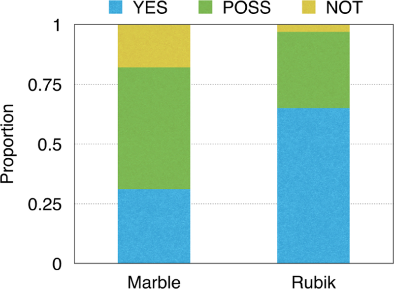
A comparison of the meaningfulness of the phenotypes discovered by Marble and Rubik.

4.2.3. Discovering Subphenotypes

Here we demonstrate how novel combinations of guidance information and pairwise constraints can lead to the discovery of fine-grained subphenotypes. In this analysis, we add the diagnosis guidance to hypertension, type 1 diabetes, type 2 diabetes and heart failure separately.

To gain an intuitive feel for how guidance works, let us use the guidance for hypertension as an example. We construct the guidance matrix ${\widehat{\mathbf{A}}}^{\left(2\right)}$ as follows. Assume the index corresponding to hypertension to be n. Then, we set the n^th entry of vector ${\widehat{\mathbf{A}}}_1^{\left(2\right)}$ and ${\widehat{\mathbf{A}}}_2^{\left(2\right)}$ to be one and all other entries equal to zero. The pairwise constraint will push ${\mathbf{A}}_1^{\left(2\right)}$ and ${\mathbf{A}}_2^{\left(2\right)}$ to be as orthogonal as possible (i.e., small cosine similarity). In other words, the resulting factors will share less common entries, and will thus be more distinct. In summary, by introducing multiple identical guidance factors (e.g., 2 hypertension vectors), the algorithm can derive different subphenotypes which fall into a broader phenotype described by the guidance factors.

Table 6 shows an example phenotype for hypertension patients that was discovered using Marble. While this phenotype may be clinically meaningful, it is possible to stratify the patients in this phenotype into more specific subgroups. Table 7 demonstrates the two subphenotypes discovered by Rubik with the hypertension guidance, which effectively include non-overlapping subsets of diseases and medications from the Marble derived phenotype.

Table 6:

An example of a Marble-derived phenotype.

Diagnoses	Medications
Chronic kidney disease	Central sympatholytics
Hypertension	Angiotensin receptor blockers
Unspecified anemias	ACE inhibitors
Fluid electrolyte imbalance	Immunosuppressants
Type 2 diabetes mellitus	Loop diuretics
Other kidney disorders	Gabapentin

Table 7:

Examples of Rubik-derived subphenotypes. The two tables show separate subgroups of hyper-tension patients: A) metabolic syndrome, and B) secondary hypertension due to renovascular disease.

A. Metabolic syndrome phenotype
Diagnoses	Medications
Hypertension	Calcineurin inhibitors
Chronic kidney disease	Insulin
Ischemic heart disease	Immunosuppressants
Disorders of lipoid metabolism	ACE inhibitors
Anemia of chronic disease	Calcium channel blockers
	Antibiotics
	Statins
	Calcium
	Cox-2 inhibitors
B. Secondary hypertension phenotype
Diagnoses	Medications
Secondary hypertension	Class V antiarrhythmics
Fluid & electrolyte imbalance	Salicylates
Unspecified anemias	Antianginal agents
Hypertension	ACE inhibitors
	Calcium channel blockers
	Immunosuppressants

In a similar fashion to the evaluation of the interaction tensor, we asked domain experts to evaluate the meaningfulness of subphenotypes. Rubik incorporated four guidance constraints (for four separate diseases), and generated two subphenotypes for each guidance constraint, resulting in eight possible subphenotypes. Domain experts were asked to evaluate whether or not each subphenotype was made sense as a subtype of the original constraint. The inter-rater agreement is 0.81. On average, the clinicians identified 62.5% (5 out of 8) of all subphenotypes as clinically meaningful, and the remaining 37.5% of subphenotypes to be possibly clinically meaningful. None of the subphenotypes were identified as not clinically meaningful. These results suggest that Rubik can be effective for discovering subphenotypes given knowledge guided constraints on the disease mode.

4.2.4. More Distinct Phenotypes

One important objective of phenotyping is to discover distinct phenotypes. In this experiment, we show that adding pairwise constraints guidance reduces the overlap between phenotypes. We also fix λ_a = 0 and change the weight of pairwise constraint (λ_q) to evaluate the sensitivity of Rubik to this constraint.

We first define cosine similarities between two vectors x and y as $cos\left(\mathbf{x},\mathbf{y}\right)=\frac{\langle \mathbf{x},\mathbf{y}\rangle }{\Vert \mathbf{x}\Vert \Vert \mathbf{y}\Vert }$. Then we use AvgOverlap to measure the degree of overlapping between all phenotype pairs. This is defined as the average of the cosine similarities between all phenotype pairs in the diagnosis mode. The formulation for AvgOverlap is as follows.

$$AvgOverlap=\frac{{\sum }_{m=1}^R{\sum }_{n>m}^{R}cos\left({\mathbf{A}}_m^{\left(2\right)},{\mathbf{A}}_n^{\left(2\right)}\right)}{R\left(R-1\right)/2}$$

where ${\mathbf{A}}_m^{\left(2\right)}$ denotes the m^th column of factor matrix A⁽²⁾, which is the vector representation of the m^th phenotype on the diagnosis mode.

Figure 2 shows the change of average cosine similarity as a function of λ_q. We can see that the average similarity tends to stabilize when λ_q is larger than 10. Figure 2 also compares Rubik with Marble, CP-APR and TF-BPP. Note that the three competitors do not incorporate pairwise constraints and clearly lead to significantly overlap in their phenotypes. As such, we can conclude that adding the pairwise constraints can effectively lead to more distinct phenotypes.

Figure 2:

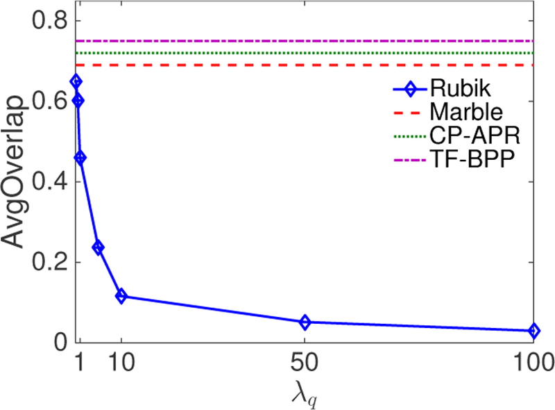
The average level of overlap in the phenotypes as a function of the pairwise constraint coefficient λ_q.

4.3. Noise Analysis

There are multiple sources of noise in real clinical applications. For example, part of the EHR data could be missing or simply incorrect. Alternatively, the clinical guidance could be noisy. To test Rubik against such conditions, we systematically evaluate different scenarios of noise. The results are summarized over 10 independent runs.

4.3.1. Robustness to Missing Data

The EHR data may have missing records. Consequentially, the observed binary tensor $\mathcal{O}$ might contain missing values. To emulate the missing data, we flip the value of each non-zero cell ${\mathcal{O}}_{\overrightarrow{i}}$ to zero with probability p.

Let $\mathcal{T}=〚{\mathbf{A}}^{\left(1\right)};\cdots ;{\mathbf{A}}^{\left(N\right)}〛$ be the solution without missing data and ${\mathcal{T}}^p=〚{\mathbf{A}}^{p\left(1\right)};\cdots ;{\mathbf{A}}^{p\left(N\right)}〛$ be the solution with missing data level p on the input tensor $\mathcal{O}$. We first pair ${\mathcal{T}}^p$ with $\mathcal{T}$ using a greedy algorithm. Then we define the average cosine similarities (AvgSim) between $\mathcal{T}$ and ${\mathcal{T}}^p$ as

$$AvgSim\left(\mathcal{T},{\mathcal{T}}^p\right)=\frac{{\sum }_{n=1}^N{\sum }_{r=1}^{R}cos\left({\mathbf{A}}_r^{\left(n\right)},{\mathbf{A}}_r^{p\left(n\right)}\right)}{NR}$$ (13)

Figure 3 shows the change in similarity measures with the change of missing-data level. It can be seen that Rubik performs well even if 30% of the data is missing, indicating its robustness. By contrast, the other baseline methods are not robust to missing data quantities as small as 10%.

Figure 3:

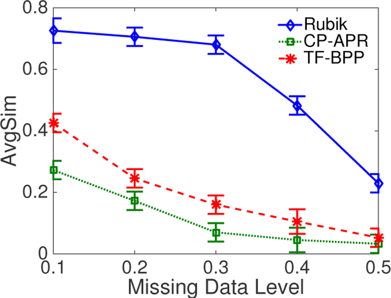
An average similarity comparison of different methods as a function of the missing data level.

4.3.2. Robustness to Noisy Data

In creating documentation in the EHR dataset, clinicians may introduce erroneous diagnosis and medication information. The implication of such errors is that the observed binary tensor $\mathcal{O}$ will also contain noise. To emulate this setting, we randomly select zero value cells, such that the total number of selected cells is equal to the number of non-zero cells. Then, for each cell in this collection, we flip its value with probability p. The difference from introducing missing data is that we introduce multiple incorrect ones as noisy data while missing data case will remove multiple correct ones.

Figure 4 shows that Rubik performs well - even when the noise level is as high as 20% – 30%. One intuitive explanation for such a high tolerance is that the model is dependent on the observed tensor, as well as various constraints. In summary, Rubik is resilient to noise. As such, Rubik will provide more generalizable phenotypes than its competitors.

Figure 4:

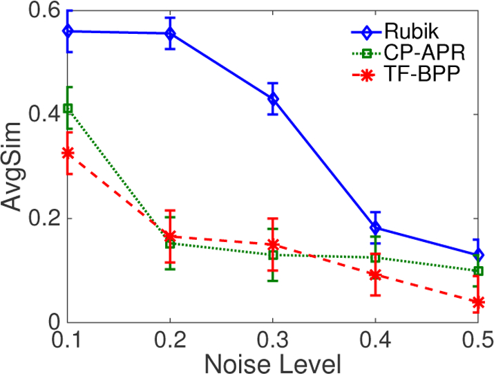
An average similarity comparison of different methods as a function of the noise level.

4.3.3. Robustness to Incorrect Guidance

At times, guidance knowledge may be incorrectly documented (or the state of medical belief may be incorrect). Take hypertension for example, to simulate incorrect guidance on this diagnosis, we randomly pick K (we use 4 in our experiments) entries from the corresponding column in the guidance matrix ${\widehat{\mathbf{A}}}^{\left(2\right)}$ and set it to be one with probability p. Note K is small here for two reasons. First, in phenotyping applications we hope to achieve sparse solutions, which implies that the guidance should also be sparse. Second, medical experts do not typically have much guidance on a particular phenotype.

We then compare the cosine similarity between the phenotypes obtained by correct and incorrect guidance. Figure 5 demonstrates that as the level of incorrect guidance increases the cosine similarity slowly decreases. Therefore, even when a significant portion of the guidance is incorrect, the phenotype can remain fairly close to the original.

Figure 5:

The similarity between the true solution and the solution under incorrect guidance as a function of the incorrect guidance level.

4.3.4. Parameter Tuning

Rubik computes the sparse factor representation using a set of predefined thresholds γ_n, which provide a tunable knob to adjust the sparsity of the candidate phenotypes. In our experiment, we numerically evaluate the sensitivity of the sparse solution with respect to different threshold values. To do so, we randomly downsample the tensor $\mathcal{O}$ by 50% and run Rubik on this smaller tensor. The above procedure is averaged over 10 independent runs.

Figure 6 shows the distribution of the non-zero factor values along the three modes. For all three plots, there is a noticeable difference in size between the first two bins, which suggests the threshold occur at the start of the second bin. Thus, for the paper, we set γ = 0.00005, 0.0001 and 0.01 for the patient, diagnosis and medication modes, respectively.

Figure 6:

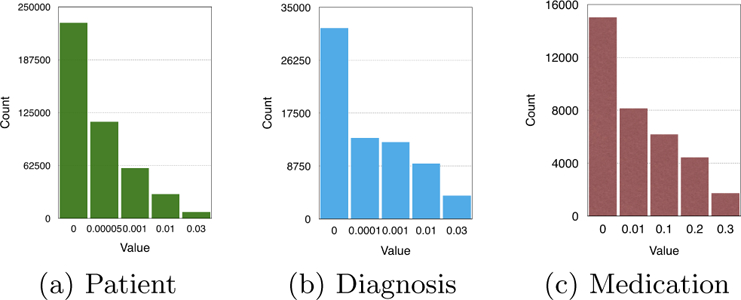
The count of non-zero elements along the three modes as a function of the thresholding parameters.

4.4. Scalability

We test the scalability of Rubik on both datasets. We randomly sample a different number of patients from the datasets and construct the tensors. The results are summarized over 10 independent runs and the performance is measured in runtime (seconds).

Figure 7 reports the runtime comparison of different tensor factorization methods on the V anderbilt dataset. We can clearly see the advantage of our framework over CP-APR. Specifically, the runtime is reduced by 70%. TF-BPP is comparable to Rubik on the V anderbilt dataset. For the CMS dataset, Rubik is around six times faster than the two baselines.

Figure 7:

A runtime comparison of different methods on the V anderbilt dataset as a function of the number of patients.

For the tensor completion task, Figure 7 shows that Rubik is nearly 5–7 times faster than WCP and FaLRTC. Figure 8 further demonstrates Rubik’s superiority over these methods. Note that FaLRTC and WCP will reach their maximum default number of iterations before the algorithm actually converges on the CMS dataset, so that more time is actually needed to complete the baselines.

Figure 8:

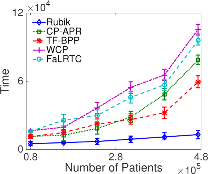
A runtime comparison of different methods on the CMS dataset as a function of the number of patients.

4.5. Constraints Analysis

We investigate the sensitivity of Rubik with regard to three constraints: completion, guidance and pairwise constraints. We begin by running Rubik under baseline conditions without any constraints. Then, we iteratively add constraints independently and compute AvgSim (Eq. 13) between the solution obtained with that constraint and without that constraint. Then, we normalize all AvgSim scores and let them sum to one. The contribution of each constraint is measured by the normalized AvgSim score. Note that we did not incorporate guidance information into Rubik on the CMS dataset.

Figure 9 reports the proportion of each constraint’s contribution to the overall model. The bars labeled Basic represent the baseline performance of the model without any constraints imposed. The bars labeled Pairwise, Guidance and Completion represent the contributions of the corresponding constraints, respectively. We see that all of the constraints represent a significant contribution to the model’s overall performance. Amongst the constraints, the pairwise constraint provides the largest contribution to the performance.

Figure 9:

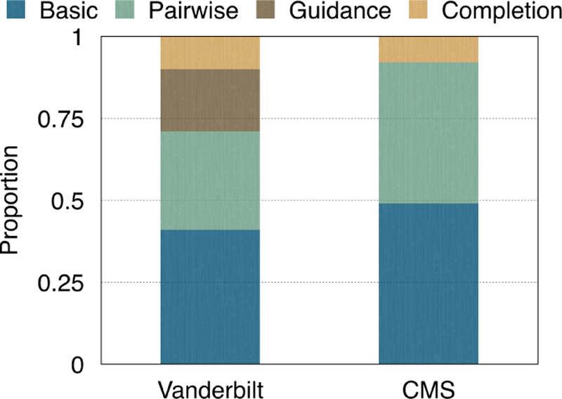
Proportion of contribution of each constraint.

5. RELATED WORK

Non-negative Tensor Factorization.

Kolda [19] provided a comprehensive overview of tensor factorization models [19]. It is desirable to impose a non-negativity constraint on tensor factorizations in order to facilitate easier interpretation when analyzing non-negative data. Existing non-negative matrix factorization algorithms can be extended to non-negative tensor factorization. Welling and Webber proposed multiplicative update algorithm [32]. Chi and Kolda [9] proposed nonnegative CP alternation Possion regression (CP-APR) model. Kim et al. [18] proposed an alternating non-negative least square method with a block pivoting technique.

Constrained Factorization.

Incorporating guidance in tensor factorization has drawn some attention over the past few years. Carroll et al. [5] used linear constraints. Davidson [10] proposed a framework to incorporate pattern constraints for network analysis of fMRI data. However, this method is domain specific and might not be applicable to other areas such as computational phenotyping. Narita [25] provided a framework to incorporate auxiliary information to improve the quality of factorization. However, this work fails to incorporate nonnegativity as constraints to the factor matrix. Solving for non-negativity constraints usually requires a nontrivial calculation step.

Coupled Factorization.

In this case, we have additional data matrices that share the same dimension as the tensor. The goal is to jointly factorizing the tensor and matrices [13]. Acar et al. [2] used first order optimization techniques. There are also scalable algorithms on Hadoop [3, 26]. However, this framework does not directly cover all the constraints we need in our application.

Tensor Completion.

Liu et al. [22] and Signoretto [29] generalized matrix completion to the tensor case to recover a low-rank tensor. They defined the nuclear norm of a tensor as a convex combination of nuclear norms of its unfolding matrices. Tomioka and Suzuki [31] proposed a latent norm regularized approach. Liu et al. [23] substituted the nuclear norm of unfolding matrices by the nuclear norm of each factor matrix of its CP decomposition. A number of other alternatives have also been discussed in [20, 24, 28]. However, these methods suffer from high computational cost of SVDs at each iteration, preventing it from scaling to large scale problems.

Without minimizing the nuclear norm, Acar et al. [1] proposed to apply tensor factorization in missing data to achieve low rank tensor completion. However, none of these methods are guaranteed to output a non-negative factor matrix for each mode or non-negative tensor. As a consequence they are not applicable to our non-negative tensor setting. Incorporating non-negativity as constraints to factor matrices, Xu et al. [33] proposed an alternating proximal gradient method for non-negative tensor completion. However, they did not take the guidance information into account and their gradient based method is not scalable to large datasets.

In summary, existing tensor factorization and completion methods are not applicable to computational phenotyping.

6. CONCLUSION

This paper presents Rubik, a novel knowledge-guided tensor factorization and completion framework to fit EHR data. The resulting phenotypes are concise, distinct, and interpretable. One distinguishing aspect of Rubik is that it is able to discover subphenotypes. Furthermore, Rubik captures the baseline characteristics of the overall population via an augmented bias tensor.

In the experiments, we demonstrate the effectiveness of adding the guidance on diagnosis. Rubik can also incorporate guidance from other sources such as medications and patients. We also demonstrate the scalability of Rubik on simulated EHRs in a dataset with millions of records. Rubik can potentially be used to rapidly characterize and manage a large number of diseases, thereby promising a novel solution that can benefit very large segments of the population. Future work will focus on evaluating Rubik on larger datasets and conduct larger medical validations with experts.