Percolation models of pathogen spillover

Abstract

Predicting pathogen spillover requires counting spillover events and aligning such counts with process-related covariates for each spillover event. How can we connect our analysis of spillover counts to simple, mechanistic models of pathogens jumping from reservoir hosts to recipient hosts? We illustrate how the pathways to pathogen spillover can be represented as a directed graph connecting reservoir hosts and recipient hosts and the number of spillover events modelled as a percolation of infectious units along that graph. Percolation models of pathogen spillover formalize popular intuition and management concepts for pathogen spillover, such as the inextricably multilevel nature of cross-species transmission, the impact of covariance between processes such as pathogen shedding and human susceptibility on spillover risk, and the assumptions under which the effect of a management intervention targeting one process, such as persistence of vectors, will translate to an equal effect on the overall spillover risk. Percolation models also link statistical analysis of spillover event datasets with a mechanistic model of spillover. Linear models, one might construct for process-specific parameters, such as the log-rate of shedding from one of several alternative reservoirs, yield a nonlinear model of the log-rate of spillover. The resulting nonlinearity is approximately piecewise linear with major impacts on statistical inferences of the importance of process-specific covariates such as vector density. We recommend that statistical analysis of spillover datasets use piecewise linear models, such as generalized additive models, regression clustering or ensembles of linear models, to capture the piecewise linearity expected from percolation models. We discuss the implications of our findings for predictions of spillover risk beyond the range of observed covariates, a major challenge of forecasting spillover risk in the Anthropocene.

This article is part of the theme issue ‘Dynamic and integrative approaches to understanding pathogen spillover’.

1. Introduction

Pathogen spillover is a critical process in the emergence of infectious diseases [1], and its prediction may facilitate the preemption of zoonotic outbreaks [2]. Pathogen spillover itself occurs as a result of a series of events, from pathogen shedding and persistence to human contact and infection of a human host [3]. Yet, outstanding questions remain regarding how to best predict spillover risk, determine the relative importance of these various spillover processes and connect mechanistic models with statistical analysis of spillover data.

Spillover prediction accuracy depends on both our understanding of the underlying process and its parameters, and on the spatio-temporal and phylogenetic scales at which the prediction is made [4–6]. For example, Childs et al. [7] curated a dataset of yellow fever incidence over a near-continental spatial scale (the country of Brazil), pooling counts of yellow fever incidence within municipalities for each municipality-month over 16 years. The phylogenetic scale of their data—the lineage of organisms over which predictions were made—was defined by any incident determined to be ‘yellow fever’, thus pooling strain-level variation. The authors also used a phylogenetic scale of ‘primates’ as reservoirs when calculating the estimates of environmental risk. Their model, a boosted regression tree, estimated the probability of spillover occurring within that municipality. The probability of spillover was assumed to depend on process-related covariates such as human vaccine coverage, human population densities and environmental risk (several variables constructed to reflect the propensity of bites from infected mosquitoes), among others.

Most empirical efforts to predict pathogen spillover will probably mirror the steps of Childs et al. and require observations of spillover defined over spatial, temporal and phylogenetic scales. Spillover observations are tabulated as counts of the number of spillover events (within the appropriate scales of space, time and phylogeny or taxonomy). The counts are then aligned with process covariates that are believed to be relevant for those scales, such as temperature, reservoir density and human susceptibility. The goals of compiling and analysing such data are typically twofold: (i) to understand the relative importance of various processes, from reservoir shedding to human susceptibility, in the observed variation in spillover, and (ii) to forecast spillover for the sake of management prioritization or preemption. Incorporating projected changes in reservoir densities, vector densities and environmental covariates into spillover predictions will often require extending forecasts beyond previously observed conditions, as these covariates will probably respond to the changing climate, land use and other human pressures in the Anthropocene. To forecast beyond the range of contemporary observations, we need tractable mechanistic models of spillover which connect with the inferential machinery used to forecast pathogen spillover risk.

Spillover occurs when pathogens find some path from animal reservoirs to susceptible human hosts. These pathways to spillover—the inclusive series of events between shedding and detection of an infected human as discussed in Plowright et al. [3]—can be represented as a directed graph along which infectious units move from animals to people. The infectious units produced through shedding or vector contact of infected reservoirs progress through these stages toward spillover and suffer attrition as fractions die owing to a failure to persist in the environment, contact humans, infect humans given contact and be detected as a spillover event in our dataset. From these first principles of pathogen spillover, we construct a family of probabilistic models of the percolation of pathogens from a reservoir host to a recipient host. We refer to these models as ‘percolation models of pathogen spillover.’

Percolation models are commonly used to describe the movement of infection through a contact network [8]. Here, however, we use ‘percolation model’ in the strict mathematical sense, as the stochastic movement of material along a graph [9]. Instead of the movement of infections along a contact network, we consider the movement of infectious units along the stages that link reservoir hosts to reported infections in humans (or other recipient host of interest, such as cattle acquiring Brucellosis). Representing pathogen spillover through percolation models yields a family of simple, stochastic models connecting the assumed mechanisms of spillover to the count data typically analysed to estimate spillover risk.

In the first part of this paper, we outline percolation models that correspond to different assumptions about the pathway(s) of pathogen spillover. We develop conceptual tools useful for discussing spillover risk and assigning relative importance to various steps of the spillover process. We show that log-probabilities are a natural way to analyse percolation processes and yield simple statistically rooted concepts for management, such as the amount of risk managed by a proposed countermeasure. Under some percolation models of pathogen spillover, such as pathogens spilling over from multiple reservoirs or pathogens taking alternative pathways from reservoirs to recipient hosts, the log-probabilities yield nonlinearities that provide insight into potential pitfalls of statistical inferences of spillover risk and its associations with covariates, especially when projecting outside the range of observed covariates.

In the second part of this paper, we study parameter estimation in percolation models of spillover. We show that the rate parameters of pathogen spillover implied by percolation models are often nonlinear functions of canonical parameters used for inference in generalized linear models (GLMs) [10]. We show that if the log-odds of attrition probabilities are linear functions of covariates, or if the log-rates of shedding from alternative reservoirs are linear functions of covariates, the resulting nonlinear log-rates of spillover will be approximately piecewise linear. We show that statistical tools capable of modelling piecewise linear functions, such as piecewise cubic splines in generalized additive models or ensembles of linear models, perform reasonably well at capturing the nonlinearities produced by percolation models of spillover.

Throughout this paper, we highlight that percolation models allow researchers to connect their inferences with a first-principles model of pathogen spillover and we formalize the fundamental challenges and limitations in analyses of spillover datasets. Percolation models of spillover provide some traction into analysis through the tractable behaviour of filtered and pooled Poisson or negative binomial counts of infectious units, new avenues for visualizing spillover model structures and concepts and intuition of value for managers attempting to control the inextricably multilevel process of pathogen spillover. We show how inescapable nonlinearities arising from percolation models affect and how spillover will respond to changing environmental conditions—such as which reservoir may become the dominant reservoir or which attrition processes could become rate limiting outside the observed range of environmental conditions or under a new management action. Percolation models are not the final solution to modelling the spillover process but are proposed as a rigorous mathematical and statistical framework to bridge an identified gap in the field [3,5,6]. There are some restrictive assumptions in percolation models as presented here, such as the independent progression of infectious units from the same source and the assumption that infectious units do not replicate along the pathway to spillover; these assumptions can limit the use of percolation models to various important systems. Further work can help clarify the specific pathogens and scenarios for which percolation models are and are not appropriate, and there is a need for concrete case studies to implement—and assess the value of—the mathematical and statistical framework developed here. Scripts for the simulation and analysis conducted in this paper can be found at https://github.com/reptalex/PercolationSpillover.

2. The graph structure of pathogen spillover

A series of logical events must occur for a pathogen to spillover from a reservoir host to a recipient host, though the exact series of events varies depending on the wildlife and pathogen life histories. The passage of an infectious unit through that series of events from a reservoir host to a recipient host can be represented with a model of percolation along a graph. In this paper, we consider an integer number, X, of infectious units released from the reservoir and surviving a series of logical events leading to spillover events. The pathway along which infectious units percolate from wildlife to people can be illustrated with a graph. For example, the graph below, read from left to right,

represents X infectious units produced from the reservoir. The pathway to pathogen spillover is partitioned into a series of n logical events with probabilities p₁, p₂, …, p_n of occurring. At the end of the graph, we denote a total number of spillover events, Y; spillover only occurs when a pathogen successfully overcomes each of the n barriers. Such a graph could be used to represent a percolation model of Nipah virus contacting a human through date palm sap consumption [11]. We refer to this as the ‘serial’ model for pathogen spillover.

The structure of the graph representing the pathway to spillover depends on pathogen life history. A simple modification of the graph can represent the pathway to spillover for pathogens that can follow several alternative transmission routes. For example, Ebolavirus can spillover directly from bats to people through bushmeat hunting [12], but spillover appears more likely to occur through contact with the infected carcass of an amplifier host such as a forest antelope or non-human primate [13]. If an amplifier rarely or never infects more than one person, the percolation model for Ebolavirus will have the graph structure

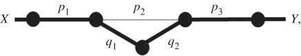
where the thick lines illustrate the most common pathway, and the route passing through the amplifier has two new probabilities: q₁, the probability an infectious unit infects an amplifier host, and q₂, the probability an infected amplifier contacts a human with an infectious dose. If amplifiers can contact more than one host, the infectious units are no longer percolating along the graph but instead replicate and branch to produce multiple spillover events. We discuss the biological scenarios which complicate the results uncovered in this paper; such complications may be fruitful avenues of future research. The percolation models we investigate are summarized in table 1.

Table 1.

Percolation-based models of pathogen spillover allow graphical visualizations of model structure (the graphs) and a clear connection between a multilevel model and resulting probabilities of percolation and rates of spillover. (Here, λ_i is the rate of shedding from source i, p_j is the probability of surviving level j, p_i,j the probability of surviving level j along pathway i and ${\mathbb{I}}_i$ is the indicator function equal to 1 if the pathogen is shed from source i and 0 otherwise. Percolation models can be easily adapted for different pathogens with different pathways to spillover, and most adaptations yield similar nonlinearities whose impacts on spillover rates and statistical inference we discuss in this paper.) (Online version in colour.)

model	graph	probability of percolation, PS	rate of spillover, ${\mathit{\lambda }}_{\mathbf{S}}$	example
serial		$\prod _{\hspace{0.17em}j=1}^n{p}_j$	$\lambda \prod _{\hspace{0.17em}j=1}^n{p}_j$	Ebolavirus, Marburgvirus
detour		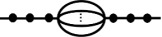$\left(\prod _{\hspace{0.17em}j\ne l}^n{p}_j\right)\left(\sum _{i=1}^m{\alpha }_i{p}_{i,l}\right)$	$\lambda \left(\prod _{\hspace{0.17em}j\ne l}^n{p}_j\right)\left(\sum _{i=1}^m{\alpha }_i{p}_{i,l}\right)$	Bartonella spp.
alt. sources		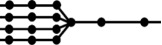$\left({\mathbb{I}}_i\prod _{\hspace{0.17em}j\le l}{p}_{i,j}\right)\left(\prod _{k>l}{p}_k\right)$	$\left(\sum _i{\lambda }_i\prod _{\hspace{0.17em}j\le l}{p}_{i,j}\right)\left(\prod _{k>l}{p}_k\right)$	Giardia lamblia
time lag (step l)		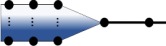$\left({\int }_0^{\mathrm{\infty }}{\mathbb{I}}_{\tau }\left(\prod _{i=1}^{l-1}{p}_j(t-\tau )\right)p_l(t,\hspace{0.17em}\tau )h(\tau )\hspace{0.17em}\mathrm{d}\tau \right)\times \left(\prod _{k>l}{p}_k\right)$	$\left({\int }_0^{\mathrm{\infty }}\lambda (t-\tau )\left(\prod _{i=1}^{l-1}{p}_j(t-\tau )\right)p_l(t,\hspace{0.17em}\tau )h(\tau )\hspace{0.17em}\mathrm{d}\tau \right)\times \left(\prod _{k>l}{p}_k\right)$	Nipah virus

For notation, we will always use X as the random variable representing the number of infectious units shed or released from the reservoir and P_S—the probability of spillover—will denote the probability that an individual infectious unit infects a human or other recipient host. We use p to denote probabilities for logical events on the pathway to pathogen spillover, with single subscripts (p_j) representing the jth event and dual subscripts (p_i,j) representing the ith alternative pathway for the jth event. Finally, Y will represent a filtered number of infectious units after a series of logical events, with Y_j representing the number of infectious units surviving j events. In general, the subscript j will denote event j in a series of events to pathogen spillover, i will indicate an alternative pathway, and l will be reserved for a focal intermediate node or measurement pool in the pathway to spillover.

(a) Serial—conceptualization of percolation

Passage of infectious units through the graph can be modelled with a series of Bernoulli random variables, B_j, where the probability that an infectious unit passes the jth barrier occurs with a ‘success’ probability of p_j (figure 1). The random variable $B_{\mathrm{S}}={\prod }_j{B}_j$ indicates whether an infectious unit makes it through every barrier to eventually infect a person. In this serial model of a single pathway to pathogen spillover, the probability a given infectious particle causes a human infection is

$$\begin{array}{c}{P}_{\mathrm{S}}=\prod _{\hspace{0.17em}j=1}^n{p}_j.\end{array}$$ 2.1

Figure 1.

Partitioning the pathway to spillover into a series of logical events allows one to model, study, conceptualize and visualize risk maps of spillover across levels. Percolation models subdivide spillover into a series of events, such as environmental persistence or viral replication, in-between which there are pools of potential observations, such as the number of human exposures or the number of infected humans. Some variation in the overall risk of pathogen spillover can be explained through known associations between log-probabilities log(p_j) of each event j in the series and external covariates. A management action can differentially impact the probabilities of each event happening leading to a degree of manageable risk under a proposed intervention. Covariances between attrition rates at different levels, and even directionality of changes following a management action, can be visualized with asymmetric graphs of manageable risk. Pathogen spillover is an inextricably multilevel process. As such, quantifying the manageable risk requires knowing the impacts of management actions on every one of the series of events separating a wildlife pathogen from a human infection. Unknown or unstudied levels can impact the overall effect of an intervention on spillover risk. Such unknown effects must be explicitly recognized and can be either assumed to be unaffected or prioritized for further study.

Percolation processes yield some traction into analysis of count processes frequently used to model infectious particle release or spillover events. If we assume the number of virions released into the environment is a Poisson random variable, $X\sim \mathrm{Pois}(\lambda )$, and a serial percolation process filters viruses—each virion having probability p_j of surviving step j on the pathway to spillover—then the number of spillover events is

$$\begin{array}{c}\begin{array}{c}\begin{array}{c}Y\sim \mathrm{Binom}(X,\hspace{0.17em}{P}_{\mathrm{S}}),\end{array}\end{array}\end{array}$$ 2.2

which is easily shown to follow a Poisson distribution, $Y\sim \mathrm{Pois}(P_{\mathrm{S}}\lambda ).$ Similarly, if $X\sim \mathrm{NegBinom}(\mu ,\hspace{0.17em}\psi )$, then $Y\sim \mathrm{NegBinom}(P_{\mathrm{S}}\mu ,\hspace{0.17em}\psi )$ (see the electronic supplementary material for proofs). In both the Poisson and the negative binomial cases, the emergent number of spillover events is a filtered version of the original random variable as the starting counts have been ‘filtered’ through the series of Bernoulli trials represented by the graph up until the pool of interest. The fact that filtered Poisson and negative Binomial count distributions retain their distributional form through the percolation model is a useful feature for analysis and statistical inference as it connects shedding rates and survival probabilities to the end result of a random number of spillover events.

Equation (2.1) indicates the importance of log-scale changes in the probability of success at various stages. For example, all else being equal, if changing the ambient temperature halves the probability a virion survives long enough to contact a human but doubles the probability of infection given contact owing to temperature-dependent changes in human susceptibility, the risk of pathogen spillover will remain unchanged [14–16]. More generally, by analysing the variance of the log-probability of spillover, one can partition variance in spillover risk into ‘explained variance’ and ‘manageable variance’. Explained variance is the total amount of variance in spillover risk we can explain with existing models, and manageable variance is the fraction of explained variance in spillover risk one can modify with management interventions such as ecological interventions [17] (figure 1; see the electronic supplementary material for proof). The effects of a changing covariate or implemented management action, compared with a control scenario of no change or no management action, can be illustrated by showing the potentially competing effects at multiple levels on the pathway to spillover. The final impact of such an action can be estimated using equation (2.1) with explicit acknowledgement of the levels about which there is fundamental uncertainty or lack of knowledge on the explained or manageable variance (figure 1). These concepts, and the resulting intuition, are formalized by analysis of the spillover risk and its variance under a serial model of percolation (electronic supplementary material).

(b) Alternative pathways/detours

In many cases, the assumption of a single pathway to pathogen spillover is unrealistic. Pathogens such as Bartonella spp. or avian influenza virus could be transmitted by one of many transmission routes [18–20]. In these scenarios, the graphical model becomes

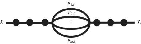
where level l has m alternative pathways (in the case of Bartonella spp. or avian influenza virus, alternative transmission routes) and p_i,l is the probability of a pathogen surviving the ith alternative pathway given entry to that pathway. If α_i is the fraction of infectious units in the pool prior to l which go down the ith alternative pathway such that $\sum _i{\alpha }_i=1$, then the probability a given infectious unit spills over becomes

$$\begin{array}{c}\begin{array}{c}\begin{array}{c}{P}_{\mathrm{S}}=\left(\prod _{\hspace{0.17em}j\ne l}^n{p}_j\right){⟨{\mathit{p}}_l⟩}_{\mathit{\alpha }},\end{array}\end{array}\end{array}$$ 2.3

where ${⟨{\mathit{p}}_l⟩}_{\mathit{\alpha }}={\sum }_i{\alpha }_i{p}_{i,l}$ is the weighted average probability of surviving level l.

Taking the logarithm of both sides of equation (2.3), we encounter a nonlinearity through the logarithm of an arithmetic mean:

$$\begin{array}{c}\begin{array}{c}\begin{array}{c}\log P_{\mathrm{S}}=\log \left(\sum _{i=1}^m{\alpha }_i{p}_{i,l}\right)+\sum _{\hspace{0.17em}j\ne i}^n\log (\hspace{0.17em}{p}_j).\end{array}\end{array}\end{array}$$ 2.4

This log-sum nonlinearity affects our ability to make neat inferences on the impact of doubling or halving the probabilities of success along one of the alternative pathways. Similarly, the variance of a log-sum cannot be easily expressed in terms of variances and covariances of each log-probability. However, as we show in the electronic supplementary material, the nonlinearity of equation (2.4) can be understood, and we show that it results in the final spillover counts closely resembling the counts along the pathway with the highest rate of successful percolations, which we refer to as the ‘dominant pathway’. The effect of pathway dominance on our statistical inferences with spillover count datasets is discussed later.

(c) Alternative sources

Many pathogens can spillover from one of the multiple reservoirs. Examples of pathogens spilling over from multiple animal reservoirs include Yersinia pestis [21], Escherichia coli [22], Giardia lamblia [23], Borrelia burgdorferi [24] and more. For m alternative reservoirs whose shed or vector-borne pathogens follow independent pathways until a common pool at level l, the percolation graph becomes

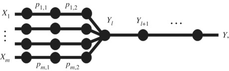
where X_i is the amount of pathogen released from reservoir i, p_i,j is the probability that the pathogen released from reservoir i successfully passes level j, and Y_l is the amount of pathogen pooled at step l, after l logical events. We will use l to denote the first point at which pathogens from different reservoirs enter a common pool, such as avian influenza virions arriving into a common pond after being shed by multiple waterfowl hosts [25,26] or yellow fever virions from alternative primate reservoirs and vectors arriving in a common pool of exposed humans (e.g. as considered in Childs et al. [7]).

Prior to pooling, each pathway has a separate, serial percolation model with the usual results: a Poisson shedding random variable for species i, $X_i\sim \mathrm{Pois}({\lambda }_i)$ yields a filtered Poisson random variable prior to pooling, $Y_{i,l-1}\sim \mathrm{Pois}({\lambda }_i{\prod }_{\hspace{0.17em}j<l}\hspace{0.17em}{p}_{i,j}).$ As we have shown in the electronic supplementary material, a similar result holds for negative binomial counts.

At the intersecting node of the pathways from alternative sources, the separate Poisson or negative binomial random variables arising from each reservoir host species are added to yield the number of infectious units in the common pool. For the Poisson case, since the sum of Poisson random variables is also Poisson, with a rate equal to the sum of the contributing rates, the number of infectious units surviving up to the common pool will be

$$\begin{array}{c}\begin{array}{c}\begin{array}{c}{Y}_l\sim \mathrm{Pois}\left(\sum _i{\lambda }_i\prod _{\hspace{0.17em}j\le l}{p}_{i,j}\right).\end{array}\end{array}\end{array}$$ 2.5

The expected number of spillover events can be calculated by recognizing that percolation is a serial between Y_l and Y (table 1). Negative binomial random variables with different means can be pooled to yield a negative binomial random variable if and only if their dispersion parameters are equal. Because binomial filtration of negative binomial counts only affects the mean and not the dispersion, results analogous to equation (2.5) hold if one assumes the negative binomial dispersion parameters are equal across alternative sources. Otherwise, one could construct a negative binomial approximation of pooled negative binomial counts (e.g. with a negative binomial random variable whose mean and variance is equal to that of the pool), the accuracy and validity of which will depend on the downstream questions.

Pooling comes from a variety of processes. In addition to pooling of pathogens from multiple reservoirs in datasets where we cannot tell which reservoir is responsible for a spillover event, researchers often pool infections within some phylogenetic scale that defines a species or strain or disease category under study—e.g. one study may separate Lyme disease incidents from rocky mountain spotted fever incidents as they are caused by distinct bacterial species, whereas another may pool the two as tick-borne bacterial diseases. Such questions of the phylogenetic scale of our predictions [5,6] define our data and how we pool counts. If researchers are interested in potential strain-specific rates of pathogen shedding, survival in the environment or other events, but are unable to distinguish between strains in a spillover dataset, their data will be generated by a count process like that of equation (2.5). As we show in the section on statistical inference, pooling, a perhaps inevitable operation in our dataset construction, can introduce nonlinearities in both Poisson and negative binomial count models that complicate inference and analysis of spillover datasets.

(d) Time-dependence—percolation processes

In the previously discussed percolation models of pathogen spillover, we have implicitly assumed that both the process generating the initial pulse of infectious units from the reservoir, and the various filtrations of that pulse along the percolation graph, are instantaneous. Often, however, shedding is a time-dependent process, and our data consist of a cross-sectional sample of infectious units accumulated at a given layer at a specific point in time. In addition to shedding, the survival probabilities of infectious units may depend on temporal attributes like seasonality or time since deposition [27].

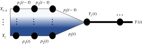
Let λ(t) be the rate of pathogen shedding at time t. Consider the time-dependence of environmental persistence combined with a variable time, τ, between shedding and recipient host exposure. For pathogen spillover to occur, pathogens shed into the environment must survive until contacting a recipient host. The environmental pool at time t, Y_l(t), will contain pathogens shed at various times in the past that have survived up to time t. Let τ be a random variable with density h(τ), p_l(t, τ) be the probability of a pathogen surviving in the environmental pool from time t − τ to t, and assume that all previous logical events are instantaneous but with time-dependent probabilities, p_j(t). Then, $Y_l(t)\sim \mathrm{Pois}({\lambda }_l(t))$, where

$$\begin{array}{c}\begin{array}{c}\begin{array}{c}{\lambda }_l(t)={\int }_0^{\mathrm{\infty }}\lambda (t-\tau )\left(\prod _{i=1}^{l-1}{p}_j(t-\tau )\right)p_l(t,\hspace{0.17em}\tau )h(\tau )\hspace{0.17em}\mathrm{d}\tau \end{array}.\end{array}\end{array}$$ 2.6

The rate defined in equation (2.6) is similar to the model of alternative sources in equation (2.6) with appropriately shifted time-dependent probabilities. Hence, nonstationary probabilities of passage and random time intervals for lagged passage through a particular level produce a temporally explicit percolation model of alternative sources for all steps including and prior to the lagged step, as illustrated below, where darker shading is used to indicate more recent shedding times:

.

The mathematical similarity between pathogen spillover from percolation models of alternative reservoirs and alternative sources in time may prove useful for researchers linking models of pathogen dynamics in reservoir hosts with a percolation model for spillover from reservoir to a new host, as the results from alternative reservoirs can help one understand how alternative sources in time are contributing to pathogen spillover.

3. Statistical inference

One aim in the analysis of spillover datasets is to estimate the relative importance of various levels or processes in the pathway to spillover. To do this, researchers compile data on the incidence of pathogen spillover and covariates believed to be related by some statistical model to the rates of shedding or the probabilities that infectious units progress onwards through various processes on the pathway to spillover [28–30]. Barring data on intermediate pools of pathogens Y_j, one may hope to quantify the relative importance of each level through the curation of a dataset with level-specific covariates, z_j, hypothesized to explain some variation in the probability of spillover for level j. For example, in an alternative source model, one may measure the reservoir population densities of all alternative sources in the locales where spillover occurred. Typically, large-scale studies of spillover work with a set of pooled counts of spillover events, Y, representing successful infections at the end of the percolation model of spillover, and use regression to determine spillover risk and assess the relative importance of different covariates and barriers to spillover.

Percolation models for spillover illuminate two challenges for such statistical inferences using pooled counts. The challenges arise from the difference between the probability and rate parameters used in the derivation of equations (2.1)–(2.6), and the canonical parameters—logit probabilities and log-rates—used for GLMs of exponential family random variables. While the probability and rate parameters combine nicely for tractable mathematical analyses of percolation models, statistical inference through GLMs estimate canonical parameters obtained by evaluating nonlinear link functions of the probability or rate parameters. The nonlinearity of link functions for the Poisson, negative binomial and Bernoulli random variables present in the percolation models of spillover has important consequences for interpreting results from a regression on Y and the inference of the relative importance of various steps and pathways to spillover. In this section, we will denote canonical parameters η(z) as functions of a single covariate z, and the random variable for that covariate will be Z. While few studies aim to predict spillover with a single covariate and linear models (e.g. Childs et al. [7] use an ensemble of boosted regression trees to predict spillover counts), we focus on one covariate for simplicity and aim to understand nonlinearities and their challenges for inference through the comprehensible perspective of a GLM. We expect systems with multiple covariates to exhibit qualitatively similar behaviour and illustrate how even nonlinear modelling approaches can fail in light of percolation-induced nonlinearities.

(a) Serial

The simplest percolation model of pathogen spillover for statistical inference will contain a pathogen pulse, such as $X\sim \mathrm{Pois}(\lambda (z))$, and the probability of spillover, P_S(z), combined to yield a filtered distribution for the number of spillover events, such as $Y\sim \mathrm{Pois}(P_{\mathrm{S}}(z)\lambda (z))$ for the Poisson case. In a GLM framework, whether one assumes a Poisson or negative binomial model for the pathogen pulse, one typically models the canonical parameters of the two processes. For both Poisson and negative binomial models of pathogen pulses, the canonical parameters are the logarithm of the mean, λ, and thus a GLM of the counts of infectious units shed from reservoir hosts is

$$\begin{array}{rl}{\eta }_X=& \hspace{0.17em}\log (\lambda )\\ =& \hspace{0.17em}{\beta }_{X,0}+{\beta }_{X,1}z.\end{array}$$ 3.1

Similarly, for a GLM of a binomial filtration, one would typically model the log-odds of the probability an infectious unit survives filtration yielding the linear model

$$\begin{array}{rl}{\eta }_p=& \hspace{0.17em}\log \left(\frac{\hspace{0.17em}p}{1-p}\right)\\ =& \hspace{0.17em}{\beta }_{P,0}+{\beta }_{P,1}z.\end{array}$$ 3.2

However, a GLM for spillover events, Y, would estimate η_Y, the log of the rate for Y. Using the rate of Y defined by the percolation process, combined with equations (3.1) and (3.2), we see that a GLM predicting Y would model

$$\begin{array}{rl}{\eta }_Y=& \hspace{0.17em}\log (\lambda (z))+\log (\hspace{0.17em}p(z))\\ =& \hspace{0.17em}{\eta }_X-\log (1+e^{-{\eta }_p}).\end{array}$$ 3.3

Substitution with equations (3.2) and (3.3) yields

$$\begin{array}{c}\begin{array}{c}\begin{array}{c}{\eta }_Y={\beta }_{X,0}+{\beta }_{X,1}z-\log (1+e^{-{\beta }_{P,0}-{\beta }_{P,1}z}).\end{array}\end{array}\end{array}$$ 3.4

If attrition is high, defined here as 0 < p ≪ 0.5, then η_p is a negative number and the approximation $\log (1+e^{-{\eta }_P})\approx -{\eta }_P$ permits approximate superposition of intercepts and slopes for an overall linear model, yielding

$$\begin{array}{c}\begin{array}{c}\begin{array}{c}{\eta }_Y\approx ({\beta }_{X,0}+{\beta }_{P,0})+({\beta }_{X,1}+{\beta }_{P,1})z.\end{array}\end{array}\end{array}$$ 3.5

However, if attrition is low, i.e. 1 > p ≫ 0.5, then η_p is positive and the approximation $\log (1+e^{-{\eta }_P})\approx e^{-{\eta }_P}$ produces terms that are nonlinear in z_j, but if ${\beta }_{X,0}\gg e^{-{\beta }_{\hspace{0.17em}p,0}}$, the intercept and slope from shedding dominate and equation (3.6) is approximately

$$\begin{array}{c}\begin{array}{c}\begin{array}{c}{\eta }_Y\approx {\beta }_{X,0}+{\beta }_{X,1}z.\end{array}\end{array}\end{array}$$ 3.6

Thus, the appropriate linear approximation switches near η_p = 0 (P_S(z) = 0.5); this is further illustrated in figure 2.

Figure 2.

The nonlinearities of equation (3.4) affect our inferences from spillover count datasets. Simulating data under the linear model of equation (3.4) illustrates how the intercept ${\hat{\beta }}_0$ (a) and slope ${\hat{\beta }}_1$ (b) of spillover counts estimated under a generalized linear model switch between those predicted from the linear models in equations (3.3) and (3.6). For lower attrition, simulated here as a large, positive baseline log-odds of survival through percolation β_p,0, the slope of the attrition process contributes less to the observed slope of spillover counts. Thus, spillover count datasets can lead one to underestimate the potential sensitivity of a level to management action well outside the range of observed covariates. (c) These results stem from the approximate piecewise linearity of the canonical parameter one can calculate from a percolation model of pathogen spillover. Here, we plot the nonlinearity of the canonical parameter as a function of the covariate, z, across a range of intercepts for the baseline log-odds of an infectious unit surviving the percolation along the pathway to spillover.

The nonlinearity of canonical parameters as functions of rate and probability parameters in percolation processes yields important intuition and general rules for statistical inference of the association between covariates and the number of spillover events. First, linear models of the log-odds of success in a serial percolation model generate nonlinear models in the log-rate of spillover. However, that nonlinearity is not intractable. Equations (3.5) and (3.6) reveal that if attrition probabilities are rarely close to 0.5, these nonlinear models are approximately piecewise linear. The intercepts and slopes of the log-rate of shedding and log-odds of attrition are added to produce the intercepts and slopes for the overall spillover rate only for attrition processes with high attrition. For processes with low attrition, the associations between attrition and covariates can be lost, even for sensitive processes with strong associations (high β_P,1) whose change in log-odds of success may be consequential for management. One may assume a GLM for each level or a GLM for the number of spillover events, but not both, unless the log-odds of success for each level remain high or remain low. More generally, if one assumes linearity at each level, the log-rate of spillover should be examined for piecewise linearity and the possible masking of sensitive yet low-attrition processes (figure 2).

(b) Alternative pathways and sources

Statistical inference for alternative pathways and sources is analysed in the electronic supplementary material. Our analysis provides insight into how linear or piecewise constant models of spillover risk can err, especially when projecting beyond the observed range of covariates. In addition, as mentioned above, GLMs of pooled counts of spillover events across alternative sources will produce regression coefficients reflecting those of the dominant pathway (figure 3). If a pathway is highly sensitive—i.e. has a large slope with respect to some covariate—but non-dominant owing to a low intercept and comparatively low variance of the covariate with a high slope, it will be very difficult to identify as a highly manageable or sensitive pathway in a spillover count dataset.

Figure 3.

Pooled counts of infectious units from alternative pathways produce a nonlinearity similar to the nonlinearity arising from attrition. In this manuscript, we show this common nonlinearity inherent in percolation models of spillover is approximately a switching or piecewise linearity. If one reservoir or source is the dominant source in our dataset (a) but another, more sensitive source (b) could become dominant outside the range of observed covariates owing to its association with a covariate, z, the pooled counts will not follow a generalized linear model (GLM) (c,d). If pathway switching—the exchange of dominance across alternative pathways—is observed (c), then percolation models reveal how piecewise linear [34] or piecewise cubic splines such as those in generalized additive models (GAMs) can produce accurate predictions outside the range of observed covariates. If pathway switching is not observed (d), then, like the low-attrition processes in figure 2, the sensitivity of non-dominant pathways can be invisible to the machinery we use to infer how spillover risk will change with the covariate.

While one should always look for heteroskedasticity to ensure a model is a good fit, our results suggest it is especially important to check for switching dominance and piecewise linearity when predicting pathogen spillover risk from alternative sources in space, time or species, as such piecewise or switching linearity is to be expected from the first-principles model proposed and analysed here. Where dominance switching occurs within a dataset and monotonically along a covariate or direction for multiple covariates, piecewise linear models—such as piecewise cubic splines for generalized additive models or ensembles of linear models—can capture the true effects and predict well beyond the observed range of covariates. Regression clustering or switching-regression models [31,32] may separate data points with different dominant pathways for datasets in which pathway switching does not occur along any direction in the observed covariates. If dominance switching is possible but unobserved, due to hypersensitive pathways which are not dominant in our dataset, hypersensitive yet non-dominant sources will be extremely hard to detect. A default statistical analysis of spillover count datasets which fails to consider the nonlinearities arising under a percolation model is prone to miss potentially useful inferences of sensitive alternative pathways, as spillover counts will tend to reflect the behaviour of the dominant pathway.

4. Conclusion

Pathogen spillover is a stochastic, multilevel process whose prediction can determine the value of surveillance, the effectiveness of countermeasures and the changing landscape of spillover risk in a changing world [3]. Here, we developed stochastic, multilevel percolation-based models of pathogen spillover. Percolation models of pathogen spillover can be visualized with graphs indicating the pathways to spillover, and various percolation models can be analysed to yield clear connections between model structure, data analysis and management paradigms for inferring and mitigating spillover risk.

For a serial percolation model, one can decompose the variance in spillover risk in terms of variances and covariances of log-probabilities of each level, providing a simple and intuitive multilevel model of pathogen spillover. The decomposition of variance in spillover risk may be of use for those developing statistical and mathematical methods to model and infer spillover risk, as well as managers or meta-analysts attempting to combine piecemeal results of different processes (e.g. shedding, persistence and susceptibility) estimated across the literature. The serial percolation model of pathogen spillover produces some conceptual tools, illustrated in figure 1, towards a management paradigm to discuss known and unknown manageability of spillover. With more time and effort, this simple model of spillover may be able to interface directly with costs of interventions and allow researchers to discuss, quantitatively, the information gain of data from different levels through increased explained variance in log-probabilities of success (e.g. the value of wildlife surveillance versus vaccine coverage).

Percolation models of spillover lend themselves to easy visualizations of model structure and tractable calculations of spillover rates. They also provide two important results for the inference of spillover risk across levels and across alternative pathways. In general, one cannot use GLMs for both levels or alternative sources and the overall rate of spillover. However, when one assumes linear models between a covariate and the log-rates of shedding from alternative sources and/or the log-odds of successful passage through a barrier to spillover, the resulting nonlinearity is always approximately piecewise linear. Thus, count data of spillover incidence should be carefully analysed for piecewise linearity using tools such as generalized additive models, switching-regression models or ensembles of linear models. Projections beyond the range of observed covariates should be especially wary of the piecewise linearity arising in the log-rate of pathogen spillover. The switching dominance and invisibility of processes with weak attrition, even if they have a strong sensitivity to management actions, present a unique challenge for pathogen spillover data analysis and management. If two studies are conducted in two areas with different dominant reservoirs having different associations with a management action, they may obtain contradictory results. Only by understanding the mechanisms by which alternative sources and attrition processes are associated with covariates and management actions can we hope for generality.

Percolation models do not yet yield a recipe for the analysis of spillover count datasets. Rather, researchers will have to consider various phenomena described here on a case-by-case basis owing to the wide range of data quality, data quantity, research questions and underlying biology in pathogen spillover datasets. The usual statistical concerns of model complexity; which covariates to include, the behaviour of regularization, how to quantify the relative importance of covariates and so on, must be considered in light of the behaviour of spillover counts we have shown here. For example, lasso regression [33] could easily shrink the slope for a covariate to zero when the slope is in fact high but invisible owing to its modulation of a non-dominant source or a currently low-attrition process on the pathway to spillover. More generally, based on the results in figures 2 and 3, we suspect such approaches, which are typically employed to prevent overfitting, could exacerbate the challenges of identifying sensitive yet non-dominant pathways and weak attrition processes. At the current stage, we see these percolation models not as a general recipe for statistics as much as a tool for understanding—and in some cases using clever experimental design, data collection or statistical analyses to avoid—the pitfalls facing data analysts and managers in the field. If our work suggests one firm recommendation to analysts of spillover count datasets, it is that the assumption that spillover counts can be neatly analysed with standard GLMs of covariates collected to correspond to alternative reservoirs or processes on the pathway to spillover is an extremely tenuous assumption. Furthermore, we show the ways—pathway switching and attrition probabilities going from low to high—in which nonlinearities arise and estimates of the relative importance of alternative pathways and processes one obtains from GLMs can be consequentially wrong.

Percolation models are a simple model and a useful approximation of pathogen spillover, allowing one to statistically decompose the wildlife-human contact rates into a series of measurable processes which may have different associations with covariates or responses to management actions. However, percolation models will fail to be useful approximations when some assumptions do not hold. When infectious particle replication in intermediate pools is non-negligible, such as replication within alternative pathways reliably leading to one virion causing potentially multiple infections, we cannot model spillover as simply the attrition of shed infectious units. Similarly, percolation models do not capture the epidemiological feedbacks that may exist between environmental or vector pools and wildlife reservoir hosts. Finally, where dose–response filters are crucial, one can play with the definition of an ‘infectious unit’, but the spatial distribution and non-independence of such infectious units may be relevant and capturing such detail may require additional model complexity not captured by percolation models.

Percolation models arise from first principles of pathogen spillover from reservoirs to recipient hosts and allow a tuneable level of complexity for modelling spillover risk ranging from a coin toss—spillover happens with probability P_S—to a fully deterministic system in which alternative sources and pathways are determined with probability 1. Percolation models can be a modular component for models of spillover risk; one could model shedding as an externally defined stochastic process, as we have assumed here, or one could model shedding through more commonly employed susceptible-resistant-exposed (SIR)-type epidemiological models. Regardless of the model of shedding, if cycles and replication along the pathway to spillover is negligible, percolation models serve as a module connecting shedding to an end result of spillover counts. Even deterministic models of shedding can be input for percolation models of spillover. Bayesian efforts to obtain posterior probabilities of various models and their parametrizations can also be connected with percolation models, as a posterior distribution over different model structures can be incorporated through a stochastic sampling of different models’ shedding trajectories over time or space.

All models are wrong, but the percolation models we propose may provide useful intuition and results for conceptualizing, managing, analysing and forecasting the risk of pathogen spillover. Percolation models are not the final solution to modelling the spillover process but are proposed as a rigorous mathematical and statistical framework to address an identified gap in the field [3,5,6]. Further work can help clarify the specific pathogens and scenarios for which percolation models are and are not appropriate, and there is a need for concrete case studies to implement—and assess the value of—the mathematical and statistical framework developed here.

Data accessibility

Scripts for the simulation and analysis conducted in this paper can be found at https://github.com/reptalex/PercolationSpillover.

Authors' contributions

A.D.W. conceived, analysed and simulated percolation models and was the main author of the paper. D.E.C., K.R.M, D.J.B. and M.L.C assisted with analysis of percolation models, connections with biological literature and the writing of the MS. R.K.P. assisted with the conception, analysis and integration with biological literature and contributed to the writing of the manuscript.

Competing interests

We declare we have no competing interests.

Funding

We received no funding for this study.

References

- 1.Power AG, Mitchell CE. 2004. Pathogen spillover in disease epidemics. Am. Nat. 164, S79–S89. ( 10.1086/424610) [DOI] [PubMed] [Google Scholar]
- 2.Morse SS, Mazet JAK, Woolhouse M, Parrish CR, Carroll D, Karesh WB, Zambrana-Torrelio C, Lipkin WI, Daszak P. 2012. Prediction and prevention of the next pandemic zoonosis. Lancet 380, 1956–1965. ( 10.1016/S0140-6736(12)61684-5) [DOI] [PMC free article] [PubMed] [Google Scholar]
- 3.Plowright RK, Parrish CR, McCallum H, Hudson PJ, Ko AI, Graham AL, Lloyd-Smith JO. 2017. Pathways to zoonotic spillover. Nat. Rev. Microbiol. 15, 502 ( 10.1038/nrmicro.2017.45) [DOI] [PMC free article] [PubMed] [Google Scholar]
- 4.Washburne AD, Silverman JD, Morton JT, Becker DJ, Crowley D, Mukherjee S, David LA, Plowright RK. 2019. Phylofactorization: a graph partitioning algorithm to identify phylogenetic scales of ecological data. Ecol. Monogr. 89, e01353 ( 10.1002/ecm.1353) [DOI] [Google Scholar]
- 5.Becker DJ, Washburne AD, Faust CL, Pulliam JRC, Mordecai EA, Lloyd-Smith JO, Plowright RK. 2019. Dynamic and integrative approaches to understanding pathogen spillover. Phil. Trans. R. Soc. B 374, 20190014 ( 10.1098/rstb.2019.0014) [DOI] [PMC free article] [PubMed] [Google Scholar]
- 6.Becker DJ, Washburne AD, Faust CL, Mordecai EA, Plowright RK. 2019. The problem of scale in the prediction and management of pathogen spillover. Phil. Trans. R. Soc. B 374, 20190224 ( 10.1098/rstb.2019.0224) [DOI] [PMC free article] [PubMed] [Google Scholar]
- 7.Childs ML, Nova N, Colvin J, Mordecai EA. 2019. Mosquito and primate ecology predict human risk of yellow fever virus spillover in Brazil. Phil. Trans. R. Soc. B 374, 20180335 ( 10.1098/rstb.2018.0335) [DOI] [PMC free article] [PubMed] [Google Scholar]
- 8.Keeling MJ, Eames KTD. 2005. Networks and epidemic models. J. R. Soc. Interface 2, 295–307. ( 10.1098/rsif.2005.0051) [DOI] [PMC free article] [PubMed] [Google Scholar]
- 9.Stauffer D, Aharony A. 2014. Introduction to percolation theory: revised, 2nd edn Boca Raton, FL: CRC Press. [Google Scholar]
- 10.Nelder JA, Wedderburn RWM. 1972. Generalized linear models. J. R. Stat. Soc. Ser. A 135, 370–384. ( 10.2307/2344614) [DOI] [Google Scholar]
- 11.Rahman MA, et al. 2012. Date palm sap linked to Nipah virus outbreak in Bangladesh, 2008. Vector-Borne Zoonotic Dis. 12, 65–72. ( 10.1089/vbz.2011.0656) [DOI] [PubMed] [Google Scholar]
- 12.Leroy EM, Epelboin A, Mondonge V, Pourrut X, Gonzalez J-P, Muyembe-Tamfum J-J, Formenty P. 2009. Human Ebola outbreak resulting from direct exposure to fruit bats in Luebo, Democratic Republic of Congo, 2007. Vector-Borne Zoonotic Dis. 9, 723–728. ( 10.1089/vbz.2008.0167) [DOI] [PubMed] [Google Scholar]
- 13.Pourrut X, Kumulungui B, Wittmann T, Moussavou G, Délicat A, Yaba P, Nkoghe D, Gonzalez J-P, Leroy EM. 2005. The natural history of Ebola virus in Africa. Microbes Infect. 7, 1005–1014. ( 10.1016/j.micinf.2005.04.006) [DOI] [PubMed] [Google Scholar]
- 14.Stallknecht DE, Kearney MT, Shane SM, Zwank PJ. 1990. Effects of pH, temperature, and salinity on persistence of avian influenza viruses in water. Avian Dis. 34, 412–418. ( 10.2307/1591429) [DOI] [PubMed] [Google Scholar]
- 15.Lowen AC, Mubareka S, Steel J, Palese P. 2007. Influenza virus transmission is dependent on relative humidity and temperature. PLoS Pathog. 3, e151 ( 10.1371/journal.ppat.0030151) [DOI] [PMC free article] [PubMed] [Google Scholar]
- 16.Lowen AC, Steel J. 2014. Roles of humidity and temperature in shaping influenza seasonality. J. Virol. 88, 7692–7695. ( 10.1128/JVI.03544-13) [DOI] [PMC free article] [PubMed] [Google Scholar]
- 17.Sokolow SH. et al. 2019. Ecological interventions to prevent and manage zoonotic pathogen spillover. Phil. Trans. R. Soc. B 374, 20180342 ( 10.1098/rstb.2018.0342) [DOI] [PMC free article] [PubMed] [Google Scholar]
- 18.Pepin KM, Hopken MW, Shriner SA, Spackman E, Abdo Z, Parrish C, Riley S, Lloyd-Smith JO, Piaggio AJ. 2019. Improving risk assessment of the emergence of novel influenza A viruses by incorporating environmental surveillance. Phil. Trans. R. Soc. B 374, 20180346 ( 10.1098/rstb.2018.0346) [DOI] [PMC free article] [PubMed] [Google Scholar]
- 19.Breitschwerdt EB, Kordick DL. 2000. Bartonella infection in animals: carriership, reservoir potential, pathogenicity, and zoonotic potential for human infection. Clin. Microbiol. Rev. 13, 428–438. ( 10.1128/CMR.13.3.428) [DOI] [PMC free article] [PubMed] [Google Scholar]
- 20.Becker DJ, Bergner LM, Bentz AB, Orton RJ, Altizer S, Streicker DG. 2018. Genetic diversity, infection prevalence, and possible transmission routes of Bartonella spp. in vampire bats. PLoS Negl. Trop. Dis. 12, e0006786 ( 10.1371/journal.pntd.0006786) [DOI] [PMC free article] [PubMed] [Google Scholar]
- 21.Butler T. 2012. Plague and other Yersinia infections. Berlin, Germany: Springer Science & Business Media. [Google Scholar]
- 22.Ferens WA, Hovde CJ. 2011. Escherichia coli O157: H7: animal reservoir and sources of human infection. Foodborne Pathog. Dis. 8, 465–487. ( 10.1089/fpd.2010.0673) [DOI] [PMC free article] [PubMed] [Google Scholar]
- 23.Appelbee AJ, Thompson RCA, Olson ME. 2005. Giardia and Cryptosporidium in mammalian wildlife–current status and future needs. Trends Parasitol. 21, 370–376. ( 10.1016/j.pt.2005.06.004) [DOI] [PMC free article] [PubMed] [Google Scholar]
- 24.Mather TN, Wilson ML, Moore SI, Ribeiro JM, Spielman A. 1989. Comparing the relative potential of rodents as reservoirs of the Lyme disease spirochete (Borrelia burgdorferi). Am. J. Epidemiol. 130, 143–150. ( 10.1093/oxfordjournals.aje.a115306) [DOI] [PubMed] [Google Scholar]
- 25.Webster RG, Yakhno M, Hinshaw VS, Bean WJ, Murti KC. 1978. Intestinal influenza: replication and characterization of influenza viruses in ducks. Virology 84, 268–278. ( 10.1016/0042-6822(78)90247-7) [DOI] [PMC free article] [PubMed] [Google Scholar]
- 26.Breban R, Drake JM, Stallknecht DE, Rohani P. 2009. The role of environmental transmission in recurrent avian influenza epidemics. PLoS Comput. Biol. 5, e1000346 ( 10.1371/journal.pcbi.1000346) [DOI] [PMC free article] [PubMed] [Google Scholar]
- 27.Martin G, Becker DJ, Plowright RK. 2018. Environmental persistence of influenza H5N1 is driven by temperature and salinity: insights from a Bayesian meta-analysis. Front. Ecol. Evol. 6, 131 ( 10.3389/fevo.2018.00131) [DOI] [Google Scholar]
- 28.Rogers DJ, Randolph SE, Snow RW, Hay SI. 2002. Satellite imagery in the study and forecast of malaria. Nature 415, 710 ( 10.1038/415710a) [DOI] [PMC free article] [PubMed] [Google Scholar]
- 29.Pigott DM, et al. 2014. Mapping the zoonotic niche of Ebola virus disease in Africa. Elife 3, e04395. [DOI] [PMC free article] [PubMed] [Google Scholar]
- 30.Brierley L, Vonhof MJ, Olival KJ, Daszak P, Jones KE. 2016. Quantifying global drivers of zoonotic bat viruses: a process-based perspective. Am. Nat. 187, E53–E64. ( 10.1086/684391) [DOI] [PMC free article] [PubMed] [Google Scholar]
- 31.Hathaway RJ, Bezdek JC. 1993. Switching regression models and fuzzy clustering. IEEE Trans. Fuzzy Syst. 1, 195–204. ( 10.1109/91.236552) [DOI] [Google Scholar]
- 32.Lokshin M, Sajaia Z. 2004. Maximum likelihood estimation of endogenous switching regression models. Stata J. 4, 282–289. ( 10.1177/1536867X0400400306) [DOI] [Google Scholar]
- 33.Tibshirani R. 1996. Regression shrinkage and selection via the lasso. J. R. Stat. Soc. Series B 58, 267–288. ( 10.1111/j.2517-6161.1996.tb02080.x) [DOI] [Google Scholar]
- 34.Muggeo VMR, et al. 2008. Segmented: an R package to fit regression models with broken-line relationships. R News 8, 20–25. [Google Scholar]
Associated Data
This section collects any data citations, data availability statements, or supplementary materials included in this article.
Supplementary Materials
Data Availability Statement