Visual recency bias is explained by a mixture model of internal representations

Abstract

Human bias towards more recent events is a common and well-studied phenomenon. Recent studies in visual perception have shown that this recency bias persists even when past events contain no information about the future. Reasons for this suboptimal behaviour are not well understood and the internal model that leads people to exhibit recency bias is unknown. Here we use a well-known orientation estimation task to frame the human recency bias in terms of incremental Bayesian inference. We show that the only Bayesian model capable of explaining the recency bias relies on a weighted mixture of past states. Furthermore, we suggest that this mixture model is a consequence of participants’ failure to infer a model for data in visual short term memory, and reflects the nature of the internal representations used in the task.

Introduction

In a rapidly changing world our model of the environment needs to be continuously updated. Often recent information is a better predictor of the environment than the more distant past (Anderson & Milson, 1989; Anderson & Schooler, 1991): for example, the location of a moving object is better predicted by its location one second ago than a minute ago. However, human observers seem to rely on recent experience even when it provides no information about the future at all (Fischer & Whitney, 2014; Cicchini, Anobile, & Burr, 2014; Burr & Cicchini, 2014; Fritsche, Mostert, & de Lange, 2017; Liberman, Fischer, & Whitney, 2014). Such recency bias seems to be domain-general and not constrained to a particular task or feature dimension (Kiyonaga, Scimeca, Bliss, & Whitney, 2017). Why should this be so, and what can it tell us about the mechanisms of perception and memory?

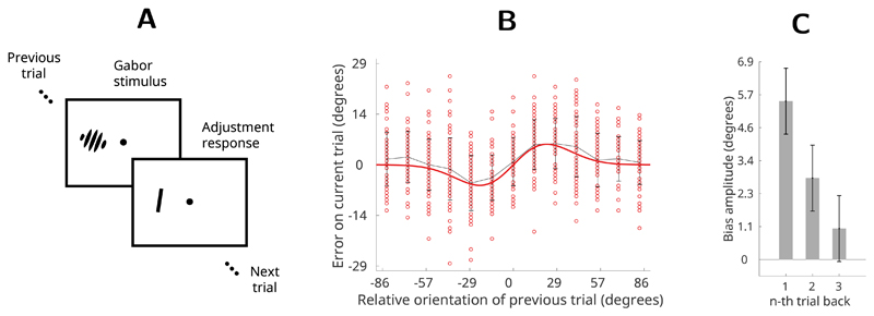
The most extensive quantitative data on the human recency bias comes from a study of visual orientation estimation by Fischer and Whitney (2014). In that study participants were presented with a randomly oriented grating (Gabor) on each trial and asked to report the orientation by adjusting a bar using the arrow keys (Fig 1A).

Figure 1. Orientation estimation task (Fischer & Whitney, 2014).

(A) Participants observed randomly oriented Gabor stimuli and reported the orientation of each Gabor by adjusting a response bar. Stimuli were presented for 500 ms and separated in time by 5s. (B) Single subject’s errors (red dots) as a function of the relative orientation of the previous trial. Gray line is average error; red line shows a first derivative of a Gaussian (DoG) curve fit to the data. (C) Average recency bias amplitude across participants computed for stimuli presented one, two and three trials back from the present. Error bars represent ±1 standard deviation of the bootstrapped distribution.

Participants’ error distributions revealed that although responses were centred on the correct orientations over the course of the entire experiment, on a trial-by-trial basis the reported orientation was systematically (and precisely) biased in the direction of the orientation seen on the previous trial. For example, when the Gabor on the previous trial was oriented more clockwise than the Gabor on the present trial, participants perceived the present Gabor as being tilted more clockwise than its true orientation (Fig 1B).

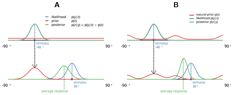
Since the orientations of the stimuli were generated randomly in this task the recency bias indicates that participants are not behaving optimally. In other words, the previous trial contained no information about the next trial and hence the optimal model would consider all orientations as equally likely in the future. In this case the participants’ error distributions would simply be proportional to the sensory noise and always centred around the true stimulus value (Fig 2A, top row). However, here participants assume a model of the environment where past states are informative about the future (Fig 2A, bottom row), which is clearly false.

Figure 2. Bayesian orientation estimation and recency bias.

Participant’s estimate of the orientation (p(z|y), green line) combines sensory evidence (p(y|z), blue line) with prior expectation (p(z), red line). Participant’s response can be thought of as a sample from the posterior distribution. All distributions are Von Mises since orientation is a circular variable. (A) Top row: for optimal behaviour participant’s prior should be flat and posterior equal to the sensory evidence. Bottom row: Recency bias occurs when information about previous stimuli (orientation estimate at trial n−1, green line in top row) is transferred to the prior expectation about the next stimulus (red line, bottom row). Here the prior for trial t is just the posterior from previous trial t − 1. (B) Natural prior model. Top row: participants prior is based on the statistics of the natural environment (Girshick et al., 2011). Bottom row: participants prior is a mixture of the previous stimulus and the natural statistics.

In the current study we use the orientation estimation task (Fischer & Whitney, 2014) to investigate what is the participants’ model of the environment that gives rise to the recency bias. We frame this question in terms of sequential Bayesian inference which allows us to test hypotheses about the participant’s model of the environment at any trial given sensory information (orientation of the Gabor) and the recorded response (Fig 2, see also Bayesian orientation estimation in Supporting Information). We test three alternative hypotheses about the model behind the recency bias which are all formulated as sequential Bayesian inference models so that they can be directly compared to each other.

Von Mises filter

First, we test the hypothesis that participants assume that the current state of the environment is the best guess about it’s future. This identity model is the simplest Bayesian incremental updating model (a Bayesian filter) that can plausibly represent the orientation estimation task. Bayesian filters (such as the Kalman filter, Kalman & Bucy, 1961) are widely used in explaining human behaviour and have been previously proposed to explain the temporal continuity effects in perception (Burr & Cicchini, 2014; Wolpert & Ghahramani, 2000; Rao, 1999).

Here we use the circular approximation of the Kalman filter called the Von Mises filter (VMF) where the latent state and measurement noise are distributed according to Von Mises and not Gaussian distributions (Kurz, Gilitschenski, & Hanebeck, 2016; Marković & Petrović, 2009). An example of a simple VMF is depicted on Fig 2A, where the prediction p(z_t) at the bottom row is derived from the previously estimated posterior distribution p(z_t1 |y_t−1), or in other words, the latent state transition model is identity. See Von Mises filter in Methods for details.

Natural prior model

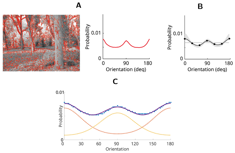
A simple identity model as outlined above ignores the fact that people’s orientation judgements are more accurate at cardinal orientations, reflecting the statistics of contours in natural environment (Girshick et al., 2011). Such bias suggests that the observer’s internal model matches the environment, a hallmark of Bayesian optimality. Fig 3 depicts orientation statistics of a natural image and participants’ orientation sensitivity extracted from a behavioural task (Girshick et al., 2011). Hence we can supplement the identity model with a natural prior so that participants modulate the identity prediction by taking into account the natural statistics of orientations in the environment.

Figure 3. Natural prior for orientation (Girshick et al., 2011).

(A) A natural image (left) and a distribution of contour orientations extracted from the image. (B) Average prior distribution of orientations across all participants estimated with a noisy orientation judgement task. The grey error region shows ±1 standard deviation of 1,000 bootstrapped estimated priors. (C) Observers’ average prior as reported by Girshick et al., 2011 (dotted blue line) represented as a mixture of two Von Mises distributions (solid blue line), which has two components peaking at cardinal orientations (dotted yellow and red lines).

Since the size of the recency bias in the task was independent of stimulus orientation (Fischer & Whitney, 2014) we can rule out a static natural prior in advance. Instead, we assume here that the prior is a mixture of the stimulus on the previous trial and the natural prior distribution. An illustration of a single step in the natural prior model is depicted on Fig 2B, where the prediction z_t is equal to the mixture of the previous stimulus and a static natural prior. See Natural prior model in Methods for details.

Mixture model

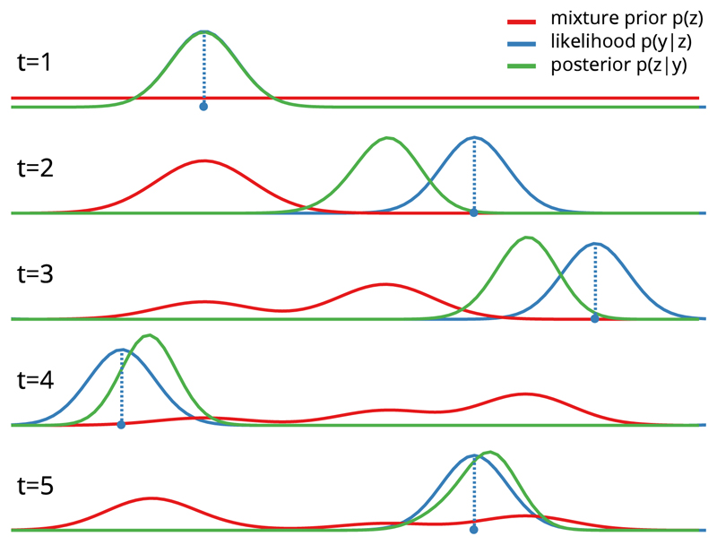
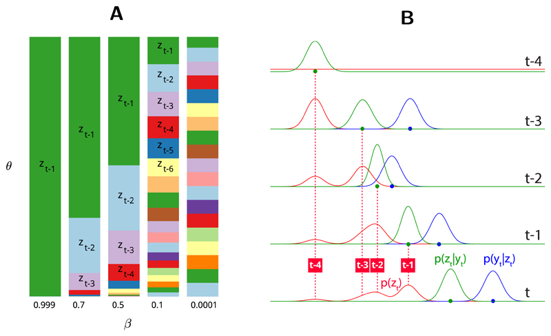
Last, we test the hypothesis that participants’ predictions incorporate information from multiple past trials. Such a mixture model assumes that the participant’s model of the environment is a mixture of multiple past states so that more recent states contribute more than older ones. The two previous hypotheses both assume that the model of the environment p(z) is inferred only based on the previous latent state. Contrastingly, the human recency bias clearly extends beyond the previous state – it is greatest for the most recent state and decays for each further state into the past (Fig 1C). In order to model such time-decaying recency bias over several past states we modify the VMF so that its prior distribution reflects a time-decaying mixture of information from multiple previous trials. Fig 4 illustrates the evolution of the latent state p(z) in a mixture model over 4 trials. Importantly, such mixture distribution is computed by a fixed sampling step (Kalm, 2017) which results in a computationally first-order Markovian model which has the same number of parameters and model complexity as the natural prior model described above. See Mixture model in Methods for details.

Figure 4. Mixture model.

Evolution of the mixture latent state over five trials.

Note that we can a priori rule out approaches which track the average orientation or some other summary statistic (Hubert-Wallander & Boynton, 2015; Dubé, Zhou, Kahana, & Sekuler, 2014) since with random stimuli they would all be uninformative about the past (however, see Manassi, Liberman, Chaney, & Whitney, 2017 for sequential dependencies in summary statistical judgments themselves).

Methods

Von Mises filter

Here we use the circular approximation of the Kalman filter called the Von Mises filter (VMF) where the latent state and measurement noise are distributed according to Von Mises and not Gaussian distributions,

$$z_t=a\left(z_{t-1}\right)+q_t{q}_t\sim VM\left(0,{\kappa }_{Q_t}\right)$$ (1)

$$y_t=h\left(z_t\right)+r_t{r}_t\sim VM\left(0,{\kappa }_{L_t}\right)$$ (2)

where κ_Q and κ_L are latent state and measurement noise concentration terms respectively. An example of a simple VMF is depicted on Fig 2B, where both state transition and measurement models are identity functions and state noise is zero, resulting in a model where the predicted state z_t is equal to the previously estimated posterior distribution p(z_t1 |y_t−1). The posterior distribution, being a product of two Von Mises distributions and representing participant’s estimate, therefore also approximates Von Mises (see Product of two von Mises distributions in Supporting Information for details):

$$p\left(z_t|y_t\right)\propto VM\left({\mu }_{E_t},{\kappa }_{E_t}\right).$$ (3)

This allows us to define recency bias on any trial t as the distance which posterior mean μ_Et has moved away from the presented stimulus y_t towards some previous stimulus value y_t−n. Such estimation error represents the systematic shift in participants’ responses since the internal estimate of the perceived orientation (Eq 3) is not centred around the presented stimulus y_t (Fig 2). The value of the estimation error, as a distance between the posterior mean and stimulus value, can be easily derived from the properties of Von Mises product:

$$y_t-{\mu }_{E_t}=\text{arctan}\frac{{\kappa }_{Q_t}\text{sin}\left(y_t\right)}{{\kappa }_{Q_t}\text{cos}\left(y_t\right)+{\kappa }_{L_t}}$$ (4)

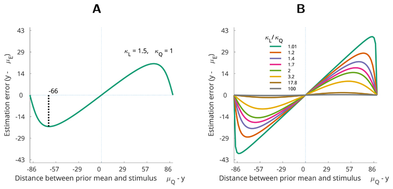
Importantly, this estimation error function (Eq 4) allows us to describe the possible space of recency biases by mapping the systematic shift of the estimation error towards previously observed orientations (Fig 5).

Figure 5. Recency bias with Von Mises distributions.

(A) Example of Von Mises recency bias with fixed prior and likelihood parameters (κ_L = 1.5, κ_Q = 1, Eq 4). Recency bias is greatest when the distance between the prior mean and stimulus (x-axis) is ca 66 degrees (1.15 radians) (black dotted line). (B) The shape of the recency bias depends on the ratio of likelihood to prior concentration κ_Lt/κ_Qt (differently coloured lines). See Von Mises filter properties in Supporting Information for details.

Such mapping of all possible shapes of the recency bias (Fig 5B) reveals that when Von Mises distributions are used for Bayesian inference the recency bias always peaks more than halfway through the x-axis (Fig 5, for a proof, see Von Mises filter properties in Supporting Information). This property means that the VMF cannot even theoretically yield a DoG-like recency bias shape as observed with human participants (Fig 1B).

Model parameters

To model the perceptual noise around the stimulus value (Eq 2) we used a fixed concentration parameter for the likelihood function (κ_L), which was chosen so as to produce the just noticeable difference (JND) values matching human data from Fischer and Whitney (2014) (average JND was 5.39°, hence σ = 3.8113° and κ_L = 0.0688). The concentration parameter for the state noise κ_Q was a free parameter optimised to minimise the distance between the simulated data and the average observed subjects’ response (see Model fitting and parameter optimisation in Supporting Information).

Natural prior model

We modified the VMF so that instead of predicting the next state based on the current one (identity model) we assume that everything else being equal, cardinal orientations are more likely than oblique ones and reflect this in our prediction. We can do this by using the natural prior distribution function as the state transition model which changes the predictive prior distribution p(z_t|z_t−1) on trial t from unimodal Von Mises to bimodal non-parametric distribution. For this purpose we model the average observers’ prior as reported by Girshick et al. (2011) as a mixture of two Von Mises probability distributions, which has two components peaking at cardinal orientations (solid blue line on Fig 3C):

$$a\left(z\right)\sim {\beta }_{1}VM\left(z;0,{\kappa }_1\right)+{\beta }_{2}VM\left(z;\pi ,{\kappa }_2\right)=\frac{\text{exp}\left({\kappa }_1\text{cos}\left(\text{z}\right)\right)}{2\pi I_0\left({\kappa }_1\right)}+\frac{\text{exp}\left({\kappa }_2\text{cos}\left(z-\pi \right)\right)}{2\pi I_0\left({\kappa }_2\right)}$$ (5)

We can now specify the equations for the Bayesian filter (Eq 1,2) with the natural prior with a state transition model a(z_t−1) is a bimodal mixture peaking at cardinal orientations (Eq 5, Fig 3C), the measurement model is identity, and the noise for both is additive Von Mises.

However, if the prior would always predict cardinals over obliques, we would only observe recency bias for the trials which were preceded by orientations close to cardinal angles. Since the size of the recency bias in the behavioural experiment was independent of stimulus orientation (Fischer & Whitney, 2014) we can rule out a fixed natural prior (Eq 5) in advance. Instead, we assume here that the prior is a mixture of the natural prior and the previous posterior.

$$a\left(z_{t-1}\right)\sim \stackrel{previousposterior}{\overbrace{{\beta }_{1}p\left(z_{t-1}|y_{t-1}\right)}}+\stackrel{naturalprior}{\overbrace{{\beta }_{2}VM\left(z;0,{\kappa }_1\right)+{\beta }_{3}VM\left(z;\pi ,{\kappa }_2\right)}}$$ (6)

This leads to a prediction which is still biased towards the previous trial but mixed with the natural prior (Fig 6). In general terms, we assume here that participants have both a bias towards previous orientations and natural statistics of the environment (Fig 3). Importantly, such multi-modal prior means that participants estimates (posterior distribution) are also not Von Mises which allows for recency bias curves qualitatively different from Von Mises ones.

Figure 6. Prior distribution as a mixture between the previous posterior p(z_t−1|y_t−1) and the natural prior distribution (Eq 5).

Depicted are two mixtures of the same components. (A) Equal mixture (solid blue line) of 50% previous posterior (dotted red line) and 50% natural prior (dotted green line). (B) Mixture (solid blue line) of 10% previous posterior (dotted red line) and 90% natural prior (dotted green line).

Model parameters

For the natural prior model (NPM) we used the same perceptual noise parameter (κ_L) as in the VMF described above. Here we used an additional free parameter – the proportion of the previous posterior (β₁) in the prior distribution (Eq 6). Importantly, when β₁ > 0.5 (Fig 6A) the previous posterior would dominate the resulting prior and hence the model would start to approximate the VMF. Similarly, as β₁ approaches zero (Fig 6B) the natural prior component will dominate the prior distribution. As in our previous simulations we chose the free parameter values (κ_Q, β₁) to minimise the distance between the simulation and behavioural results observed by Fischer and Whitney (2014) (see Model fitting and parameter optimisation in Supporting Information for details).

Since the predictive prior distribution resulting from the mixture components is non-parametric we used a discrete circular filter to approximate the distributions in this simulation. The discrete filter is based on a grid of weighted Dirac components equally distributed along the circle (Kurz et al., 2016; Kurz, Gilitschenski, & Hanebeck, 2013) and was implemented with libDirectional toolbox for Matlab (Kurz, Gilitschenski, Pfaff, & Drude, 2015). Because in the unidimensional circular state space of orientations the quality of approximation is only given by the number of components, we felt that 10,000 Dirac components can adequately approximate a distribution of a circular variable. For details on the implementation of the filter algorithms see Discrete circular filter with Dirac components in Supporting Information.

Mixture model

In order to model a time-decaying recency bias over several past states we modify the basic VMF so that the state transition model (a(·), Eq 1) predicts the next state based on a recency-weighted mixture of m past states:

$$a\left(z_{t-1},\dots ,z_{t-m}\right)\sim {\theta }_{1}p\left(z_t|z_{t-1}\right)+\cdots +{\theta }_{m}p\left(z_t|z_{t-m}\right)={\displaystyle \sum _{m=1}^M{\theta }_{m}p\left(z_t|z_{t-m}\right).}$$ (7)

Here θ_m is a mixing coefficient for the m-th past state. We can control the individual contribution of a past state z_m to the resulting mixture distribution by defining how the mixing coefficient θ decays over the past states:

$${\theta }_m=\alpha {\theta }_0{\left(1-\beta \right)}^m.$$ (8)

Here β is the rate of decrease of the mixing coefficient over the past m states and α is a normalising constant. As a result we have a decaying time window into the past m states defined by the rate parameter β. The role of the β parameter is to control the decrease of the mixing coefficient θ over past states. Fig 7A illustrates the relationship between the β and θ parameters: the bigger the β the faster the contribution of past states decreases and greater the proportion of most recent states to the mixture distribution (Eq 7). As β approaches 1, the mixture begins to resemble z_t−1 and approximate the first-order VMF described above:

$$\underset{\beta \to 1}{\text{lim}},p\left(z_t|z_{t-1},\dots ,z_{t-m}\right)\sim p\left(z_t|z_{t-1}\right).$$ (9)

Figure 7. Mixture model.

(A) Values of the mixing coefficient θ over past states (z_t−1, . . . , z_t−m) based on different β values. θ represents the proportion of a past state z_t in the mixture distribution (Eq 7). (B) Evolution of the latent state p(z) over 4 trials.

Conversely, as β approaches zero, all past states contribute equally to the mixture. Intuitively, β could be interpreted as the bias towards more recent states. Fig 7B illustrates the evolution of the latent state distribution p(z) when β = 0.5 and the mixing coefficient decays over the previous states.

Importantly, the mixture distribution is computed by a fixed sampling step (for details of the mixture sampling algorithm see Kalm, 2017, and Mixture model in Supporting Information). Hence the mixture model is computationally first-order Markovian and has the same number of parameters and model complexity as the NPM described above.

In sum, we have a circular Bayesian filter where the state transition model a(·) is a mixture function over past m states (Eq 7). The proportion of the individual past states in the mixture – and therefore the effective extent of the window into the past – is controlled by the β parameter. As in previous models, the measurement model is identity, and both state and measurement noise (κ_Q and κ_L) are additive Von Mises.

Model parameters

We used the same perceptual noise parameter (κ_L) as in the VMF and NPM simulations described above. The free parameters in the mixture model (MM) were the mixing coefficient hyper-parameter β (Eq 8) and state noise (κ_Q). As with previous simulations, the free parameters were chosen to minimise the distance between the simulated data and the average observed subjects’ response (see Model fitting and parameter optimisation in Supporting Information).

Statistical effects of interest

In each trial, we simulated the participant’s response k_t by taking a random sample from the posterior distribution: k_t ~ p(z_t|y_t). We then calculated three statistical effects as follows:

• (1)Distribution of errors – we fit a Von Mises distribution to the simulated errors yielding mean (μ) and concentration values (κ_E). We then calculated the similarity between our simulated error distribution and participants average distribution by assessing the probability of simulated μ and κ_E given the distribution of participants bootstrapped $\overline{\mu }\text{and}\overline{{\kappa }_E}.$
• (2)DoG recency bias curve – we fit the simulated errors with a first derivative of a Gaussian curve (DoG, see Recency bias amplitude as measured by fitting the derivative of Gaussian in Supporting Information for details), and as above, calculated the probability of the curve parameters arising from the distribution of participants’ bootstrapped parameter distributions.
• (3)DoG recency bias over past three trials – we calculated the amplitude of the DoG curve peak for stimuli presented one, two and three trials back. We sought to replicate a positive but decaying recency bias over three previous stimuli.

Results

We used all three models to simulate participants’ responses using the stimuli and experimental structure provided by the authors (824 trials with fully randomised stimuli). We sought to replicate three statistical effects observed in the behavioural experiments: zero-mean distribution of the errors, DoG-like fit of the recency bias (Fig 1B), and significant recency bias over multiple past trials (Fig 1C). See Statistical effects of interest in Methods for details.

Von Mises Filter (VMF)

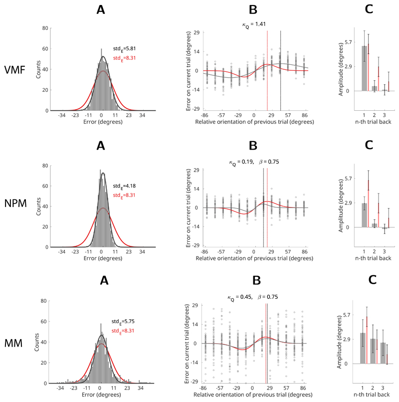
The best fitting VMF could not successfully replicate any of the three statistical effects. The distribution of errors was centred around zero but its concentration was significantly different from human data (Fig 8A-VMF, p = 0.026). Similarly, the maximum of the simulated recency bias was significantly removed from the human data (ca 20 deg for humans; ca 45 deg for the VMF; Fig 8B-VMF). Furthermore, it can be shown that the VMF cannot even theoretically have a maximum of the bias at less than π/4 radians (or 45 deg), which means it is incapable of replicating the DoG-like curve of the human recency bias (see Von Mises filter properties in Supporting Information). The VMF also could not replicate recency biases for stimuli presented 2 or 3 trials ago (Fig 8C-VMF). In sum, the VMF can simulate a recency bias but it is qualitatively different from human bias and only extends one trial back.

Figure 8. Results.

Comparison of model simulation results (black) with human data from Experiment 1 (red, Fischer & Whitney, 2014). (A) Error histograms: black – model simulation, red – average human participant. Solid lines depict Von Mises fits to error distributions. (B) Recency bias: black circles show errors of the simulated responses. Solid black line shows a DoG curve fit to the simulated errors, red line shows the human recency bias (average DoG fit to human errors). Dotted vertical lines show the location of the maxima of the recency biases (black – model; red – human participants). (C) Average recency bias amplitude computed for stimuli presented one, two and three trials back from the present. Grey bars – model; red bars – human participants. Error bars represent ±1 standard deviation of the bootstrapped distribution.

Natural prior model (NPM)

The NPM could only partially replicate the behavioural effects. The error distribution was centred around zero but significantly different from participants’ data (Fig 8A-NPM, p < 0.001). However, because NPM’s prior and posterior distributions are not Von Mises it was able to capture the DoG shaped curve of the recency bias (Fig 8B-NPM). The NPM was still not able to capture either the amplitude of the recency bias or extend it back more than one previous trial (Fig 8C-NPM). This was to be expected since the NPM, like the VMF, also predicts the next state based only on the previous one (first order Markovian). In sum, the NPM was able to replicate the DoG shaped recency bias curve but only for stimuli one trial back. Furthermore, the error distributions simulated by the NPM were significantly different from participants’ average with variance of the response reduced by approximately twofold.

Mixture model

The mixture model was able to successfully simulate all three statistical effects of interest: the distribution of errors was not significantly different from the participants’ data (Fig 8A-MM, p = 0.23); the recency bias fit the DoG-shaped curve (Fig 8B-MM), and a significant recency bias was evident over multiple past states (Fig 8C-MM). Importantly, the best-fitting β parameter value for the mixture model was β = 0.75, which effectively sets the time window for the mixture distribution at 3-4 past states (see Fig 7A, column 2, β = 0.7).

Discussion

In this paper we investigated the internal model of the environment which leads people to show a recency bias.

First, we showed that participants cannot be using a simple Bayesian filter that predicts the orientation on the current trial based only on the previous one. Furthermore, we showed that a first-order identity model is theoretically incapable of producing the recency bias observed in the orientation estimation task. This suggests that previous proposals that a simple first-order Bayesian model (such as Kalman or Von Mises filters) could explain the temporal continuity over trials and hence the recency bias (Burr & Cicchini, 2014; Wolpert & Ghahramani, 2000; Rao, 1999) are misplaced. Second, we showed that a more complex model, where participants use the natural statistics of the environment in addition to the previous stimulus, is similarly incapable of simulating the recency bias. Although such an approach is significantly better at replicating the DoG like shape of the recency bias curve it still lacks a mechanism to extend the bias beyond the most recent state. Finally, we showed that a model where the prediction about the next stimulus incorporates information from multiple past orientations can successfully simulate all aspects of the recency bias. Specifically, the participant’s model of the environment is assumed to be a mixture of multiple past states so that more recent states contribute more than older ones.

The classical Bayesian interpretation of our results suggests that the recency bias is a result of model mismatch: people infer an incorrect model for data resulting in suboptimal inference. This view posits that people are either incapable of recognising randomness or inevitably assume a model for the data since it is an efficient strategy for the natural environment, where random data is rare (Bar-Hillel & Wagenaar, 1991). Specifically, if a recency-weighted prediction works well in the natural environment, where temporal continuity prevails, people would also wrongly apply that model to random data. However, a more parsimonious explanation exists. Perhaps, rather than inferring the wrong model (out of many models that might be inferred), the recency bias may simply be a consequence of the way past experiences are represented in memory.

This can be made explicit in the framework of Bayesian filtering: the prediction for the next state is calculated by applying a state transition function a(·) to m past states:

$$z_t=a\left(z_{t-1},\dots ,z_{t-m}\right)+q,$$

where q is state noise. According to the model mismatch explanation the state transition function a(·) is the recency-weighed mixture function (Eq 7). Importantly, this assumes that all data from past m states is potentially available for the state transition function a(·) to generate a prediction. Participants suboptimal behaviour is hence caused by applying the mixture model to data representing past m states. However, exactly the same prediction would be generated if the state transition function a(·) would not perform any transform at all – is identity – but the data from the past m states is itself a recency weighed mixture. This is a more realistic interpretation since the former hypothesis assumes unlimited storage for past experiences. Similary, the latter interpretation does not require any model selection at all (out of possibly infinite models) and is hence a more parimonious view.

Consider what happens when the model of the environment is unknown and needs to be inferred in real time: for random data, such model inference is always bound to end in failure as no model can explain, compress, or more efficiently represent random input. The most efficient representation of a random latent variable is the data itself and not data plus model. In other words, people might not be applying the wrong model to the data, rather they may be failing to apply any model at all. The recency-weighted bias over multiple past states instead reflects the observer’s representation of the past. This is in agreement with previous proposals that stimulus representation in visual estimation tasks might include partially ’overwriting’ previous representations with newer ones (Matthey, Bays, & Dayan, 2015). Note that abandoning Bayesian inference altogether by simply ignoring the previous states would actually result in optimal performance in the task with random data. However, this strategy would immediately run into trouble should a pattern begin to emerge in data which is initially random.

Therefore we propose that instead of having the data and just applying a ’wrong’ model to it – a classic case of Bayesian model mismatch - the recency bias emerges because participants are continuously and unsuccessfully attempting to infer a model based on previous states. In formal terms, the state transition model contains no information (it is identity) and hence the predictive prior distribution simply reflects the observer’s representation of the past.

In sum, our results indicate that the recency bias that appears when participants are confronted with random data must be driven by a mixture of past states. We suggest that the most parsimonious explanation of our results is that participants fail to infer a model for the data and fall back on treating the internal representation of the data itself as the best prediction for the future.

References

- Anderson JR, Milson R. Human memory: An adaptive perspective. Psychological Review. 1989;96(4):703. [Google Scholar]
- Anderson JR, Schooler LJ. Reflections of the environment in memory. Psychological science. 1991;2(6):396–408. [Google Scholar]
- Bar-Hillel M, Wagenaar WA. The perception of randomness. Advances in Applied Mathematics. 1991;12(4):428–454. doi: 10.1016/0196-8858(91)90029-I. [DOI] [Google Scholar]
- Berchtold A, Raftery A. The Mixture Transition Distribution Model for High-Order Markov Chains and Non-Gaussian Time Series. Statistical Science. 2002;17(3):328–356. doi: 10.1214/ss/1042727943. [DOI] [Google Scholar]
- Bishop CM. Pattern recognition and machine learning. Cambridge University Press; 2006. 13 Sequential Data; pp. 605–652. [Google Scholar]
- Burr D, Cicchini GM. Vision: Efficient adaptive coding. Current Biology. 2014;24(22):R1096–R1098. doi: 10.1016/j.cub.2014.10.002. [DOI] [PMC free article] [PubMed] [Google Scholar]
- Cicchini GM, Anobile G, Burr DC. Compressive mapping of number to space reflects dynamic encoding mechanisms, not static logarithmic transform. Proceedings of the National Academy of Sciences of the United States of America. 2014;111(21):7867–72. doi: 10.1073/pnas.1402785111. [DOI] [PMC free article] [PubMed] [Google Scholar]
- Dubé C, Zhou F, Kahana MJ, Sekuler R. Similarity-based distortion of visual short-term memory is due to perceptual averaging. Vision Research. 2014;96:8–16. doi: 10.1016/j.visres.2013.12.016. [DOI] [PMC free article] [PubMed] [Google Scholar]
- Fischer J, Whitney D. Serial dependence in visual perception. Nature Neuroscience. 2014 Mar;17(5):738–743. doi: 10.1038/nn.3689. [DOI] [PMC free article] [PubMed] [Google Scholar]
- Fiser J, Berkes P, Orbán G, Lengyel M. Statistically optimal perception and learning: from behavior to neural representations. Trends in cognitive sciences. 2010 Mar;14(3):119–30. doi: 10.1016/j.tics.2010.01.003. [DOI] [PMC free article] [PubMed] [Google Scholar]
- Fritsche M, Mostert P, de Lange FP. Opposite effects of recent history on perception and decision. Current Biology. 2017;27(4):590–595. doi: 10.1016/j.cub.2017.01.006. [DOI] [PubMed] [Google Scholar]
- Ghahramani Z. Probabilistic machine learning and artificial intelligence. Nature. 2015;521(7553):452–459. doi: 10.1038/nature14541. [DOI] [PubMed] [Google Scholar]
- Girshick A, Landy M, Simoncelli E. Cardinal rules: visual orientation perception reflects knowledge of environmental statistics. Nature neuroscience. 2011 Jun;4(7):926–932. doi: 10.1038/nn.2831. [DOI] [PMC free article] [PubMed] [Google Scholar]
- Griffiths T, Chater N, Kemp C, Perfors A, Tenenbaum J. Probabilistic models of cognition: exploring representations and inductive biases. Trends in cognitive sciences. 2010 Aug;14(8):357–64. doi: 10.1016/j.tics.2010.05.004. [DOI] [PubMed] [Google Scholar]
- Hubert-Wallander B, Boynton GM. Not all summary statistics are made equal: Evidence from extracting summaries across time. Journal of vision. 2015;15(4):5. doi: 10.1167/15.4.5. [DOI] [PMC free article] [PubMed] [Google Scholar]
- Kalm K. Recency-weighted Markovian inference. arXiv. 2017 Nov; Retrieved from http://arxiv.org/abs/1711.03038. [Google Scholar]
- Kalman R, Bucy R. New Results in Linear Filtering and Prediction Theory. 1961;83(1) doi: 10.1115/1.3658902. [DOI] [Google Scholar]
- Kiyonaga A, Scimeca JM, Bliss DP, Whitney D. Serial Dependence across Perception, Attention, and Memory. Trends in Cognitive Sciences. 2017;21(7):493–497. doi: 10.1016/j.tics.2017.04.011. [DOI] [PMC free article] [PubMed] [Google Scholar]
- Kurz G, Gilitschenski I, Hanebeck UD. Recursive Nonlinear Filtering for Angular Data Based on Circular Distributions. American Control Conference (ACC); 2013. pp. 5439–5445. Retrieved from http://ieeexplore.ieee.org/lpdocs/epic03/wrapper.htm?arnumber=6580688. [DOI] [Google Scholar]
- Kurz G, Gilitschenski I, Hanebeck UD. Recursive Bayesian filtering in circular state spaces. IEEE Aerospace and Electronic Systems Magazine. 2016;31(3):70–87. doi: 10.1109/MAES.2016.150083. [DOI] [Google Scholar]
- Kurz G, Gilitschenski I, Pfaff F, Drude L. libDirectional. 2015 Retrieved from https://github.com/libDirectional.
- Liberman A, Fischer J, Whitney D. Serial dependence in the perception of faces. Current Biology. 2014;24(21):2569–2574. doi: 10.1016/j.cub.2014.09.025. [DOI] [PMC free article] [PubMed] [Google Scholar]
- Manassi M, Liberman A, Chaney W, Whitney D. The perceived stability of scenes: serial dependence in ensemble representations. Scientific Reports. 2017;7(1) doi: 10.1038/s41598-017-02201-5. 1971. Retrieved from http://www.nature.com/articles/s41598-017-02201-5. [DOI] [PMC free article] [PubMed] [Google Scholar]
- Marković I, Petrović I. Speaker Localization and Tracking in Mobile Robot Environment Using a Microphone Array. Proceedings book of 40th International Symposium on Robotics(2); 2009. pp. 283–288. [DOI] [Google Scholar]
- Matthey L, Bays PM, Dayan P. A Probabilistic Palimpsest Model of Visual Short-term Memory. PLOS Computational Biology. 2015 Jan;11(1):e1004003. doi: 10.1371/journal.pcbi.1004003. [DOI] [PMC free article] [PubMed] [Google Scholar]
- Murray RF, Morgenstern Y. Cue combination on the circle and the sphere. Journal of vision. 2010 Jan;10(11):15. doi: 10.1167/10.11.15. [DOI] [PubMed] [Google Scholar]
- Pouget A, Beck JM, Ma WJ, Latham PE. Probabilistic brains: knowns and unknowns. Nature neuroscience. 2013 Sep;16(9):1170–8. doi: 10.1038/nn.3495. [DOI] [PMC free article] [PubMed] [Google Scholar]
- Raftery A. A Model for High-order Markov Chains. Journal of the Royal Statistical Society. Series B (Methodological) 1985;47(3):528–539. [Google Scholar]
- Rao RP. An optimal estimation approach to visual perception and learning. Vision research. 1999 Jun;39(11):1963–89. doi: 10.1016/S0042-6989(98)00279-X. [DOI] [PubMed] [Google Scholar]
- Sarkka S. Bayesian filtering and smoothing. Cambridge University Press; 2013. 04 Bayesian filtering equations and exact solutions. [Google Scholar]
- Wolpert DM, Ghahramani Z. Computational principles of movement neuroscience. Nature neuroscience. 2000 Nov;(3 Suppl):1212–7. doi: 10.1038/81497. [DOI] [PubMed] [Google Scholar]
Associated Data
This section collects any data citations, data availability statements, or supplementary materials included in this article.