Automated Image Quality Evaluation of Structural Brain MRI using an Ensemble of Deep Learning Networks

Abstract

Background:

Deep learning is a promising methodology for automatic detection of abnormalities in brain MRI.

Purpose:

To automatically evaluate the quality of multi-center structural brain MRI images using an ensemble deep learning (DL) model based on deep convolutional neural networks (DCNNs).

Study Type:

Retrospective

Population:

The study included 1064 brain images from 1112 autism patients and healthy controls from the Autism Brain Imaging Data Exchange (ABIDE) database. Another MRI data from 110 multiple sclerosis patients were included for independent testing.

Sequence:

T₁- weighted MR brain images acquired at 3T.

Assessment:

The ABIDE data were separated into training (60%), validation (20%), and testing (20%) sets. The ensemble DL model combined the results from three cascaded networks trained separately on the three MRI image planes (axial, coronal, and sagittal). Each cascaded network consists of a DCNN followed by a fully-connected network. Quality of image slices from each plane were evaluated by the DCNN and the resultant image scores were combined into a volume-wise quality rating using the fully-connected network. The DL predicted ratings were compared with manual quality evaluation by two experts.

Statistical Tests:

Receiver operating characteristic (ROC) curve, area under ROC curve (AUC), sensitivity, specificity, accuracy, positive (PPV) and negative (NPV) predictive values.

Results:

The AUC, sensitivity, specificity, accuracy, PPV and NPV for image quality evaluation of the ABIDE test set using the ensemble model were 0.90, 0.77, 0.85, 0.84, 0.42 and 0.96, respectively. On the CombiRx set the same model achieved performance of 0.71, 0.41, 0.84, 0.73, 0.48, and 0.80.

Conclusion:

This study demonstrated high accuracy of deep learning in evaluating image quality of structural brain MRI in multi-center studies.

INTRODUCTION

Magnetic resonance imaging (MRI) is the most commonly used radiologic modality for investigating a wide variety of neurological diseases such as Alzheimer’s, multiple sclerosis, bipolar disorder, cancer, and stroke. Unfortunately, MRI image quality can be compromised by a number of factors such as patient noncompliance, hardware imperfections, and operator errors(1). Therefore, evaluation of image quality is necessary for excluding poor quality images that could compromise diagnostic confidence and affect downstream analysis(2, 3). Visual inspection of MRI images is impractical for large datasets such as in multi-center studies. In this case, automated methods become crucial.

Automated quality assessment procedures compute specific image quality metrics (IQMs) and train a machine learning algorithm to rate image quality based on the extracted IQMs. The number of IQMs used can be as small as one or two, but can be as large as few hundreds (1, 4–9). Similar approaches have been proposed for diffusion MRI (10), functional MRI (11) and multimodal integration (12). The accuracy of these methods depends on the performance of the hand-crafted IQMs. However, crafting and selecting a suitable set of IQMs are highly subjective, and the extent to which the selected IQMs capture the majority of artifacts in multi-center datasets is yet to be proven (5). A plausible approach would be to allow the data to define their own IQMs.

Recent advances in deep learning (DL) are enhancing medical imaging. In particular, DL approaches based on deep convolutional neural networks (DCNNs) have rapidly become popular in many medical image analysis problems. The major advantage of DCNNs is their ability to self-learn the image features that in traditional algorithms are hand-engineered (13). Recent studies have demonstrated the feasibility of DCNNs for automated assessment of image quality of MR images acquired from a single site (14–16). It is unclear whether the results can be successfully generalized to multi-center datasets.

In this work, we aim to develop a robust DL model for automated image quality evaluation of 3D T1-weighted (structural) brain MRI using data from a large multicenter database. We further seek to validate the performance of the developed model in another independent image set.

MATERIALS AND METHODS

MRI Data Sets and Expert Evaluation

All the data were anonymized and waived from any IRB approval. The publicly available ABIDE dataset contains 1064 structural brain image volumes acquired on 1112 subjects17. The ABIDE study included individuals with and without autism spectrum disorder, aged between 7 to 64 years. Data were acquired at 17 different sites on different MRI scanners (Philips or GE or Siemens) with varying pulse sequence parameters and voxel dimensions (17). This heterogeneity makes the ABIDE dataset suitable for training machine learning models that generalize well to images from other sites.

The ABIDE phenotypic information includes visual quality assessment of the data by three raters. Rater 1 examined the general quality of the functional data and derivatives. Raters 2 and 3 evaluated the quality of anatomical and functional data (18). For the purpose of this study, we considered only the quality assessment of anatomical data by raters 2 and 3. We labeled the images based on the following conservative criterion: an image was labeled ‘1’ if at least one of the raters rated the image as unacceptable, otherwise it was labeled ‘0’. Based on this criterion, out of 1064 volumes with accessible data and labels in ABIDE, 132 volumes were labeled ‘1’ and 932 were labeled ‘0’.

While the ABIDE dataset was used to train, validate, and test the performance of the DL model, CombiRx database(19), was used as an independent test set to evaluate the generalizability of the DL model. CombiRx, is a multicenter phase III clinical trial with 1008 enrolled patients at baseline. The data were acquired on 1.5T and 3T Philips, GE, and Siemens scanners. Structural MRI was acquired with spatial resolution of 0.94 mm × 0.94 mm × 1.5 mm with spoiled gradient recalled echo or magnetization prepared rapid gradient echo sequences (20). A board certified neuroradiologist (AK) with 9 years of experience evaluated 110 cases randomly selected from CombiRx dataset using a custom graphical user interface developed in MATLAB (version 2017a; MathWorks). Out of 110 image volumes, 29 were labelled ‘1’ and 81 were labelled ‘0’ by the expert.

Preprocessing

Both ABIDE and CombiRx database have images with variable matrix size and resolution. To facilitate their use as input to the DL model, all images were preprocessed as follows: (i) images were re-sampled to an isotropic resolution of 1 mm³ and matrix size of 256 × 256 × 256; (ii) image intensity was normalized in the range [0, 1] to accelerate convergence during training; (iii) to minimize computational complexity, 32 slices with 5 mm gap from the middle of the volume were extracted from each volume along the three principal planes (axial, coronal, and sagittal). All preprocessing steps were coded in Matlab using the Statistical Parametric Mapping (SPM12) toolbox (http://www.fil.ion.ucl.ac.uk/spm).

Network Architecture

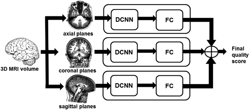
The overall process for image quality evaluation using the DL model is shown in Fig. 1. To explore the performance of the model with different image orientations, we separately trained three cascaded DL networks with inputs from axial, coronal, and sagittal slices. The extracted 32 slices along each plane were used as input to DCNN to predict the quality of each slice. The quality scores from all slices were next used as input to a fully-connected (FC) network to predict a volume-wise score. An ensemble model was constructed by averaging the quality scores from the three cascaded DL networks.

Figure 1.

Architecture of the deep learning image quality evaluation model. The extracted 32 slices along the 3 plane (axial, coronal, and sagittal) were used as input to DCNN to predict the quality of each slice. The slice quality scores were next used as input to a fully-connected (FC) network to predict the volume-wise quality. An ensemble model was constructed by averaging the image quality scores from the three cascaded networks.

The architecture of the DCNN used for assessing individual slices is shown in Fig. 2. The architecture was inspired by VGG16 model used for image classification (21), and was iteratively modified for our application and data size. The network consisted of an input layer, six convolution layers, one fully connected layer, and an output layer. The convolutional layers used 3 × 3 kernels. A 2 × 2 max pooling operation was used with a 2 × 2 stride for downsampling. The choice of the kernel size and the stride was the same as in the VGG model. The pooled feature map from the last convolutional layer was flattened into a single vector and fed to a fully-connected layer with 8 nodes. The output layer provided the slice-wise quality score. The second network for combining the slice scores into the volume score consisted of a fully-connected layer and an output layer. The networks in both stages used rectified linear unit (ReLu) as the activation function and sigmoid classification function in the last layer.

Figure 2.

Architecture of the deep convolutional neural network (DCNN) for predicting image quality of individual brain slices. conv – convolutional layer, pool – maxpooling layer, FC – fully connected layer.

Training

The ABIDE dataset was split into 638 volumes (60%, 102,144 slices) for training, 213 volumes (20%, 20,448 slices) for validation, and 213 (20%, 20,448 slices) for testing. The sampling was stratified to keep the proportion of unacceptable/acceptable images as in the whole dataset (~1:7), yielding 2,528 unacceptable and 17,888 acceptable slices for training, 864 unacceptable and 5,952 acceptable slices for validation, and 832 unacceptable and 5,984 acceptable slices for testing. Data augmentation was applied to the training set to prevent overfitting (22). All image slices were augmented using zooming (range = 0.2), rotations (range = 10°), and horizontal and vertical shifting (range = 0.1) and flipping.

The network coefficients (weights and biases) were trained by optimizing the binary cross-entropy loss function with a learning rate of 0.001 and a batch size of 64 using the Adam optimizer (23) with parameters β1 = 0.9 and β2 = 0.999. The learning rate and the batch size were optimized using a grid search. To account for the imbalance in the training set, class weights of 0.57/4.03 for the acceptable/unacceptable images were used. These weights were inversely proportional to the number of images in each category. The maximum number of epochs was 500.

The models were built in Python using the Keras Library (24) and TensorFlow (25) was used as the computing backend. Training was performed using 4 NVIDIA Tesla GTX graphics processing units (GPUs) on the Maverick2 cluster at the Texas Advanced Computing Center (TACC) at Austin, Texas.

Model Evaluation

The performance of the trained models on the held-out ABDIE test set and the CombiRx data were evaluated using the receiver operating characteristic (ROC) curve. The area under the ROC curve (AUC) was computed, and sensitivity, specificity, accuracy, positive- (PPV) and negative- (NPV) predictive values were calculated at a threshold of 0.5.

RESULTS

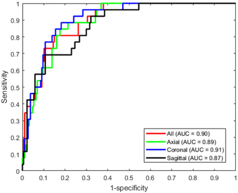
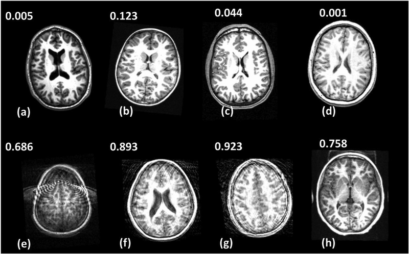
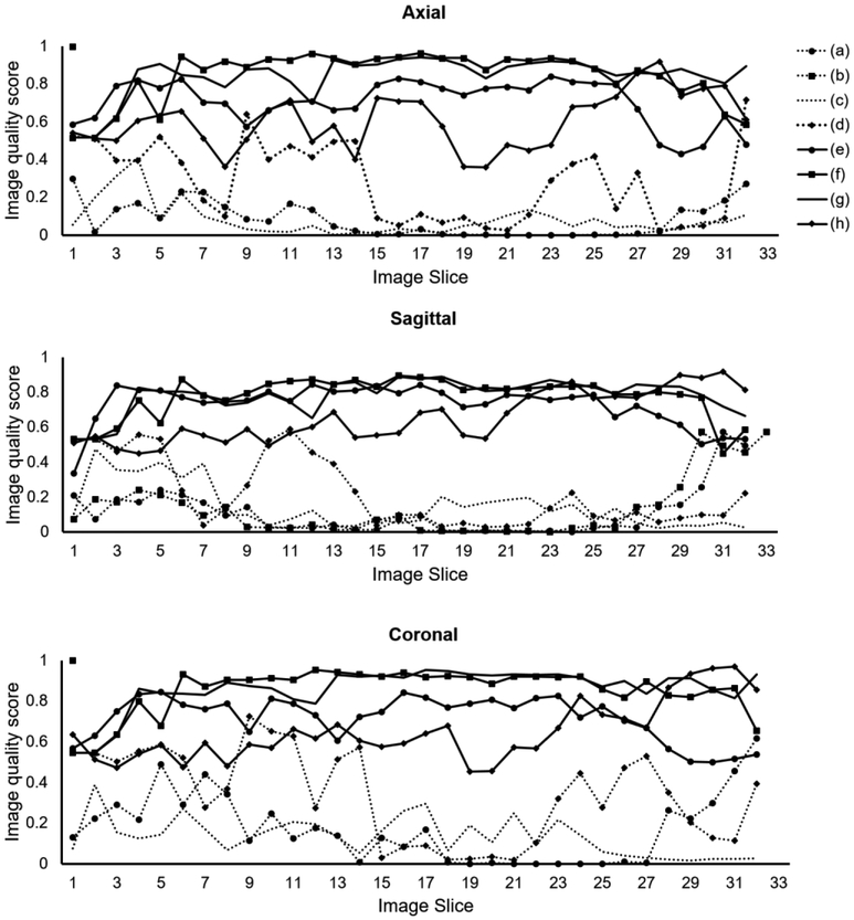
The DL model provided good accuracy for classifying brain MRI image quality as shown in the ROC curve in Fig. 3. The AUC was 0.90 for the ensemble model combining all image planes, and training using individual planes yielded AUC of 0.89 (axial), 0.91 (coronal), and 0.87 (sagittal). Fig. 4 shows images from eight different subjects from ABIDE dataset in which the DL model produced predictions in agreement with the raters, along with the predicted quality score. The individual slice scores for these images along the three planes are shown in Fig. 5, showing clustering of the quality scores of individual slices around 0 (acceptable image quality) and 1 (unacceptable quality).

Figure 3.

Receiver operating characteristic curves of the DL networks trained with individual planes and the ensemble model that averages the predictions from all planes.

Figure 4.

Concordant quality classification cases from ABIDE dataset showing images with acceptable quality (a-d) and images with unacceptable quality (e-h). The image quality scores predicted by the DL model are shown. Scores close to 0 indicate high image quality, and scores close to 1 indicate poor quality.

Figure 5.

Image quality score for individual slices of the eight sample images shown in Fig. 4 along the three image planes (axial, coronal, sagittal). (a–d) Correctly-predicted cases with acceptable image quality. (e–h) Correctly-predicted cases with unacceptable image quality.

The detailed diagnostic performance of the different quality prediction models is summarized in Table 1. In ABIDE test set, good agreement between expert evaluation and the DL model is evident with high accuracy, especially with the coronal orientation giving the highest accuracy (0.85). The highest sensitivity was obtained when the model was trained using coronal or axial images (0.81), while specificity was highest using coronal images (0.86). The ensemble model achieved similar specificity (0.85) and accuracy (0.84) as the best models, but the sensitivity (0.77) was slightly lower. When applied for predicting the image quality of the CombiRx data, the results showed comparable specificity (0.75–0.88), but lower sensitivity (0.34–0.55) and accuracy (0.67–0.75) compared to the ABIDE test set (Table 1). The sagittal orientation model provided overall better quality prediction in the CombiRx data (Table 1).

Table 1.

Performance of the developed deep learning models for image quality evaluation tested on the ABIDE and CombiRx datasets.

Database	Image planes used for training	Sensitivity	Specificity	Accuracy	PPV	NPV	AUC
ABIDE	Axial	0.81	0.82	0.82	0.39	0.97	0.89
	Coronal	0.81	0.86	0.85	0.44	0.97	0.91
	Sagittal	0.73	0.76	0.76	0.30	0.95	0.87
	All	0.77	0.85	0.84	0.42	0.96	0.90
CombiRx	Axial	0.34	0.88	0.74	0.50	0.79	0.72
	Coronal	0.45	0.75	0.67	0.39	0.79	0.69
	Sagittal	0.55	0.81	0.75	0.52	0.84	0.71
	All	0.41	0.84	0.73	0.48	0.80	0.71

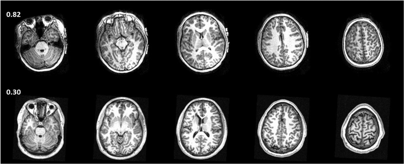
Fig. 6 shows two examples from the ABIDE test set where the prediction from the ensemble DL model did not agree with the raters. In one case, moderate motion artifacts visible on the image were missed or disregarded by both raters, but were considered severe by the ensemble DL model. The other case was labelled unacceptable, but was accepted by the DL model. Reviewing the assessment of the raters showed disagreement between the two raters in this case. In total, there were 34 cases where the prediction of DL model did not match the expert label, and among these cases raters 1 and 2 had disagreement in 12 cases (35%, Table 2). On the other hand, in the 179 cases wherein the DL model agreed with the label, the raters disagreed in 45 cases (25%).

Figure 6.

Discordant cases from ABIDE dataset. Experts labeled the image in the upper row (columns show different slices from the same subject) as acceptable quality but the DL model classified it as unacceptable (score = 0.82). There are motion artifacts evident in the images which were missed or disregarded by the experts. Images in the lower row were labelled as unacceptable by the experts, but were predicted as acceptable (score = 0.30) by DL model.

Table 2.

Agreement between raters and the DL model prediction in the evaluation of the ABIDE test set.

	Correct prediction	Incorrect prediction	Total
Raters agree	134	22	156
Raters disagree	45	12	57
Total	179	34	213

While the average training time for the DCNN was 6 hours for each plane (638 volumes), prediction of image quality for one pre-processed brain volume took less than 10 ms with the trained model.

DISCUSSION

The proposed ensemble of cascaded networks achieved high classification performance (accuracy of 0.84) on a multi-center image database acquired from different scanners and with different scan parameters. This was further confirmed by the results on an independent multicenter data acquired from another cohort. The performance on the test data from the ABIDE dataset (accuracy of 0.84) was better than the independent test set from the CombiRx data (accuracy of 0.73). This can be attributed to the differences in patient cohorts in the two studies (autism/control vs. multiple sclerosis). Training a model using both datasets may outperform the reported model because of the increased sample size and feature representation. However, we are more concerned about testing the model on an entirely different dataset to demonstrate the generalizability of our model. The CombiRx data which was acquired with different 3D protocol on an entirely different patient cohort is ideal for testing our model, and the good accuracy demonstrates reasonable level of generalizability of our model.

The performance of our DL model on multi-center image databases is comparable to traditional machine learning methods (Table 3), but the DL model avoids the need to hand-craft quality features. However, care must be taken when comparing the results from different studies. Studies almost always differ in the type of images, datasets used for training and evaluation, and how performance is measured and reported.

Table 3.

Performance of automated classical machine learning (ML) and deep leaning (DL) methods for image quality assessment.

Reference	Image type	Multi-center data?	Learning algorithm (number of features)	Sensitivity	Specificity	Accuracy	PPV	NPV	AUC
(4)	T1w, Brain	Yes	ML (2)	0.87	0.85	-	-	-	0.93
(7)	T1w, Brain	No	ML (6)	0.70	0.88	0.80	-	-	-
(27)	T1w, Brain	Yes	ML (64)	0.28	0.95	0.76	-	-	0.70
(5)	T1w, Brain	Yes	ML (190)	0.91	0.84	0.84	0.09	0.99	-
(14)	T1w, head	No	DL	-	-	0.92±0.08	-	-	-
(14)	T1w, upper abdomen	No	DL	-	-	0.72±0.05	-	-	-
(15)	T2w, Liver	No	DL	0.47 – 0.67	0.80 – 0.81	0.73 – 0.79	0.36	0.86 – 0.94	-
(16)	T1w, Brain	No	DL	-	-	0.88	-	-	-
This work	T1w, Brain	Yes	DL	0.77	0.85	0.84	0.42	0.96	0.90

Empty cells indicate values were not reported.

Mortamet et al achieved high sensitivity (0.87) and specificity (0.85) on a multi-center study using two image quality metrics based on background signal and simple thresholding(4). However, only 7.2% of the cases were of unacceptable image quality. Alfaro-Almagro et al.,(5) reported high sensitivity (0.91) and specificity (0.84) in the multi-center UK BioBank study using the QAP pipeline(26) . They developed a set of 190 IQMs to train three different classifiers: Bayes Network, Naïve Bayes and MetaCost. They achieved high sensitivity (0.91) and specificity (0.84) but with a relatively low PPV of 0.09. The classification accuracy of the MRIQC pipeline (64 IQMs and random forest classifier) described by Esteben et al., achieved satisfactory accuracy (0.76) on a single center held-out dataset(27). However, the sensitivity (0.28) was rather low. Pizarro et al.,(7) achieved good accuracy (0.80) in evaluating the image quality in a single center study using three volumetric and three artifact-specific features and a support vector machine classifier. All these methods have assessed image quality using hand-crafted image quality metrics, whose selection is subjective, and their computation can be very time consuming. In contrast, DL uses multi-resolution image features learnt from the image data.

The high performance achieved using our model supports the emerging role of DL in image quality assessment as reported in recent studies for automated detection of motion artifacts in head and abdomen MRI (14), automated image quality evaluation of T2-weighted liver MRI (15), and detection of motion artifacts in brain MRI (16) (Table 3).

Training of the DL model was very time consuming (6 hours). However, the rapid prediction time, once the network is trained, would be of help to MRI technologists in rapid screening for real-time image quality evaluation. Depending on the application, the decision threshold can be optimized to provide more sensitive or specific quality scores.

Although 3D networks could directly produce a quality score and eliminate the need for combining scores from individual slices, we elected to use 2D networks because they allow evaluating different image orientation. In addition, they have higher computational efficiency, requiring much less memory and processing power for training compared to 3D networks. While using image patches can reduce the memory requirements for 3D networks, combining the individual patch scores will still be needed. In addition, selecting the best patch size may not be trivial. Similar to a previous model (16), our model evaluates the quality along the three axes. However, our model uses full 2D slices, and not image patches, allowing the network to learn a global representation of the image.

In this work we used a binary classification of image quality into acceptable or unacceptable classes. However, a three-class classifier offers a class for ambiguous cases with discordant rater scores. In practice, we notice that both the ambiguous and unacceptable classes trigger the same course of actions: manual inspection of the images. We therefore decided to train a binary classifier. Dealing with inconsistent labels may also be addressed using active learning (8) or perceptual difference model (28).

Many of the automated quality assessment has focused on structural (3D) MRI. However, because 2D scans still present most of the clinical MRI, it is important to investigate application of implemented DL solutions to the evaluation of the quality of 2D images. The challenges of applying the implemented network for 2D images include the anisotropic resolution in 2D scans, which may results in substantially different image features other than the ones learned from thinner slices in 3D scans. In addition, application to other image contrast (e.g. T2-weighted or FLAIR, images) requires re-training to learn these contrast-specific features.

This study has its limitations. The developed DL model determines whether the image is of acceptable quality, but it does not provide information on the type of the artifact (motion, low contrast, wrap-around, etc.), nor does it provide any spatial localization of the artifact. Other models need to be developed to address these challenges. Improvements in DL performance can be achieved by using larger training datasets and better reference standards consisting of interpretations provided by multiple experts, and better ways for combining predictions from multiple planes. Further studies are necessary to transfer these results to other MR images such as T2-weighted, FLAIR, diffusion-weighted images etc. and other regions of the body.

In conclusion, we have demonstrated the feasibility of fully automated DL image quality evaluation for structural brain MRI. While these initial results are promising, further validation is necessary before it can be fully integrated into clinical practice.

REFERENCES

- 1.Osadebey M, Pedersen M, Arnold D, Wendel-Mitoraj K: Image Quality Evaluation in Clinical Research: A Case Study on Brain and Cardiac MRI Images in Multi-Center Clinical Trials. IEEE J Transl Eng Heal Med 2018; 6:1–15. [DOI] [PMC free article] [PubMed] [Google Scholar]
- 2.Reuter M, Tisdall MD, Qureshi A, Buckner RL, van der Kouwe AJW, Fischl B: Head motion during MRI acquisition reduces gray matter volume and thickness estimates. Neuroimage 2015; 107:107–115. [DOI] [PMC free article] [PubMed] [Google Scholar]
- 3.Alexander-Bloch A, Clasen L, Stockman M, et al. : Subtle in-scanner motion biases automated measurement of brain anatomy from in vivo MRI. Hum Brain Mapp 2016; 37:2385–2397. [DOI] [PMC free article] [PubMed] [Google Scholar]
- 4.Mortamet B, Bernstein MA, Jack CR, et al. : Automatic quality assessment in structural brain magnetic resonance imaging. Magn Reson Med 2009; 62:365–372. [DOI] [PMC free article] [PubMed] [Google Scholar]
- 5.Alfaro-Almagro F, Jenkinson M, Bangerter NK, et al. : Image processing and Quality Control for the first 10,000 brain imaging datasets from UK Biobank. Neuroimage 2018; 166:400–424. [DOI] [PMC free article] [PubMed] [Google Scholar]
- 6.Cameron C, Yassine B, Carlton C, et al. : The Neuro Bureau Preprocessing Initiative: open sharing of preprocessed neuroimaging data and derivatives. Front Neuroinform 2013; 7. [Google Scholar]
- 7.Pizarro RA, Cheng X, Barnett A, et al. : Automated Quality Assessment of Structural Magnetic Resonance Brain Images Based on a Supervised Machine Learning Algorithm. Front Neuroinform 2016; 10. [DOI] [PMC free article] [PubMed] [Google Scholar]
- 8.Küstner T, Gatidis S, Liebgott A, et al. : A machine-learning framework for automatic reference-free quality assessment in MRI. Magn Reson Imaging 2018; 53:134–147. [DOI] [PubMed] [Google Scholar]
- 9.Woodard JP, Carley-Spencer MP: No-Reference Image Quality Metrics for Structural MRI. 2006. [DOI] [PubMed] [Google Scholar]
- 10.Hasan KM: A framework for quality control and parameter optimization in diffusion tensor imaging: theoretical analysis and validation. Magn Reson Imaging 2007; 25:1196–202. [DOI] [PMC free article] [PubMed] [Google Scholar]
- 11.Greve DN, Mueller BA, Liu T, et al. : A novel method for quantifying scanner instability in fMRI. Magn Reson Med 2011; 65:1053–1061. [DOI] [PMC free article] [PubMed] [Google Scholar]
- 12.Abe S, Irimia A, Van Horn JD: Quality control considerations for the effective integration of neuroimaging data In Lect Notes Comput Sci (including Subser Lect Notes Artif Intell Lect Notes Bioinformatics). Volume 9162 Springer, Cham; 2015:195–201. [Google Scholar]
- 13.Litjens G, Kooi T, Bejnordi BE, et al. : A survey on deep learning in medical image analysis. Med Image Anal 2017; 42:60–88. [DOI] [PubMed] [Google Scholar]
- 14.Küstner T, Liebgott A, Mauch L, et al. : Automated reference-free detection of motion artifacts in magnetic resonance images. Magn Reson Mater Physics, Biol Med 2018; 31:243–256. [DOI] [PubMed] [Google Scholar]
- 15.Esses SJ, Lu X, Zhao T, et al. : Automated image quality evaluation of T 2-weighted liver MRI utilizing deep learning architecture. J Magn Reson Imaging 2018; 47:723–728. [DOI] [PubMed] [Google Scholar]
- 16.Fantini I, Rittner L, Yasuda C, Lotufo R: Automatic detection of motion artifacts on MRI using Deep CNN In 2018 Int Work Pattern Recognit Neuroimaging. IEEE; 2018:1–4. [Google Scholar]
- 17.Di Martino A, Yan C-G, Li Q, et al. : The autism brain imaging data exchange: towards a large-scale evaluation of the intrinsic brain architecture in autism. Mol Psychiatry 2014; 19:659–67. [DOI] [PMC free article] [PubMed] [Google Scholar]
- 18.Zarrar S, Steven G, Qingyang L, et al. : The Preprocessed Connectomes Project Quality Assessment Protocol - a resource for measuring the quality of MRI data. Front Neurosci 2015; 9. [Google Scholar]
- 19.Lublin FD, Cofield SS, Cutter GR, et al. : Randomized study combining interferon and glatiramer acetate in multiple sclerosis. Ann Neurol 2013; 73:327–340. [DOI] [PMC free article] [PubMed] [Google Scholar]
- 20.Narayana PA, Govindarajan KA, Goel P, et al. : Regional cortical thickness in relapsing remitting multiple sclerosis: A multi-center study. NeuroImage Clin 2013; 2:120–131. [DOI] [PMC free article] [PubMed] [Google Scholar]
- 21.Simonyan K, Zisserman A: Very Deep Convolutional Networks for Large-Scale Image Recognition. 2014. [Google Scholar]
- 22.Krizhevsky A, Sutskever I, Hinton GE: ImageNet Classification with Deep Convolutional Neural Networks. 2012:1097–1105. [Google Scholar]
- 23.Kingma DP, Ba J: Adam: A method for stochastic optimization. arXiv Prepr arXiv14126980 2014. [Google Scholar]
- 24.Chollet F, et al. : Keras: The python deep learning library. Astrophys Source Code Libr 2018. [Google Scholar]
- 25.Abadi M, Barham P, Chen J, et al. : Tensorflow: a system for large-scale machine learning. In OSDI. Volume 16; 2016:265–283. [Google Scholar]
- 26.Zarrar S, Steven G, Qingyang L, et al. : The Preprocessed Connectomes Project Quality Assessment Protocol - a resource for measuring the quality of MRI data. Front Neurosci 2015; 9. [Google Scholar]
- 27.Esteban O, Birman D, Schaer M, Koyejo OO, Poldrack RA, Gorgolewski KJ: MRIQC: Advancing the automatic prediction of image quality in MRI from unseen sites. PLoS One 2017; 12:e0184661. [DOI] [PMC free article] [PubMed] [Google Scholar]
- 28.Miao J, Huo D, Wilson DL: Quantitative image quality evaluation of MR images using perceptual difference models. 2008. [DOI] [PMC free article] [PubMed] [Google Scholar]