The role of aseismic slip in hydraulic fracturing–induced seismicity

Hydraulic fracturing accelerates fault creep in stable formations, loading unstable fault regions, resulting in dynamic rupture.

Abstract

Models for hydraulic fracturing–induced earthquakes in shales typically ascribe fault activation to elevated pore pressure or increased shear stress; however, these mechanisms are incompatible with experiments and rate-state frictional models, which predict stable sliding (aseismic slip) on faults that penetrate rocks with high clay or total organic carbon. Recent studies further indicate that the earthquakes tend to nucleate over relatively short injection time scales and sufficiently far from the injection zone that triggering by either poroelastic stress changes or pore pressure diffusion is unlikely. Here, we invoke an alternative model based on recent laboratory and in situ experiments, wherein distal, unstable regions of a fault are progressively loaded by aseismic slip on proximal, stable regions stimulated by hydraulic fracturing. This model predicts that dynamic rupture initiates when the creep front impinges on a fault region where rock composition favors dynamic and slip rate weakening behavior.

INTRODUCTION

Hydraulic fracturing is a process of injecting pressurized fluids into a rock formation to create open fracture systems and is used extensively in the development of low-permeability hydrocarbon reservoirs (1). Such fine-grained reservoir rocks (often referred to as “shales” for simplicity because of their fine-grained nature) are typically characterized by exceedingly low matrix permeability, typically on the order of 10⁻¹⁸ to 10⁻²¹ m² (2, 3), in addition to elevated clay and total organic carbon (TOC). Hydraulic fracture growth is generally accompanied by low moment magnitude (M_w < 0) microseismic events (1), and the occurrence of potentially damaging earthquakes was, until recently, considered unlikely (4). Hydraulic fracturing–induced earthquakes up to M_w 4.8 have now, however, been documented in China, North America, and the United Kingdom (Fig. 1A) (5–8).

Fig. 1. Global occurrences of hydraulic fracturing–induced seismicity and potential models.

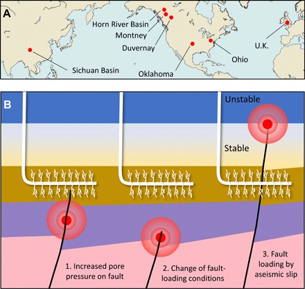
(A) Map of global reported seismicity induced by hydraulic fracturing with M_w > 3.0 (i.e., events that can likely be felt at surface). Study area is located in the Duvernay region. (B) Three models proposed for fault activation due to hydraulic fracturing, including our new model (3) [adapted from (27)].

Several models have been proposed to explain the mechanisms of fault activation by fluid injection. The first hypothesis is an increase in pore pressure within the fault zone, which leads to a reduction in effective normal stress acting on the fault (Fig. 1B) (7, 9, 10). Increased pore pressure by hydraulic fracturing is expected because (by design) the fluid pressure within a hydraulic fracture must exceed the in situ minimum stress; however, pressure diffusion away from an induced fracture is strongly inhibited by the low permeability of shales (2, 3). This fault activation mechanism therefore requires the existence of a hydrologic connection between a hydraulic fracture system and a fault, either by direct intersection (11) or, more tortuously, via naturally occurring fractures. An alternative hypothesis posits that fault activation is caused by stress changes arising from poroelastic coupling between hydraulic fractures and the rock matrix (12). This mechanism is capable of altering fault-loading conditions without any hydraulic connection (Fig. 1B), but the magnitude of the stress change is relatively small and diminishes with distance (13).

Several lines of evidence indicate that earthquake nucleation due to hydraulic fracturing is vertically offset from the injection zone. High-resolution monitoring observations indicate that hypocenters of hydraulic fracturing–induced earthquakes do not coincide with the injection depth (14–17). Moreover, laboratory measurements and in situ experiments indicate that slip on a shale-hosted fault is expected to be stable (18–20). This stability arises, in part, from the rate-state frictional parameters of rocks with high TOC and clay (19). Together, these observations imply that if the first hypothesis is correct, then dynamic rupture arises from along-fault diffusion of pore pressure, whereas the second hypothesis favors rupture nucleation relatively close to the injection zone.

Here, we consider a third hypothesis that distal dynamic rupture is induced by pore pressure–driven aseismic slip, which propagates from the reservoir depth out to the seismogenic region of the fault (Fig. 1B). The idea of an aseismic slip front outpacing a pore pressure diffusion front has been previously proposed (10, 21, 22), with recent laboratory (centimetric scale) and in situ observations at the decametric scale confirming that aseismic slip in pressurized regions of faults can activate slip along nonpressurized fault patches (23–26). Here, we apply the same model but at a much larger scale, i.e., to a kilometer-scale fault rupture that has been linked to hydraulic fracturing (27, 28).

To test this hypothesis, we analyze an unusually comprehensive dataset from central Alberta, Canada (“Duvernay,” Fig. 1A). Since December 2013, several notable earthquakes in this region have been linked in space and time with hydraulic fracturing programs (29). The focus of our study is a M_w 4.1 event on 12 January 2016, currently one of the largest magnitude seismic events induced by hydraulic fracturing (7, 17, 27, 28). Hydraulic fracturing in this region is focused on the Late Devonian Duvernay Formation (Fig. 2), which is composed of multicyclic units of organic-rich shales and fine-grained carbonates (30). Precambrian basement is inferred to be located ~400 m below the reservoir (27), while immediately above the Duvernay is the Ireton Formation, which is primarily composed of clays alternated with fine-grained carbonates (31). These units are conformably overlain by carbonate-rich rocks of the Winterburn and Wabamun groups (Fig. 2A).

Fig. 2. Data used to derive rate-state model parameters.

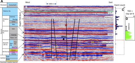
(A) Stratigraphic column from the study area (blue, limestone and dolostone; gray, shale and mudstone; orange, sandstone; pink, evaporites). (B) West-east slice through a 3D seismic volume (vertical exaggeration, 4.25; see Fig. 3 for location), showing the location of the M_w 4.1 earthquake (red star). TVD, total vertical depth from surface. Several north-south–oriented faults can be distinguished (black lines), including one coincident with the location of the earthquake. C, possible channel visible as a “bowtie” structure; SR, edge of Swan Hills Formation reef structure. (C) Histogram of seismic event locations versus depth for 20-m bins (red asterisk, M_w 4.1 earthquake; red dashed line, treatment well depth). (D) Estimated TOC + clay weight percentage derived from well log data.

RESULTS

Figure 2 shows a profile extracted from the three-dimensional (3D) seismic volume through the location of the M_w 4.1 earthquake (see Fig. 3A for profile location). Several subvertical faults are identified (see Materials and Methods). One inferred basement-rooted fault strand coincides with the location of the mainshock, cutting through both the injection zone and the seismogenic region. A graph of TOC + clay weight percentages (Fig. 2C), derived from nearby well log data (fig. S3), shows a sharp transition from high values (>30%, corresponding to stable sliding regime) in the Duvernay and Ireton to approximately zero (corresponding to potentially unstable sliding) at shallower depths. Similarly, a depth histogram of seismicity (Fig. 2C) shows that most of the seismic activity occurs within the unstable sliding Wabamun and Winterburn carbonate units.

Fig. 3. Microseismic monitoring data from a treatment associated with a M_w 4.1 earthquake.

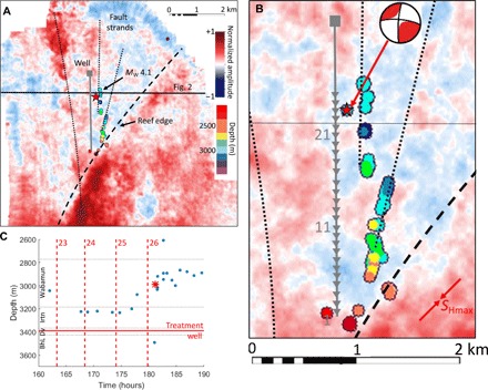
(A) Depth slice through the 3D seismic volume showing normalized seismic reflection amplitude at the level of the Beaverhill Lake Group (at 3386-m depth; Fig. 2), which directly underlies the Duvernay Formation (gray line, treatment well location; black solid line, profile in Fig. 2; red star, M_w 4.1 earthquake). Various structural features can be interpreted, including the edge of the Swan Hills reef structure and a series of roughly north-south lineaments. Seismic event locations are overlain, colored by depth. (B) Enlargement of (A) around the treatment well [triangles, injection stages (numbered at intervals)]. Focal mechanism of the M_w 4.1 event (27) is shown as a beach ball. Approximate orientation of maximum horizontal stress is labeled (S_Hmax); hydraulic fractures should grow parallel to this direction (1). (C) Depth of the seismic events versus time for the events in the immediate vicinity of the mainshock [red dashed lines, stage start times; black dotted lines, stratigraphy according to a well log ~3 km north (BhL, Beaverhill Lake; Dv, Duvernay; Irtn, Ireton); red star, M_w 4.1 earthquake].

Figure 3 shows a map of seismicity recorded during the hydraulic fracturing treatment associated with the M_w 4.1 event (see fig. S1 for more details and for cross sections); seismic events are overlain onto a 3D seismic time slice through the mid-Devonian Beaverhill Lake Group, which forms a substrate to the reservoir and contains a reef margin that marks a lithologic boundary between shale and carbonate (see Materials and Methods). The event distribution outlines several rectilinear trends that correlate with linear features in the 3D seismic image (Fig. 3, A and B). These trends are very similar to those observed using a dense microseismic monitoring array (17). We interpret these linear features as anastomosing strands within a regional strike-slip fault system (17, 27, 28). Apparent truncation of the linear features by the reef edge implies that only limited (<50 m) net slip has accumulated on these faults since reef growth in the mid-Devonian. The seismic event distribution is uncharacteristically asymmetric and is concentrated on the east side of the well, suggesting the presence of a lateral stress gradient due to the influence of nearby faults (32). Figures 3C and 4 show updip progression of seismicity leading up to the M_w 4.1 earthquake, culminating in a mainshock and aftershock sequence at a depth of ~3000 m (Fig. 4 shows propagation upward along the fault plane). The mainshock occurred on a north-south–oriented fault, which is parallel to the treatment well (17). They are both oriented ~45° from the maximum horizontal stress (Fig. 3) (27); thus, there is substantial resolved shear stress on the fault [treatment wells are often drilled perpendicular to the maximum horizontal stress (1); however, in this case, the well orientation was determined by the shape of the land lease boundary].

Fig. 4. Foreshocks and aftershocks of the M_w 4.1 earthquake over time in west-east cross section.

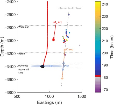
Timing of the M_w 4.1 earthquake is highlighted in red. Treatment well (red line), stage locations (black triangles), stratigraphy (black dotted lines), and estimated positions of the steeply dipping fault plane and region of increased pore pressure due to hydraulic fracturing (HF) are shown. Creep outpaces the pore pressure diffusion (PPD) front on the fault plane. The mainshock is believed to be located on the same fault plane as the other events but is slightly mislocated horizontally because of the lower frequency content.

The spatial and temporal evolution of seismicity leading up to the mainshock, coupled with the interpreted fault geometry and log signatures, are consistent with upward propagation of an aseismic deformation front, followed by initiation of dynamic rupture where the deformation front impinges on unstable regions of the fault (Fig. 4). To simulate slip activation and development on the near-vertical north-south fault observed in the 3D seismic and microseismic data, we performed 1D rate-state friction modeling (Fig. 5) (33, 34) constrained using input parameters from a range of available data (fig. S3 and Materials and Methods) and the hydraulic fracturing stage schedule (fig. S4 and table S1). The model was initialized by considering long-term fault creep due to reservoir overpressure generation on a time scale of tens of millions of years (35). Observed overpressure is mainly confined to the frictionally stable shales (figs. S3 and S5), resulting in preloading of fault stress in the adjacent strata (fig. S5). During hydraulic fracturing, the model shows that accelerated aseismic fault creep results from pressure increases where the hydraulic fractures intersect the fault. The stress transfer arising from aseismic slip substantially outpaces the pore pressure diffusion front, even considering pore pressure–induced permeability increase on the fault (Fig. 5B and Materials and Methods). The nucleation of dynamic rupture occurs once aseismic slip has propagated ~50 m into the locked carbonate units (~250 m above the fractured well), close to the location of maximum negative (a − b) [friction rate parameter (19) estimated from the TOC + clay results]. In the numerical simulation, a M_w 4.1 earthquake is generated at the beginning of stage 24, exhibiting magnitude and timing that are similar to the observed event (see Materials and Methods for a detailed description of the dynamic rupture propagation). Essential to this coseismic slip model is the propensity of carbonate fault gouge to undergo a near-complete dynamic weakening, owing to a process such as flash heating–induced thermal decomposition of calcite at sliding microasperities (see Materials and Methods) (36–38) or superplastic deformation (fig. S6) (39). Numerical simulation of slip without dynamic weakening leads to a much smaller event (Fig. 5D and fig. S7).

Fig. 5. Displacement evolution on a vertical strike-slip fault intersecting the injection zone (Duvernay).

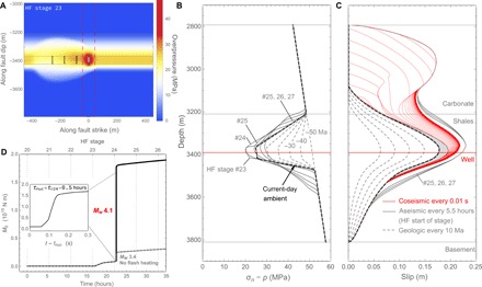
(A) Snapshot of overpressure on a vertical fault intersected by hydraulic fractures at the shut-in of stage 23 (numbered black rectangles, stages 20 to 23). Model includes pre-existing overpressure field that developed during hydrocarbon maturation. (B) Evolution of effective normal stress, averaged over the along-strike fault section centered on x = 0. Dashed contours show long-term stress evolution (adjusted to the present-day depth), while solid contours show the short-term increase due to hydraulic fracturing. Stage 27, end of stage 26. (C) Fault slip shown by gray dashed lines every 10 million years (Ma; long-term geologic creep), by continuous gray lines every 5.5 hours starting from the beginning of stage 23 (accelerated creep), and by red continuous lines every 0.01 s (coseismic slip). Total hydraulic fracturing–induced aseismic slip before the earthquake nucleation shown by the shaded area. (D) Moment release as a function of time; onset of accelerated aseismic slip at the beginning of stage 23 leads to a M_w 4.1 earthquake early into stage 24.

DISCUSSION

Improved understanding of fundamental processes of fault activation during hydraulic fracturing is key to developing effective monitoring and mitigation strategies and could also help to inform our understanding of natural earthquake triggering. Current mitigation strategies for hydraulic fracturing–induced seismicity in this region are based on the use of a traffic light protocol (40) [traffic light protocols are feedback systems that allow for an operational response to the nearby occurrence of seismic events exceeding a prescribed set of criteria (41)]. The existing system may not be optimal, as there is an implicit assumption that a large-magnitude earthquake is preceded by smaller precursory events and that changes in injection operations would have an immediate effect on the source process of induced events. According to our model, mitigation of induced seismicity may benefit more from characterizing nearby faults, state of stress (including overpressure), and rock properties (TOC, clay, and carbonate content). Furthermore, the maximum magnitude of an event may be limited by factors that include geometrical considerations (thickness of the unstable layers and vertical distance from injection zone), geological overpressure history, and slip deficit accumulated over the epoch of stable creep in the adjacent stable formations. Deployment of new technologies for direct detection of aseismic slip (such as fiber-optic distributed strain sensors) could provide a useful approach to complement traditional monitoring methods.

In a broader context, the apparent association of hydraulic fracturing–induced seismicity with faulting in carbonates is consistent with observations of some of the largest natural earthquakes occurring within the sedimentary cover worldwide (42). Similarly, interconnected, vertically stacked creep and dynamic rupture processes occur at separate depths on some faults such as the San Andreas (43), where aseismic creep has also been hypothesized as the driving process of natural earthquake swarms (44). Considering the wealth of detailed geological and operational information acquired by the hydrocarbon industry in areas of injection-induced seismicity, our findings could therefore also be beneficial to understand other induced and natural earthquake systems.

MATERIALS AND METHODS

Computing TOC + clay

The TOC (total organic carbon) + V_clay (volume of clay) weight percentages were estimated from spectral gamma ray (SGR) logs. SGR uranium content is tightly related to the TOC (45, 46), and the SGR thorium reading is a function of the amount of the clay volume present in the reservoir (46, 47). These well log–estimated empirical correlations were calibrated using the closest well with available Duvernay core for analysis, ~17 km southeast from the treatment wellhead. The cored well has available SGR logs and 29 core plugs with measured TOC (from Rock-Eval) and V_clay [from x-ray diffraction (XRD)] within the Duvernay Formation. For the correlation of SGR uranium content to TOC (in weight %), a linear function using 0.0033 as conversion factor was applied [i.e., TOC_uranium = uranium reading parts per million (ppm) × 0.33; fig. S2A]. This ensured the best correlation between the modeled TOC using well logs and the TOC directly measured on 26 core samples (R² = 0.73).

For V_clay estimation, a cross-plot of SGR thorium reading versus measured V_clay (from XRD) was built for 20 core plugs taken within the Duvernay Formation (fig. S2B). In the analyzed core, V_clay ranged from 3 to 45%, and thorium reading ranged from 3.5 to 13 ppm. The trend line fitting the 20 data points intersects 0% clay at 3 ppm (Th_min) and 100% clay at 21 ppm (Th_max). On the basis of this, we estimated V_clay weight % = (Th_reading − Th_min)/(Th_max − Th_min) with R² = 0.58.

Reflection seismic data

Migrated 3D seismic reflection data from the same acquisition program used in this study were discussed in (48). As part of the processing of the reflection seismic data, amplitude normalization was performed, such that the highest observed reflection amplitude had a value of unity. Geologic horizons shown in Figs. 2 and 3 were based on a calibration well that was drilled to a total vertical depth of 3607 m from a surface elevation of 890.9 m (48). The top of Precambrian basement is deeper than local well control and so was correlated using a nearby Lithoprobe deep reflection survey, which has synthetic ties to Precambrian well penetrations (49).

Images extracted from the 3D seismic volume can be used to investigate structural features within the region at various depths. We first flattened the reflections at the Wabamun Formation top to highlight geological features that were present before and during deposition of this layer. Figure 2B shows a cross section through the 3D seismic volume displaying seismic amplitudes as a function of depth, which can also be used to visualize structural features, as well as stratigraphy. Figure 3 (A and B) shows a horizontal slice through the 3D seismic volume at a depth of 3386 m, with the positive and negative seismic amplitudes highlighting various structural features discussed below.

Although cumulative fault displacement is inferred to be dominantly perpendicular to the horizons, subvertical faults can nevertheless be identified on the basis of localized curvature anomalies (50) or changes in apparent dip of reflections that mark the locations of hinge lines (49). Channel and reef edge features can also be identified in Fig. 2 in a similar manner; however, the interpreted fault strands span multiple stratigraphic horizons and correlate with the linear features in Fig. 3. Our estimate for maximum post–mid-Devonian fault displacement was constrained by the lack of a discernible lateral offset on the reef edge. Figure 3A shows that there is little discernible offset of the mid-Devonian Swan Hills reef margin where it is intersected by the observed faults. Some seismicity forms a cluster aligning parallel to the reef edge (17), suggesting that higher mechanical strength of the reef facies relative to the off-reef facies may have influenced faulting. The theoretical resolution limit for migrated seismic data is equal to the spatial sampling interval; thus, based on the common midpoint interval for the data of 30 m, we estimated that the offset on the reef margin can be no greater than 50 m (allowing for some uncertainty).

Broadband seismic data

The hydraulic fracturing operations associated with the M_w 4.1 event were monitored using a small network (WSK) of four industry-provided broadband stations, located between 2.4 and 7.6 km from the treatment well. The continuous ground motion recordings from these sensors are publicly available for the period between 00:00 UTC on 1 January 2016 and 1:56 UTC on 19 January 2016. A catalog containing 108 events was detected during this period, with a minimum event magnitude of M_L 0.3.

Pick times were manually extracted for P- and S-wave onsets, and a grid search was performed to minimize the difference in differential theoretical travel times between each grid point and each pair of receivers with observed differential pick times (51). Theoretical travel times were obtained using a simple ray-tracing tool and the same 1D velocity model that was used to locate the microseismic catalog (17), which was calibrated using perforation shots [explosions used to create holes in the well casing at each stage to allow egress of fracturing fluid into the surrounding medium (1)] with known locations. A 1D velocity model is a reasonable assumption given the relatively horizontal stratigraphy observed in Fig. 2. The grid search was confined to a 8.2 km by 8.5 km by 5 km volume with a 25-m resolution (in east-west, north-south, and depth, respectively), centered around the treatment well.

After obtaining the initial locations, the events were subsequently relocated using HypoDD, a double-difference relocation algorithm (52). To obtain high-precision differential pick times between events at each station, the waveforms were band-pass–filtered between 1 and 20 Hz. A 2.5-s window was taken around the catalog pick time (starting 0.05 s before the catalog pick time). For every station, differential pick times were calculated as the lag times associated with the maximum correlation coefficients for the windowed P and S phases for all events cross-correlated with the corresponding windowed phases for all other events. The pick times of each phase were adjusted accordingly, and the square of the maximum correlation coefficient for each phase was used as a weight in the HypoDD algorithm (52). The results (fig. S1) show locations that are consistent with the microseismic locations in (17), and therefore, the same structural features are apparent. The hypocenter depths are also very similar; differences in the apparent dip of the southern imaged structures are likely a manifestation of the station coverage in the broadband network. The one inconsistency is that the M_w 4.1 event is slightly offset to the west of a linear cluster of hypocenters in the northern region. Given that the microseismic data show the hypocenter of this event aligning with this cluster and that the frequency content of this event differs from that of the other events that are substantially smaller, which may adversely affect the phase correlations used in the HypoDD algorithm, we believe that this offset is caused by an error in the location of the mainshock. The true hypocenter likely aligns on the same fault strand as the observed cluster of seismicity.

Model fault geometry, ambient stress, and pore pressure

A north-south striking subvertical strike-slip fault intersecting the Duvernay Formation and other neighboring stratigraphic units is indicated by reflection seismic data and relocated microseismicity (Fig. 2 and fig. S1). The fault is assumed to terminate in the carbonate (Wabamun) formation updip at the shallowest recorded aftershocks of the M_w 4.1 event. Downdip assumed that locking depth is at the basement contact (Fig. 2) (note that this precludes simulation of possible earthquakes in the basement extension of the fault). The total fault height capable of slip is 1017 m.

The regional maximum horizontal in situ stress direction is northeast-southwest (27), at ~45° to the north-south striking fault. The minimum stress gradient of 20.78 kPa/m in the proximity of the well, and, by extension, in the proximity of the fault striking parallel to the well ~100 m to the east, is inferred from the hydraulic fracture stage 23 data (see fracture closure stress; table S1) and is within the range of 19 to 22.4 kPa/m suggested previously for the Kaybob Duvernay play (53). The same study estimates maximum stress in the Duvernay to be in the range of 27.1 to 31.7 kPa/m with the median value of 29.5 kPa/m. Corresponding fault normal and shear stresses (neglecting stress rotations near the fault) are σ_n = (σ_max + σ_min)/2 = 25.14 kPa/m and τ = (σ_max – σ_min)/2 = 4.36 kPa/m. The resulting nominal value of the fault stress ratio τ/(σ_n − p_hydrostat) = 0.29 is substantially lower than the nominal friction values of ~0.5 to 0.6 of shale and carbonate-rich fault gouges, and, if taken for the far-field fault loading, would preclude any notable fault slip outside the overpressured reservoir fault section. This deviates from a simple model of a critically stressed crust (54); however, we remark that (i) the faults appear to terminate at the top of the Late Devonian Wabamun Formation (Fig. 2) and therefore represent relic structures that formed at a time when the stress field was likely different from the present day and (ii) sedimentary basins exhibit geomechanical layering with variable stress between stronger and weaker layers, such that if the crust is critically stressed at some depths, it cannot be critically stressed throughout the sedimentary section (55). The low estimated value of the fault stress ratio in the Duvernay is consistent with the shear stress drop there because of the long-term slip along the creeping sections of the fault through overpressured shales or sandstones. Naturally occurring fault creep is the result of the long-term reservoir overpressure associated with the hydrocarbon generation coupled with the stable frictional rheology of the shale fault sections (see discussion of the fault friction and pore pressure regime below). Furthermore, this long-term slip is expected to scale the potentially seismogenic slip of the adjacent locked sections of the fault (through frictionally unstable carbonates and/or basement rocks) when triggered by anthropogenic fluid injection. For the M_w 4.1 event, rupture dimensions of ~0.4 km (dip) and ~1 km (strike) are estimated, as outlined by the spatial distribution of the early aftershocks (Fig. 3 and fig. S1), and the shear modulus of the rock of μ = 25 GPa, resulting in an estimated average seismic slip 〈δ〉 of ~ 0.15 m. Using this seismic slip as the proxy for the long-term accumulation of aseismic slip over the adjacent creeping fault section of estimated height h ~ 400 m (twice the depthwise distance from the center of the overpressured Duvernay to the contact with the seismogenic and interseismically locked carbonate), we can estimate the average long-term stress drop along the creeping section Δτ = (2/π) μ 〈δ〉/h ~ 11.9 MPa (or 3.5 kPa/m). This estimate translates to the background shear stress gradient τ_b = τ + Δτ = 7.9 kPa/m (fig. S3A) and the nominal value of the background fault stress ratio ~ 0.52.

For the ambient pore pressure distribution, we considered an overpressured Duvernay Formation sealed from the formations above and below, where a normal (hydrostatic) pore pressure distribution was modeled. This is consistent with reported drilling experiences above the Duvernay (i.e., in the Ireton) (53). The Duvernay overpressure was modeled as a pore pressure gradient of 17.7 kPa/m [within the window of 15.8 to 18.1 kPa/m (53) and the median value reported for seismogenic Duvernay plays (35)]. Expected transition zones (seals) between the overpressured Duvernay and normally pressurized formations above and below have been suggested to account for potential overpressure-related drilling problems in the Ireton (53) and potential fault-valve action and episodic release of Duvernay overpressure in the bounding formations along vertical strike-slip faults (35), such as the one studied here. We modeled these as the tapered zones between the overpressured Duvernay and normally pressured surrounding formations (fig. S2A).

Fault friction

Fault slip takes place in response to changes in the fault frictional strength τ_f = f (σ_n − p). Evolution of the friction coefficient f was modeled using the slip law formulation of the rate-state theory (56, 57) in the form of (58), which specifies friction

$$f=f_{\mathrm{o}}+a \text{ln} (V/V_{\mathrm{o}})+\mathrm{\Theta }$$ (1)

as a function of the slip rate V = dδ/dt and frictional state variable Θ. Here, f_o and V_o are reference values, and a is the direct effect coefficient. The evolution of the fault state is governed by the “distance” of the friction f from its steady-state value f_ss(V) as follows

$$d\mathrm{\Theta }/\mathit{dt}=-(V/L) (f-f_{\text{ss}}(V))$$ (2)

where L is the state evolution distance. At the steady state, a conventional logarithmic dependence on the slip rate, corroborated experimentally at low slip velocities, was used, i.e., f_ss(V) = f_LV(V) with

$$f_{\text{LV}}(V)=f_{\mathrm{o}}+(a-b)\text{ln}(V/V_{\mathrm{o}})$$ (3)

The parameters of the rate-state frictional model were constrained using laboratory friction data for reservoir shale rocks (19) and carbonates (42, 59), as well as the TOC + clay data from well logs (Fig. 2D and Materials and Methods). Duvernay shale frictional properties (also used for clastic formations downdip of Duvernay) were inferred on the basis of the friction correlation (19) to the clay + TOC gouge content. The TOC + clay content distribution interpreted from the well log analysis was highly irregular through the shales (Duvernay and Ireton), yet we observed to the first order a decreasing TOC + clay content in the updip direction toward the contact with carbonates (above which the TOC + clay was null). As a first-order model, we took the average TOC + clay content values of ~33 to 34% over the Duvernay and clay-rich downdip part of Ireton (<3318 m) and used the corresponding correlation value (19) of a − b = 0.0025 to model the steady-state friction rate dependence uniformly over the Duvernay. For the carbonate-rich gouge of the Wabamun and Winterburn formations, we used a − b = −0.0025 updip of the contact with Ireton shales, as inferred from the hydrothermal data (59) at a representative temperature of ~110°C. The final adopted depth distribution of the a − b parameter is a linear taper between the above two end-members, such that neutral velocity dependence of friction (a − b = 0) takes place at the contact between shales (Ireton) and carbonates (fig. S3B).

Reference value of friction coefficient at reference slip rate V_o = 1 μm/s was set at f_o = 0.5 in the Duvernay (19) and at f_o = 0.6 in the carbonates (59) above and in the sandstones below, while a linear taper was used in between these end-members (fig. S3B). The direct effect coefficient was modeled similarly on the basis of the adopted end-member values of a = 0.01 (shales and sandstones) (60) and a = 0.02 (carbonates) (42). For the state evolution distance, we used a uniformly distributed value of L = 100 μm (19, 59, 60).

Strong weakening of carbonate fault gouge at high slip velocity

When modeling seismic slip, we recognized the propensity of calcite-rich gouges for flash heating–induced thermal decomposition (36, 37, 61), specifically decarbonation (CO₂ release) and deposition of amorphous carbon (nano-lubrication), resulting in a dramatic drop of the steady-state friction (<0.1), with the slip velocity approaching seismic values. The rate-state frictional framework can accommodate the entire spectrum of frictional responses, from low to high slip velocity, when the steady-state friction expression is amended, e.g., as

$$f_{\text{ss}}(V)=f_{\mathrm{w}}+(f_{\text{LV}}(V)-f_{\mathrm{w}}) {(1+{(V/V_{\mathrm{w}})}^m)}^{-1/m}$$ (4)

where f_w is the flash-heated (minimum) steady-state value of the friction coefficient and V_w is a characteristic weakening velocity value, such that the steady-state friction dependence on the velocity reduces to the end-members f_LV(V) and f_w when V ≪ V_w and V ≫ V_w, respectively. Exponent m ≥ 1 in Eq. 4 is a fitting parameter, with larger values corresponding to sharper transition between the low-velocity lnV and high-velocity ~1/V dependence of the friction on V [the limit of m = ∞ corresponds to the abrupt transition between the two asymptotic behaviors (62)].

We fit the friction versus slip rate data from the laboratory slip on a marble saw cut (37) with Eq. 4 to infer f_w = 0.07, m = 6, and V_w,lab = 0.28 m/s (fig. S6, dashed line), while using the low-velocity friction f_LV(V) (Eq. 3) characterized by f_o = 0.6, V_o = 1 μm/s, a = 0.02, and a positive value for the velocity dependence coefficient (a − b)_lab = 0.0025 for calcite at room temperature (59) (as opposed to a − b = −0.0025 in situ). The flash heating theory (38) predicts that V_w scales with the square of the difference between the weakening temperature T_w for the onset of thermal decomposition and ambient temperature T. This allows the in situ value of the weakening velocity to be inferred from the laboratory value, V_w = V_w,lab (T_w − T)²/(T_w − T_lab)² = 0.2 m/s, when T_lab = 20°C, T = 110°C (in situ temperature), and T_w = 600°C [temperature at the onset of decarbonation (37)] are used. The corresponding dependence of the steady-state friction of calcite on the slip velocity under the in situ conditions is shown in fig. S6.

Fault slip modeling

To model the fault slip, we solved equations of quasi-dynamic elasticity, which relate the change of fault normal and shear tractions to slip (34).

$$\mathrm{\sigma }(z,t)–{\mathrm{\sigma }}_n(z)=0$$ (5)

$$\mathrm{\tau }(z,t)–{\mathrm{\tau }}_{\mathrm{b}}(z)=(\mathrm{\mu }/2\mathrm{\pi })\int (\mathrm{\partial }\mathrm{\delta }(z\prime ,t)/\mathrm{\partial }z\prime )dz\prime /(z-z\prime )–(\mathrm{\mu }/2c) \mathrm{\partial }\mathrm{\delta }(z,t)/\mathrm{\partial }t$$ (6)

where μ is the elastic shear modulus and c is the shear wave velocity. The shear traction on a slipping fault is given by the fault frictional strength

$$\mathrm{\tau }(z,t)=f(z,t) ({\mathrm{\sigma }}_n(z)–p(z,t))$$ (7)

and the evolution of the rate-state–dependent friction is described by Eqs. 1 to 4. We used the spectral method (63) applied to a finite fault of height H without replication (64) and fast Fourier transform to solve Eq. 6 on a grid of N nodes z_j = z_{downdip_end} + (j −1) Δz (j = 1,…,N) with uniform spacing Δz = H/N and reduce the problem to a system of dynamic ordinary differential equations (ODEs) for the values of slip at the nodes. Earthquake slip instabilities result in slip rates vastly variable in space and time, rendering the ODE system stiff (33). We overcame the numerical difficulty of solving a stiff system by changing the dynamic variable (time) to the fault-average slip. This allows the transformed ODEs to be solved using a routine solver with adaptive step in Wolfram Mathematica software.

Space discretization, convergence of the numerical solution, and creep versus pore pressure diffusion front dynamics

We used the numerical stability considerations (33, 34) for slip on the frictionally unstable (a − b < 0) part of the fault to constrain the spatial discretization Δz ≪ h* = μL/max[(b − a)(σ_n – p)] ~ 20 m on the basis of frictional properties of the carbonate units of the fault (fig. S3B).

We note that the above criterion does not place any constrain on the grid spacing from the frictionally stable (a − b > 0) part of the fault (through shales and sandstones). We therefore investigated the stability and grid dependence of the numerical method when applied to a simplified setting of aseismic slip on a frictionally stable fault (characterized by the parameters for the Duvernay section of the full fault model) subjected to a constant ambient effective normal stress of 50 MPa. In this numerical example, the fault, initially in the steady state of uniform creep at a rate of 10⁻¹⁰ m/s, undergoes an episode of accelerated aseismic creep driven by 1D pore pressure diffusion p(z,t) − p_o(z) = Δp_max Erfc(|z|/√4αt) with hydraulic diffusivity α = 0.05 m²/s from a constant overpressure Δp_max = 25 MPa source at z = 0. Figure S8 shows the development of the effective normal stress (due to the diffusive pore pressure change), shear stress change, slip rate, and slip along a finite fault of height H = 200 m (−H/2 < z < H/2) in the numerical solution with a large number of grid points N = 2⁹ (fine spatial resolution Δz = 0.39 m). The symmetric crack-like expansion of the accelerated aseismic creep is seen to substantially outpace the pore pressure diffusion, which is quantified in a more direct fashion by tracking the creep and diffusion fronts in time (fig. S8E). Here, the two fronts have been defined as the location of the peak shear stress and the location |z| = 1.3859 √4αt, where pore pressure change is 5% of Δp_max, respectively. The runout distances of the two fronts in this example are different by a factor of ~2.5 after 5 hours of fluid injection.

Carrying out the numerical solution with a reduced spatial resolution, we observed the grid independence of the results for N ≳ 2⁸ or Δz ≲ 0.8 m (fig. S8), while artificial slowdown of the creep front was evident for a coarser grid. On the basis of this example, we can conclude that, although the numerical solution for slip on the frictionally stable part of the fault remains numerically stable (obtainable) when carried out on a coarse grid, there exists a threshold spatial resolution below which the solution is grid dependent. The latter has to be considered in conjunction with the criteria in (33, 34), when solving for slip on faults with heterogeneous friction (stable and unstable parts).

The grid independence of the numerical solution for slip in our full fault model with heterogeneous friction (fig. S3B), as detailed further, has been established by direct computations of the model for N ≳ 2¹¹ (Δz ≲ 0.4 m). This spatial resolution threshold is required to fully resolve the time progression of the aseismic slip on the frictionally stable (shales) part of the fault induced by the hydraulic fracture stimulation, while the condition for grid independence of the solution for the slip on the frictionally unstable (carbonates) part of the fault is less restrictive (i.e., the slip there could, in principle, be adequately computed on a coarser grid).

Long-term creep due to the reservoir overpressure generation

Given the stable frictional rheology of shales or sandstone fault units, we anticipated that those may have undergone long-term geological creep driven by the fault stress and pore pressure loading. Specifically, we expected that the development of the current-day reservoir pore overpressure, attributed mainly to hydrocarbon generation over tens of millions of years (35), may have amplified the amount of creep in the shale section and, consequently, the stress redistribution along the fault leading to the stress concentration in the locked (frictionally unstable) fault units. We modeled the geologic creep on the fault by applying the background shear and normal stresses, as corroborated in the above, and initially hydrostatic pore pressure at t = −50 million years (Ma; with t = 0 corresponding to the present day) and by ramping up the pore overpressure linearly in time from zero to the current-day profile (fig. S5A). The resulting history of fault slip accumulation (fig. S5D) shows a maximum cumulative current-day slip of ~0.15 m coincident with maximum overpressure (Duvernay), tapering to zero updip into the “locked” carbonate (Wabamun/Winterburn) formations and downdip at the basement contact. Corresponding shear stress redistribution (fig. S5B) leads to unloading in the creeping shales and development of stress concentration in the locked carbonates. By performing additional calculations with earlier initialization time (t < −50 Ma) while maintaining the same overpressure generation time window (−50 Ma < t < 0), we verified that the current-day stress and slip distributions are practically independent of the fault slip history before the overpressure generation.

Fault pore pressure transient due to the hydraulic fracturing perturbation

Hydraulic fracturing was completed in multiple stages along the north-south horizontal well with an approximately uniform spacing of ~85 m (fig. S1). In our model, each stage was hypothesized to be a single vertical planar fracture aligned with the direction of maximum horizontal stress (fig. S1B) (27) and contained in height to the reservoir (Duvernay) layer. The hydraulic fractures were assumed to intersect the nearly vertical strike-slip fault inferred some 100 m east of the well. Given the exceedingly small reservoir shale permeability, the fault damage zone (a tabular zone that is approximately meters to tens of meters thick of fractured and/or brecciated rock about the fault core) (65) is the most likely candidate to transmit the high-pressure hydraulic fracturing fluids (66) once intersected by a hydraulic fracture. However, the ambient permeability of the damage zone of a dormant fault is also likely to be sealed, in agreement with the maintenance of high ambient overpressure in the Duvernay (35, 53). Thus, some slippage of the complementary fractures and faults in the damage zone would be required to refresh the fault damage zone permeability (66). This permeability refreshment can be borne by stress changes in the damage zone induced by the slip on the principal fault plane (within the fault core) or due to reduction of the frictional strength in response to the pore pressure perturbation by the hydraulic fracture. Here, we adopted the latter concept and modeled the fault damage zone diffusivity [permeability/(fluid storativity) × viscosity] as a function of the pore pressure perturbation from its ambient value, increasing from a very low, ambient value (5 × 10⁻⁵ m²/s) to the “refreshed” value of 0.05 m²/s when pore pressure perturbation reaches or exceeds the 2-MPa threshold (fig. S4A). The choices of the ambient and “refreshed” diffusivity values are motivated by the in situ measurements in deep boreholes on two major faults, Chelungpu (67) (Taiwan) and Longmen Shan (68) (China), respectively. These two faults may provide examples of healed (low permeability) and refreshed or partially healed (high permeability) fault damage zones at the respective times of the measurements, which took place ~6 and ~2 years into the healing process after a major earthquake, respectively.

Given the proximity of the intersections of hypothesized hydraulic fractures in stages 23 and 24 with the fault to the epicenter of the M_w 4.1 event (fig. S1B), we modeled the 2D pore pressure diffusion along the fault damage zone with pressure-dependent diffusivity from the temporal progression of these and few neighboring stages’ (stages 20 to 26 separated by ~5.5 hours in time and ~85 m in space) intersections with the fault (fig. S4). Each hydraulic fracture was assumed to intersect the fault instantaneously upon the start of fracturing fluid injection into a given stage (as hydraulic fracture propagation time scale is generally small compared to the stage pumping and shut-in duration). The instantaneous shut-in pressure value of ~50 MPa (table S1) was used to approximate the fluid pressure at the hydraulic fracture fault intersection during the stage pumping time of ~2.5 hours, while the condition of no fluid exchange between the hydraulic fracture and the fault was imposed once the stage was shut-in (fig. S4B). The former assumption is likely to somewhat overestimate the actual fluid pressure at the hydraulic fracture fault intersection (due to the viscous pressure drop in the fracture with the distance from the well), while the latter is likely to temporarily underestimate the pressure due to the diminishing but nonzero fluid leak-off from the fracture into the fault after the shut-in. Together, these assumptions provide a first-order approximation of the boundary conditions at the hydraulic fracture fault intersections. The numerical solution of the pore pressure diffusion equation with outlined transient boundary conditions at the hydraulic fracture fault intersections and no-flow conditions imposed at the model far-field boundaries was obtained using the method-of-lines solver in Wolfram Mathematica software. The solution shows a coupled dynamics of diffusion of the pore pressure perturbation from the hydraulic fracture fault intersections, in turn, setting off the diffusion of the ambient (long-term) overpressure by “refreshing” the fault permeability.

Fault slip due to hydraulic fracturing and impact of strong weakening (flash heating) of carbonate fault gouge at high slip velocity

Given the 1D nature of our fault slip model, we used the along–fault strike average of the 2D pore pressure field transient (fig. S4C) over the 85-m-wide section centered on stage 23, with the resulting evolution of the fault normal effective stress shown in Fig. 5B. The numerical solutions for the hydraulic fracture–induced fault slip, shear stress redistribution, and slip rate are shown in Fig. 5C and fig. S7 (A and B), respectively, for the fault friction model (Eqs. 1 to 4), accounting for the strong dynamic weakening of carbonates by flash heating (fig. S6). The release of fault moment shown in Fig. 5D was scaled, assuming that the slip (1D in our model) extends 1 km along the fault strike, as corroborated by the aftershock locations (fig. S1B). The seismic slip was nucleated shortly after the upward propagating accelerated creep in the shale section of the fault impinged on the frictionally unstable carbonates, with the final seismic slip of 10 to 15 cm roughly equal to the slip deficit established in carbonates over the long-term creep in the adjacent overpressured shales. Dynamic rupture develops in a two-pulse fashion: Seismic slip initially propagates updip halfway through the carbonate section, with a maximum coseismic slip of ~7 cm at ~150 m from the shale contact. Subsequently, a more energetic initially crack-like rupture (higher slip rates and nearly complete coseismic fault stress drop owing to dynamic weakening of the carbonate fault) nucleates at the original nucleation depth and (re)ruptures the fault to the point of updip fault termination ~400 m above the shale contact, with a maximum coseismic slip of ~17 cm. The stopping phase occurs as the rupture propagates downdip into the shales, arresting near the depth of the well.

The strong dynamic weakening of carbonates by flash heating (or superplastic deformation) is essential to the full seismic recovery of the slip deficit and, thus, the observed M_w 4.1 of the induced earthquake. The solution without flash heating (fig. S7, D to F) leads only to a small partial release of the seismic moment, M_w 3.4 (dashed line in Fig. 5D).

SUPPLEMENTARY MATERIALS

Supplementary material for this article is available at http://advances.sciencemag.org/cgi/content/full/5/8/eaav7172/DC1

Fig. S1. Broadband seismic event locations.

Fig. S2. Uranium-to-TOC and thorium-to-clay correlations for a well ~17 km SE of the treatment wellpad.

Fig. S3. Model of a vertical strike-slip fault intersecting the Duvernay.

Fig. S4. Modeling of pore pressure diffusion along a vertical fault intersected by hydraulic fracture stages within the Duvernay formation.

Fig. S5. Geologic creep of a vertical strike-slip fault intersecting the Duvernay over a 50-Ma window of reservoir pore overpressure generation.

Fig. S6. Steady-state friction of carbonate-bearing fault accounting for flash heating at asperity contacts.

Fig. S7. Evolution of shear stress, slip rate, and slip along the fault induced by hydraulic fracturing (encapsulated in the evolution of the fault effective stress normal in Fig. 5B) shown by continuous gray lines every 5.5 hours starting from stage 23 (accelerated creep), and by red continuous lines every 0.01 s (coseismic slip).

Fig. S8. Numerical example of accelerated creep on a frictionally stable fault with homogeneous properties driven by 1D pore pressure diffusion from a point source of constant overpressure.

Table S1. Completions data for each stage.

REFERENCES AND NOTES

- 1.D. W. Eaton, Passive Seismic Monitoring of Induced Seismicity: Fundamental Principles and Application to Energy Technologies (Cambridge Univ. Press, 2018). [Google Scholar]
- 2.Moghadam A. A., Chalaturnyk R., Analytical and experimental investigations of gas-flow regimes in shales considering the influence of mean effective stress. Soc. Pet. Eng. J. 21, 557–572 (2016). [Google Scholar]
- 3.Kozlowska M., Brudzinski M. R., Friberg P., Skoumal R. J., Baxter N. D., Currie B. S., Maturity of nearby faults influences seismic hazard from hydraulic fracturing. Proc. Natl. Acad. Sci. U.S.A. 115, E1720–E1729 (2018). [DOI] [PMC free article] [PubMed] [Google Scholar]
- 4.National Academy of Sciences (NAS), Induced Seismicity Potential in Energy Technologies (National Academic Press, 2012). [Google Scholar]
- 5.Holland A. A., Earthquakes triggered by hydraulic fracturing in south-central Oklahoma. Bull. Seismol. Soc. Am. 103, 1784–1792 (2013). [Google Scholar]
- 6.Clarke H., Eisner L., Styles P., Turner P., Felt seismicity associated with shale gas hydraulic fracturing: The first documented example in Europe. Geophys. Res. Lett. 41, 8308–8314 (2014). [Google Scholar]
- 7.Bao X., Eaton D. W., Fault activation by hydraulic fracturing in western Canada. Science 354, 1406–1409 (2016). [DOI] [PubMed] [Google Scholar]
- 8.Lei X., Huang D., Su J., Jiang G., Wang X., Wang H., Guo X., Fu H., Fault reactivation and earthquakes with magnitudes of up to Mw 4.7 induced by shale-gas hydraulic fracturing in Sichuan Basin, China. Sci. Rep. 7, 7974 (2017). [DOI] [PMC free article] [PubMed] [Google Scholar]
- 9.Raleigh C. B., Healy J. H., Bredehoeft J. D., An experiment in earthquake control at Rangely, Colorado. Science 191, 1230–1237 (1976). [DOI] [PubMed] [Google Scholar]
- 10.Garagash D. I., Germanovich L. N., Nucleation and arrest of dynamic slip on a pressurized fault. J. Geophys. Res. 117, B10310 (2012). [Google Scholar]
- 11.Azad M., Garagash D. I., Satish M., Nucleation of dynamic slip on a hydraulically fractured fault. J. Geophys. Res. 122, 2812–2830 (2017). [Google Scholar]
- 12.Segall P., Lu S., Injection-induced seismicity: Poroelastic and earthquake nucleation effects. J. Geophys. Res. 120, 5082–5103 (2015). [Google Scholar]
- 13.Deng K., Liu Y., Harrington R. M., Poroelastic stress triggering of the December 2013 Crooked Lake, Alberta, induced seismicity sequence. Geophys. Res. Lett. 43, 8482–8491 (2016). [Google Scholar]
- 14.Eaton D. W., Igonin N., Poulin A., Weir R., Zhang H., Pellegrino S., Rodriguez G., Induced seismicity characterization during hydraulic fracture monitoring with a shallow-wellbore geophone array and broadband sensors. Seismol. Res. Lett. 89, 1641–1651 (2018). [Google Scholar]
- 15.Mahani A. B., Schultz R., Kao H., Walker D., Johnson J., Salas S., Fluid injection and seismic activity in the Northern Montney Play, British Columbia, Canada, with special reference to the 17 August 2015 Mw 4.6 induced earthquake. Bull. Seismol. Soc. Am. 107, 542–552 (2017). [Google Scholar]
- 16.Skoumal R. J., Brudzinski M. R., Currie B. S., Earthquakes induced by hydraulic fracturing in Poland Township, Ohio. Bull. Seismol. Soc. Am. 105, 189–197 (2015). [Google Scholar]
- 17.Eyre T. S., Eaton D. W., Zecevic M., D’Amico D., Kolos D., Microseismicity reveals fault activation before Mw 4.1 hydraulic-fracturing induced earthquake. Geophys. J. Int. 218, 534–546 (2019). [Google Scholar]
- 18.De Barros L., Daniel G., Gugliemi Y., Rivet D., Caron H., Payre X., Bergery G., Henry P., Castilla R., Dick P., Barbieri E., Gourlay M., Fault structure, stress, or pressure control of the seismicity in shale? Insights from a controlled experiment of fluid-induced fault reactivation. J. Geophys. Res. 121, 4506–4522 (2016). [Google Scholar]
- 19.Kohli A. H., Zoback M. D., Frictional properties of shale reservoir rocks. J. Geophys. Res. 118, 5109–5125 (2013). [Google Scholar]
- 20.Scuderi M., Collettini C., Fluid injection and the mechanics of frictional stability of shale-bearing faults. J. Geophys. Res. 123, 8364–8384 (2018). [Google Scholar]
- 21.R. C. Viesca, “Elastic stress transfer as a diffusive process due to aseismic fault slip in response to fluid injection,” American Geophysical Union Fall Meeting Abstracts, MR41E-02 (2015). [Google Scholar]
- 22.Bhattacharya P., Viesca R. C., Fluid-induced aseismic fault slip outpaces pore-fluid migration. Science 364, 464–468 (2019). [DOI] [PubMed] [Google Scholar]
- 23.Cappa F., Scuderi M. M., Collettini C., Guglielmi Y., Avouac J.-P., Stabilization of fault slip by fluid injection in the laboratory and in situ. Sci. Adv. 5, eaau4065 (2019). [DOI] [PMC free article] [PubMed] [Google Scholar]
- 24.Guglielmi Y., Cappa F., Avouac J.-P., Henry P., Elsworth D., Seismicity triggered by fluid injection–induced aseismic slip. Science 348, 1224–1226 (2015). [DOI] [PubMed] [Google Scholar]
- 25.De Barros L., Guglielmi Y., Rivet D., Cappa F., Duboeuf L., Seismicity and fault aseismic deformation caused by fluid injection in decametric in-situ experiments. Compt. Rendus Geosci. 350, 464–475 (2018). [Google Scholar]
- 26.Scuderi M., Collettini C., The role of fluid pressure in induced vs. triggered seismicity: Insights from rock deformation experiments on carbonates. Sci. Rep. 6, 24852 (2016). [DOI] [PMC free article] [PubMed] [Google Scholar]
- 27.Schultz R., Wang R., Gu Y. J., Haug K., Atkinson G., A seismological overview of the induced earthquakes in the Duvernay play near Fox Creek, Alberta. J. Geophys. Res. 122, 492–505 (2017). [Google Scholar]
- 28.Wang R., Gu Y. J., Schultz R., Zhang M., Kim A., Source characteristics and geological implications of the January 2016 induced earthquake swarm near Crooked Lake, Alberta. Geophys. J. Int. 210, 979–988 (2017). [Google Scholar]
- 29.Schultz R., Stern V., Novakovic M., Atkinson G., Gu Y. J., Hydraulic fracturing and the Crooked Lake sequences: Insights gleaned from regional seismic networks. Geophys. Res. Lett. 42, 2750–2758 (2015). [Google Scholar]
- 30.Weissenberger J. A. W., Potma K., The Devonian of western Canada—Aspects of a petroleum system: Introduction. Bull. Can. Petrol. Geol. 49, 1–6 (2001). [Google Scholar]
- 31.S. B. Switzer, W. G. Holland, G. C. Graf, A. S. Hedinger, R. J. McAuley, R. A. Wierzbicki, J. J. Packard, Devonian Woodbend-Winterburn strata of the Western Canada Sedimentary basin, in Geological Atlas of the Sedimentary Basin, G. D. Mossop, I. Shetsen, Eds. (Canadian Society of Petroleum Geologists and Alberta Research Council, 1994), pp. 165–202. [Google Scholar]
- 32.Fischer T., Hainzl S., Dahm T., The creation of an asymmetric hydraulic fracture as a result of driving stress gradients. Geophys. J. Int. 179, 634–639 (2009). [Google Scholar]
- 33.Lapusta N., Rice J. R., Ben-Zion Y., Zheng G., Elastodynamic analysis for slow tectonic loading with spontaneous rupture episodes on faults with rate- and state- dependent friction. J. Geophys. Res. 105, 23765–23789 (2000). [Google Scholar]
- 34.Rice J. R., Spatio-temporal complexity of slip on a fault. J. Geophys. Res. 98, 9885–9907 (1993). [Google Scholar]
- 35.Eaton D. W., Schultz R., Increased likelihood of induced seismicity in highly overpressured shale formations. Geophys. J. Int. 214, 751–757 (2018). [Google Scholar]
- 36.Han R., Shimamoto T., Hirose T., Ree J.-H., Ando J.-i., Ultralow friction of carbonate faults caused by thermal decomposition. Science 316, 878–881 (2007). [DOI] [PubMed] [Google Scholar]
- 37.Spagnuolo E., Plümper O., Violay M., Cavallo A., Di Toro G., Fast-moving dislocations trigger flash weakening in carbonate-bearing faults during earthquakes. Sci. Rep. 5, 16112 (2015). [DOI] [PMC free article] [PubMed] [Google Scholar]
- 38.Rice J. R., Heating and weakening of faults during earthquake slip. J. Geophys. Res. 111, B05311 (2006). [Google Scholar]
- 39.Verberne B. A., Plümper O., de Winter D. A. M., Spiers C. J., Superplastic nanofibrous slip zones control seismogenic fault friction. Science 346, 1342–1344 (2014). [DOI] [PubMed] [Google Scholar]
- 40.Shipman T., MacDonald R., Byrnes T., Experiences and learnings from induced seismicity regulation in Alberta. Interpretation 6, SE15–SE21 (2018). [Google Scholar]
- 41.Grigoli F., Cesca S., Priolo E., Rinaldi A. P., Clinton J. F., Stabile T. A., Dost B., Fernandez M. G., Wiemer S., Dahm T., Current challenges in monitoring, discrimination, and management of induced seismicity related to underground industrial activities: A European perspective. Rev. Geophys. 55, 310–340 (2017). [Google Scholar]
- 42.Carpenter B. M., Scuderi M. M., Collettini C., Marone C., Frictional heterogeneities on carbonate-bearing normal faults: Insights from the Monte Maggio Fault, Italy. J. Geophys. Res. 119, 9062–9076 (2014). [Google Scholar]
- 43.Roeloffs E. A., Evidence for aseismic deformation rate changes prior to earthquakes. Annu. Rev. Earth Planet. Sci. 34, 591–627 (2006). [Google Scholar]
- 44.Roland E., McGuire J. J., Earthquake swarms on transform faults. Geophys. J. Int. 178, 1677–1690 (2009). [Google Scholar]
- 45.Adams J. A. S., Weaver C. E., Thorium-to-uranium ratios as indicators of sedimentary processes: Example of concept of geochemical facies. AAPG Bull. 42, 387–430 (1958). [Google Scholar]
- 46.Doveton J. H., Lithofacies and geochemical facies profiles from nuclear wire-line logs: New subsurface templates for sedimentary modeling. Kansas Geol. Surv. Bull. 233, 101–110 (1991). [Google Scholar]
- 47.M. Hassan, A. Hossin, A. Combaz, Fundamentals of the differential gamma-ray log (Transactions Paper H, Society of Professional Well Log Analysts, 1976), 18 pp.
- 48.Weir R. M., Eaton D. W., Lines L. R., Lawton D. C., Ekpo E., Inversion and interpretation of seismic-derived rock properties in the Duvernay play. Interpretation 6, SE1–SE14 (2018). [Google Scholar]
- 49.Eaton D. W., Ross G. M., Hope J., The rise and fall of a cratonic arch: A regional perspective on the Peace River Arch, Alberta. Bull. Can. Petrol. Geol. 47, 346–361 (1999). [Google Scholar]
- 50.Chopra S., Sharma R. K., Ray A. K., Nemati H., Morin R., Schulte B., D'Amico D., Seismic reservoir characterization of Duvernay shale with quantitative interpretation and induced seismicity considerations—A case study. Interpretation 5, T185–T197 (2017). [Google Scholar]
- 51.Eyre T. S., Van Der Baan M., Microseismic insights into the fracturing behavior of a mature reservoir in the Pembina field, Alberta. Geophysics 83, B289–B303 (2018). [Google Scholar]
- 52.Waldhauser F., Ellsworth W. L., A double-difference earthquake location algorithm: Method and application to the northern Hayward fault, California. Bull. Seismol. Soc. Am. 90, 1353–1368 (2000). [Google Scholar]
- 53.M. Soltanzadeh, A. Fox, S. Hawkes, D. Hume, A regional review of geomechanical drilling experience and problems in the Duvernay Formation in Alberta, Unconventional Resources Technology Conference, San Antonio, TX, 20 to 22 July 2015 (SPE-178718/URTeC-2178246) pp. 1740–1750. [Google Scholar]
- 54.Townend J., Zoback M. D., How faulting keeps the crust strong. Geology 28, 399–402 (2000). [Google Scholar]
- 55.Roche V., van der Baan M., The role of lithological layering and pore pressure on fluid-induced microseismicity. J. Geophys. Res. 120, 923–943 (2015). [Google Scholar]
- 56.Dieterich J. H., Modeling of rock friction: 1. Experimental results and constitutive equations. J. Geophys. Res. 84, 2161–2168 (1979). [Google Scholar]
- 57.Ruina A., Slip instability and state variable friction laws. J. Geophys. Res. 88, 10359–10370 (1983). [Google Scholar]
- 58.Rice J. R., Constitutive relations for fault slip and earthquake instabilities. Pure Appl. Geophys. 121, 443–475 (1983). [Google Scholar]
- 59.Chen J., Verberne B. A., Spiers C. J., Effects of healing on the seismogenic potential of carbonate fault rocks: Experiments on samples from the Longmenshan Fault, Sichuan, China. J. Geophys. Res. 120, 5479–5506 (2015). [Google Scholar]
- 60.Ikari M. J., Niemeijer A. R., Marone C., The role of fault zone fabric and lithification state on frictional strength, constitutive behavior, and deformation microstructure. J. Geophys. Res. 116, B08404 (2011). [Google Scholar]
- 61.Tisato N., Di Toro G., De Rossi N., Quaresimin M., Candela T., Experimental investigation of flash weakening in limestone. J. Struct. Geol. 38, 183–199 (2012). [Google Scholar]
- 62.Noda H., Dunham E. M., Rice J. R., Earthquake ruptures with thermal weakening and the operation of major faults at low overall stress levels. J. Geophys. Res. 114, B07302 (2009). [Google Scholar]
- 63.Perrin G., Rice J. R., Zheng G., Self-healing slip pulse on a frictional surface. J. Mech. Phys. Solids 43, 1461–1495 (1995). [Google Scholar]
- 64.Cochard A., Rice J. R., A spectral method for numerical elastodynamic fracture analysis without spatial replication of the rupture event. J. Mech. Phys. Solids 45, 1393–1418 (1997). [Google Scholar]
- 65.Chester F. M., Evans J. P., Biegel R. L., Internal structure and weakening mechanisms of the San Andreas fault. J. Geophys. Res. 98, 771–786 (1993). [Google Scholar]
- 66.Faulkner D. R., Jackson C. A. L., Lunn R. J., Schlische R. W., Shipton Z. K., Wibberley C. A. J., Withjack M. O., A review of recent developments concerning the structure, mechanics and fluid flow properties of fault zones. J. Struct. Geol. 32, 1557–1575 (2010). [Google Scholar]
- 67.Doan M. L., Brodsky E. E., Kano Y., Ma K. F., In situ measurement of the hydraulic diffusivity of the active Chelungpu fault, Taiwan. Geophys. Res. Lett. 33, L16317 (2006). [Google Scholar]
- 68.Xue L., Li H.-B., Brodsky E. E., Xu Z.-Q., Kano Y., Wang H., Mori J. J., Si J.-L., Pei J.-L., Zhang W., Yang G., Sun Z.-M., Huang Y., Continuous permeability measurements record healing inside the Wenchuan earthquake fault zone. Science 340, 1555–1559 (2013). [DOI] [PubMed] [Google Scholar]
Associated Data
This section collects any data citations, data availability statements, or supplementary materials included in this article.