Autosegmentation for thoracic radiation treatment planning: A grand challenge at AAPM 2017

Abstract

Purpose

This report presents the methods and results of the Thoracic Auto‐Segmentation Challenge organized at the 2017 Annual Meeting of American Association of Physicists in Medicine. The purpose of the challenge was to provide a benchmark dataset and platform for evaluating performance of autosegmentation methods of organs at risk (OARs) in thoracic CT images.

Methods

Sixty thoracic CT scans provided by three different institutions were separated into 36 training, 12 offline testing, and 12 online testing scans. Eleven participants completed the offline challenge, and seven completed the online challenge. The OARs were left and right lungs, heart, esophagus, and spinal cord. Clinical contours used for treatment planning were quality checked and edited to adhere to the RTOG 1106 contouring guidelines. Algorithms were evaluated using the Dice coefficient, Hausdorff distance, and mean surface distance. A consolidated score was computed by normalizing the metrics against interrater variability and averaging over all patients and structures.

Results

The interrater study revealed highest variability in Dice for the esophagus and spinal cord, and in surface distances for lungs and heart. Five out of seven algorithms that participated in the online challenge employed deep‐learning methods. Although the top three participants using deep learning produced the best segmentation for all structures, there was no significant difference in the performance among them. The fourth place participant used a multi‐atlas‐based approach. The highest Dice scores were produced for lungs, with averages ranging from 0.95 to 0.98, while the lowest Dice scores were produced for esophagus, with a range of 0.55–0.72.

Conclusion

The results of the challenge showed that the lungs and heart can be segmented fairly accurately by various algorithms, while deep‐learning methods performed better on the esophagus. Our dataset together with the manual contours for all training cases continues to be available publicly as an ongoing benchmarking resource.

1. Introduction

Rapid advances in radiation therapy allow the radiation to be delivered to the target with a spatial dose distribution that minimizes radiation toxicity to the adjacent normal tissues. To achieve a favorable dose distribution, the targets and concerned organs at risk (OARs) should be defined accurately on the computed tomography (CT) scans used in treatment planning.^{1, 2} Traditionally, clinicians manually delineate these structures. This is time‐consuming, labor‐intensive, and subject to inter‐ and intraobserver variability.^{3, 4} In recent years, with the technology development in medical image analysis, computer‐aided automatic segmentation has become increasingly important in radiation oncology to provide fast and accurate segmentation of CT scans for treatment planning. While many autosegmentation implementations are available, their use in clinic is limited. This is partly due to the lack of an effective approach for their evaluation, and partly due to a perception that they are of lower quality than human segmentation. Commissioning an autosegmentation for clinical use is also difficult because of the lack of benchmark datasets and commonly agreed evaluation metrics.

One approach for unbiased evaluation is to conduct a “grand challenge”. The participants are invited to evaluate their algorithms using a common benchmark dataset, with the algorithm performance being scored by an impartial third party. This framework allows the different segmentation approaches to be evaluated more evenly and reduces the risk of evaluation error due to overfitting and case selection. Previous “grand challenges” have demonstrated the success of this approach, including segmentation challenges for radiotherapy planning held in 2009,⁵ 2010,⁶ and 2015.⁷ Grand challenges attract some of the best academic and industrial researchers in the field. The competition is friendly and stimulates scientific discussion among participants, potentially leading to new ideas and collaboration.

This paper presents the results from the Thoracic Auto‐segmentation Challenge held as an event of the 2017 Annual Meeting of American Association of Physicists in Medicine (AAPM). The overall objective of this grand challenge was to provide a platform for comparison of various autosegmentation algorithms, a guideline for the selection of autosegmentation algorithms for clinical use, and the benchmark data for evaluating autosegmentation algorithms in thoracic radiation treatment planning. This grand challenge invited participants from around the globe to apply their developed algorithms to perform autosegmentation of OARs from real patient CT images, including esophagus, heart, lung, and spinal cord.

The grand challenge consisted of two phases: an offline contest and a online contest. The offline contest was conducted in advance of the AAPM 2017 Annual Meeting. The training data consisting of planning CT scans from 36 different patients were made available to the participants prior to the offline contest through The Cancer Imaging Archive (TCIA).⁸ The training data were made available in DICOM format with radiation therapy (RT) structures. The RT structures were reviewed and manually edited if needed to adhere to the RTOG 1106 contouring atlas guidelines.^{9, 10} The participants were given 1 month to train their algorithms using the training data. An additional 12 test cases were distributed to the participants for the offline contest. Participants were given 3 weeks to evaluate their algorithm performance using these test cases and submitted the segmentation results to the grand challenge website,¹¹ which were then analyzed by the organizers of the grand challenge. More than 100 participants registered on the challenge website by the time the offline contest concluded, and 11 participants submitted their offline contest results. Seven participants from the offline contest participated in the online challenge with three remote and four on‐site participants. The online contest was held at the AAPM 2017 Annual Meeting followed by a symposium focusing on the challenge. During the online contest, the participants had 2 h to analyze 12 previously unseen test cases. The results were analyzed and the challenge results were announced at the symposium the day after the online competition. This grand challenge provided a unique opportunity for participants to compare their automatic segmentation algorithms with those of others from academia, industry, and government in a structured, direct way using the same datasets.

This paper is organized as follows. A detailed description of challenge data and the evaluation approach is presented in Sections 2.A and 2.B. Section 2.C describes briefly the segmentation algorithms from each online contest participants. Section 3 shows the offline and online contest results from participating teams. We then discuss the findings of the challenge and other scientific questions and the lessons learned from organizing the challenge in Section 4 followed by the conclusions.

2. Materials and methods

2.A. Benchmarking datasets

Datasets for the grand challenge were made available from three different institutions: MD Anderson Cancer Center (MDACC), Memorial Sloan‐Kettering Cancer Center (MSKCC), and the MAASTRO clinic, with 20 cases from each institution. The datasets were divided into three groups, stratified per institution, with 36 training cases, 12 offline test cases, and 12 online test cases. The simulation CT scans for patients treated with thoracic radiation were included in the study. Depending on the institution's clinical practice, mean intensity projection of the 4DCT (MDACC), exhale phase of 4DCT (MAASTRO), or free‐breathing (MSKCC) contrast‐enhanced CT scans were provided for evaluation. All scans have a field of view of 50 cm and a reconstruction matrix of 512 × 512. Slice spacing varies among institutions, with 1 mm (MSKCC), 2.5 mm (MDACC), and 3 mm (MAASTRO). All CT scans cover the entire thoracic region, with number of slices ranging from 103 to 279. Cases with collapsed lungs owing to extensive disease and cases with the esophagus terminating superior to the lung lower lobes were excluded.

2.A.1. Organs at risk used for segmentation

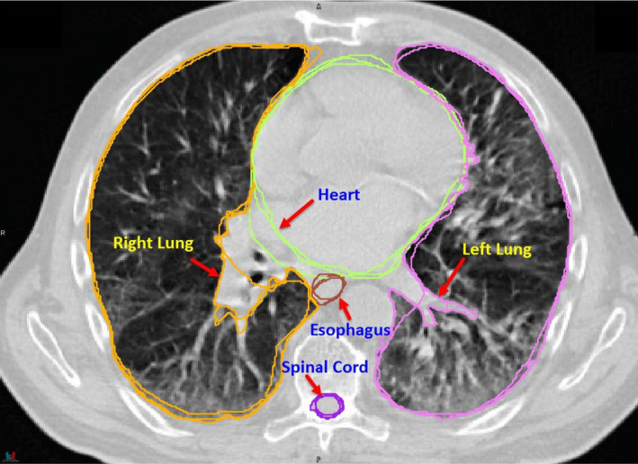
The following organs at risk (OARs) are used in this challenge: esophagus, heart, left and right lungs, and spinal cord (Fig. 1). The manual contours of these structures were drawn following the RTOG 1106 contouring atlas guideline,⁹ detailed as below.

Figure 1.

Organs used in the challenge: esophagus, heart, left and right lungs, and spinal cord. Bony structures are shown as the background. [Color figure can be viewed at wileyonlinelibrary.com]

Esophagus

RTOG 1106 description: The esophagus should be contoured from the beginning at the level just below the cricoid to its entrance to the stomach at GE junction. The esophagus will be contoured using mediastinal window/level on CT to correspond to the mucosal, submucosa, and all muscular layers out to the fatty adventitia.

Additional notes: The superior‐most slice of the esophagus is the slice below the first slice where the lamina of the cricoid cartilage is visible (±1 slice). The inferior‐most slice of the esophagus is the first slice (±1 slice) where the esophagus and stomach are joined, and at least 10 square cm of stomach cross section is visible.

Heart

RTOG 1106 description: The heart will be contoured along with the pericardial sac. The superior aspect (or base) will begin at the level of the inferior aspect of the pulmonary artery passing the midline and extend inferiorly to the apex of the heart.

Additional notes: Inferior vena cava is excluded or partly excluded starting at the slice where at least half of the vessel circumference is separated from the right atrium. Contouring of the pericardial sac remains inconsistent for some cases.

Lungs

RTOG 1106 description: Both lungs should be contoured using pulmonary windows. The right and left lungs can be contoured separately, but they should be considered as one structure for lung dosimetry. All inflated and collapsed, fibrotic and emphysematic lungs should be contoured; small vessels extending beyond the hilar regions should be included; however, gross tumor volume (GTV), hilars, and trachea/main bronchus should not be included in this structure.

Additional notes: Tumor is excluded in most data, but size and extent of excluded region are not guaranteed. Hilar airways and vessels greater than 5 mm (±2 mm) diameter are excluded. Main bronchi are always excluded, secondary bronchi may be included or excluded. Small vessels near hilum are not guaranteed to be excluded and were generally left as found in the original clinical contours. Collapsed lung may be excluded in some scans.

Spinal cord

RTOG 1106 description: The spinal cord will be contoured based on the bony limits of the spinal canal. The spinal cord should be contoured starting at the level just below cricoid (base of skull for apex tumors) and continuing on every CT slice to the bottom of L2. Neuroforamina should not be included.

Additional notes: Spinal cord may be contoured beyond cricoid superiorly and beyond L2 inferiorly. Contouring to base of skull is not guaranteed for apical tumors.

2.A.2. Quality assurance

The clinical contours from all institutions were quality checked prior to making data available, by one of the challenge organizers (GS), and edited to eliminate major deviations from RTOG 1106 contouring guidelines. For the lungs, images were edited to exclude main bronchi. In some cases, small vessels within lungs that were excluded in the original contours were edited to include them. The superior border of the heart was edited in some cases to comply with the RTOG guidelines. In some cases, the inferior and superior aspects of the esophagus and spinal cord were extended.

Prior to releasing the data, the challenge organizers discussed at length the degree to which data should be edited for quality assurance. Our consensus was that extensive editing of contouring was undesirable, because interobserver variability present in the original contours would be lost. For this reason, the data include several areas of inconsistency.

2.A.3. TCIA data curation

TCIA is a service for investigators who wish to share and download cancer imaging data for research purposes.⁸ The archive hosts data from a number of clinical trials and other NCI/NIH data collection initiatives but also allows the community to contribute datasets by filling out an application form.¹² After receiving approval to submit the dataset to TCIA, a quality check of all manual contours and CT images was performed. TCIA staff then provided customized versions of the Clinical Trial Processor software¹³ to deidentify and transfer the challenge dataset to TCIA servers. TCIA curators performed extensive review of both DICOM headers and pixel data to ensure full removal of patient identifiers in compliance with HIPAA regulations, while also taking care not to remove critical information necessary for analysis by challenge participants.¹⁴ The resulting dataset with detailed description can be obtained at http://doi.org/10.7937/K9/TCIA.2017.3r3fvz08.¹⁵

2.A.4. Interrater variability in the segmentation

Interrater variability refers to the variation in segmentation between multiple human operators. To be able to evaluate the automatic algorithms with respect to the interrater variability in human manual contouring, three cases were selected to be recontoured multiple times. The first training case from each of the contributing institutions was manually contoured by three of the authors (MG, GS, JY) according to the contouring guidelines. These additional contours were created without reference to the original contours submitted or to each other. Each quantitative measure used in the challenge was calculated pairwise between the three observers for each structure. Interrater variability was computed as the mean score between observers for each measure and for each organ and was used as a reference value to evaluate the performance of various algorithms for each structure.

2.B. Quantitative evaluation metrics

Submitted contours were compared against the manual contours, which serve as the ground truth, for all test datasets using the following evaluation metrics as implemented in Plastimatch.¹⁶ The RT structures were voxelized to CT resolution for all calculations which mean that accuracy evaluation is at the voxel level, and subvoxel differences between algorithms are not captured. Evaluation was performed in 3D. To prevent uncertainty with regard to the extent to which the spinal cord and esophagus should be contoured, both ground truth and submitted contours were cropped 1 cm superior to the inferior border, and 1 cm inferior to the superior border. Therefore, participants would not be penalized for contouring too great an extent of these structures in the inferior–superior direction, but would be penalized for a substantial undersegmentation.

2.B.1. Dice Coefficient

Dice coefficient is a measure of relative overlap, where 1 represents perfect agreement and 0 represents no overlap.

$$D=\frac{2X\cap Y}{+Y},$$ (1)

where X and Y are the ground truth and the submitted contours, respectively.

2.B.2. Mean surface distance (MSD)

The directed mean surface distance is the average distance of a point in X to its closest point in Y. That is:

$${\overrightarrow{d}}_{H,avg}(X,Y)=\frac{1}{}\sum _{x\in }\underset{y\in Y}{min}d\left(x,y\right)$$ (2)

The mean surface distance is the average of the two directed mean surface distances:

$$d_{H,avg}(X,Y)=\frac{{\overrightarrow{d}}_{H,avg}(X,Y)+{\overrightarrow{d}}_{H,avg}(Y,X)}{2}$$ (3)

2.B.3. 95% Hausdorff distance (HD95)

The directed percent Hausdorff measure, for a percentile r, is the rth percentile distance over all distances from points in X to their closest point in Y. For example, the directed 95% Hausdorff distance is the point in X with distance to its closest point in Y greater or equal to exactly 95% of the other points in X. In mathematical terms, denoting the rth percentile as K _r , this is given as:

$${\overrightarrow{d}}_{H,r}(X,Y)=K_r\left(\underset{y\in Y}{min}d\left(x,y\right)\right)\forall x\in X$$ (4)

The (undirected) percent Hausdorff measure is defined again with the mean:

$$d_{H,r}(X,Y)=\frac{{\overrightarrow{d}}_{H,r}(X,Y)+{\overrightarrow{d}}_{H,r}\left(Y,X\right)}{2}$$ (5)

2.B.4. Score normalization

Different organs and measures have different ranges of scores for the three metrics; therefore, it is not meaningful to average them to get an overall score. Thus, the scores were normalized with respect to interrater variability values generated from the three cases contoured by multiple raters. The mean score of these raters was used as a reference measure against which submitted contours were compared. For any organ/metric, a perfect value was given a score of 100. A value equivalent to the mean interrater reference was given a score of 50. A linear scale was be used to interpolate between these values, and extrapolate beyond them, such that a score of 0 was given to any result below the reference by more than the perfect score is above the reference. Mathematically,

$$\text{score}=max\left(\left(50+\frac{(T-R)}{(P-R)}\times 50\right),0\right)$$ (6)

where T is the test contour measure, P is the perfect measure (Dice = 1, MSD/HD95 = 0), and R is the reference measure for that organ/measure. For example, given a reference Dice of 0.85; a test contour with a Dice of 0.9 against the “ground truth" will score 66.6, where as a test contour with a Dice of 0.72 against the “ground truth" would score 7. Overall score of each participant was computed by averaging over all metrics, all structures, and all patients.

2.C. Algorithms used in online contest

We reported both offline and online competition results from seven teams who participated in both contests. A brief description of the segmentation algorithm used by each team is presented as below with a summary of these methods shown in Table 1.

Table 1.

Summary of specific implementation details of various segmentation methods used in the contest. Testing time is the segmentation time for one patient. DLC, deep‐learning contouring; MAC, multi‐atlas contouring

Method	Approach	Unique implementation features	Training time	Testing time	Run‐time GPU
1	DLC	• Hierarchical segmentation: use lung to constrain location of other structures	3 days	30 s	Titan X 12GB
		• 2.5D (lung) and 3D (others) residual Unets
		• Training from scratch
2	DLC	• Two‐step segmentation: first step to locate structures and second step to segment structures	2 days	10 s	Titan Xp 12GB
		• 3D Unet
		• Separate networks trained for each structure
3	DLC	• 2D Multiclass network to reduce the demand for a high spec graphics card at run time	>7 days	6 min	GTx 1050 2GB
		• Fine tuning of pretrained network
		• Loss function penalizing small structures
4	MAC	• Structure‐specific label fusion	–	8 h	–
5	DLC	• 2D ResNet	14 days	2 min	K40
		• Fine tuning of pretrained network
		• Use uncurated and unpreprocessed training data from an operating clinic; no postprocessing
6	MAC	• Organ‐based STAPLE fusion	–	5 min	–
7	DLC	• 3D (lung, heart) and 2D(others) Unets	4 h	2 min	Pascal
		• Google Inception layers for convolution

2.C.1. Method 1 — Team Elekta

This approach used a deep‐convolutional neural network (DCNN) for thoracic CT image segmentation. The DCNN model was modified from the U‐Net architecture,¹⁷ with 27 convolutional layers in total and with the sequential convolutional layers at each resolution level being combined into a residual block.¹⁸ To improve computation efficiency, two models were trained and applied in sequence. A fast 2.5D model with an input size of 5 × 360 × 360 voxels was trained to segment the lungs, the results of which were also used to automatically define a bounding box for the other structures. A 3D model with an input size of 32 × 128 × 128 voxels was trained and applied within the smaller ROI to get the final segmentation of the heart, the esophagus, and the spinal cord. The models were implemented using the Caffe package¹⁹ and trained from scratch using the 36 AAPM training datasets.

2.C.2. Method 2 — Team University of Virginia

This method used a two‐step deep‐learning model based on 3D U‐Net for thoracic segmentation. Preprocessing included intensity normalization and image resizing to unify pixel spacing and slice thickness. In the first step, a 3D U‐Net model was trained to segment all ROIs from downsampled images. The network structure contained three encoding layers and three decoding layers based on VGGNet²⁰ and the weighted cross entropy was used as the loss function. Bounding boxes for each ROI were then extracted as the input for the second step and one network is trained per ROI to segment background and foreground pixels. The final contours were cleaned to remove small nonconnected regions in automatic postprocessing.

2.C.3. Method 3 — Team Mirada

This approach employed convolutional networks to learn features in the input images that can be used to generate a dense (semantic) segmentation. A 2D multiclass network with 14 layers was first used to predict all OARs at a coarse resolution. The weighting of the loss function for the different classes was set empirically to favor smaller structures to improve their accuracy. The output of the initial network together with the full‐resolution image data formed the inputs to a series of organ‐specific ten‐layer networks that performed binary classification for each organ. Connected components and hole filling were used to correct discontinuities in the final segmentation. The networks were trained using the 36 training cases provided to refine the parameters that had been previously trained on 450 clinical patient cases. The network architectures were designed so that the processing of test cases could be carried out on a GPU with 2GB of RAM. Training was performed using a 8GB GPU.

2.C.4. Method 4 — Team University of Minho

A multi‐atlas segmentation approach with two conceptual steps, namely registration and label fusion, was applied.²¹ Concerning the registration step, for each atlas, after an initial full‐image alignment, each organ was independently masked and aligned through an affine model. Next, the affine transformations of individual organs were fused into a single transformation using a dense deformation field reconstruction strategy, guaranteeing the spatial coherence among organs. Next, a full nonrigid image registration was applied to refine the atlas to the patient anatomy. Concerning the label fusion step, an initial statistical selection was performed. Here, for each organ, the Dice coefficient was used to compute the overlap between each atlas segmentation and a reference segmentation, that is, a local weighted sum of all segmentations based on the cross‐correlation between image/atlases.²² Next, the final segmentation was acquired by fusing the nine best‐ranked candidate segmentations using the joint label fusion strategy.²³

2.C.5. Method 5 — Team Beaumont

A fully automated deep‐learning approach was used, using a pretrained network previously developed for general OAR segmentation that was fine‐tuned on the provided training cases. Input was individual CT slices and voxel labels. A residual network design was used, with multiple downsampling steps. At each resolution level, deconvolution was used to upsample to input resolution. The resulting maps were summed to make the final voxel labels. The initial network was trained on 2867 plans approved for treatment. Preprocessing of input was an initial downsampling to half‐resolution and mean voxel subtraction. There was no significant postprocessing beyond upsampling.

2.C.6. Method 6 — Team Maastro

An organ‐based multi‐atlas segmentation (MABS) approach was developed by the Maastro Clinic Physics research team. First, a multistage deformable image registration algorithm calculated the affine and B‐spline deformation fields between all atlases and the patient with unknown contours. The obtained deformation fields were then applied on all atlas CT images and structures to calculate patient‐like geometries and structures. Bounding boxes around every organ were determined and used to crop the atlas and patient CT data. For every organ, the normalized cross‐correlation coefficient was calculated between all cropped deformed atlas CT images and the patient CT image. The highest scoring cropped atlas CT images were used as input for the simultaneous truth and performance level estimation (STAPLE) algorithm, which calculated the automatic generated contour that was smoothed in a final step. To segment the OARs of one patient, about 5 min of computing time was required using a 400 core HTCondor CPU cluster.

2.C.7. Method 7 — Team WUSTL

Depending on the size of the organs, two different U‐net networks¹⁷ were used. For larger organs like lung and heart, a 3D U‐net was used. In particular, the whole CT scan was downsampled to a size of 224 × 224 × 224 by 3D interpolation. The same size binary mask for each organ was used as output to the 3D U‐net. Due to the large size of the input, each group layer of the encoding branch of the U‐net had only one convolutional layer with a 3 × 3 × 3 kernel and the size of the input was reduced by half. Similarly, on the decoding, each layer had only one deconvolutional layer to double the size of the input that was then merged with the corresponding layer from the encoding. Although the architecture was simple, this approach worked surprisingly well for lung and heart due to the amount of information and the size of these organs. For the smaller organs like spinal cord and esophagus, a 2D U‐net was used. A patch of 224 × 224 pixels containing the organ was extracted from the original 512 × 512 image based on the location distribution of that organ in the training set. The 2D U‐net was modified from the original U‐Net¹⁷ by replacing the convolution layer with a Google Inception layer²⁴ to increase the ability of feature learning of the network. Both models were trained with the Dice coefficient as the loss function with Adam optimization, early stopping, and learning decay on a Nvidia Pascal GPU.

3. Results

3.A. Interrater variability in the segmentation

The interrater variabilities for three raters on three training cases for the various structures are summarized in Table 2. These numbers were used as the reference measure for score normalization. The qualitative differences among raters are shown in Fig. 2.

Table 2.

Interrater differences in segmentation of organs at risk (OARs) for the analyzed metrics. HD95, 95% Hausdorff distance; MSD, mean surface distance

OAR	Dice	HD95 (mm)	MSD (mm)
Lung left	0.956 ± 0.019	5.17 ± 2.73	1.51 ± 0.67
Lung right	0.955 ± 0.019	6.71 ± 3.91	1.87 ± 0.87
Heart	0.931 ± 0.015	6.42 ± 1.82	2.21 ± 0.59
Esophagus	0.818 ± 0.039	3.33 ± 0.90	1.07 ± 0.25
Spinal cord	0.862 ± 0.038	2.38 ± 0.39	0.88 ± 0.23

Figure 2.

Qualitative display of interrater differences in segmentation of organs at risk. [Color figure can be viewed at wileyonlinelibrary.com]

3.B. Challenge results

The overall scores achieved by the seven methods are summarized in Fig. 3. Overall scores were computed by averaging the normalized scores over all measures, all structures, and all patients as described in subsection “Score normalization” of Section 2.B..

Figure 3.

Overall scores for each method for both offline and online evaluations. Box plots are generated from 12 offline and online test cases, respectively. Dots in the box are the mean scores of each method. A score of 50 is equivalent to average interrater variation. [Color figure can be viewed at wileyonlinelibrary.com]

Segmentation results for each organ, metric, and method for the online challenge are summarized in Figs. 4, 5, 6, 7 and Table 3. In general, the deep‐learning methods outperformed the multi‐atlas‐based methods. There was little difference in the performance among the various methods, namely, deep learning or atlas‐based, on generating a segmentation for large structures such as the lungs; larger performance differences were evident for narrow and long structures with poor soft‐tissue contrast such as the esophagus. It is interesting to note that both multi‐atlas methods, Method 4 and Method 6, slightly outperformed Method 5 and Method 7, both of which were deep‐learning algorithms for segmenting esophagus. Figure 8 shows an example segmentation generated by each method. The overall score achieved by those methods for segmenting the various structures is also shown. Referring to Fig. 7, it can be seen that performance of the methods varies according to the image on which assessment is performed. For example, in case LCTSC‐Test‐S2‐203, there is substantial tumor burden at the edge of the right lung. All methods perform uncharacteristically poorly for this organ in this case, highlighting impact of how the tumor is treated by such autocontouring methods.

Figure 4.

The Dice values achieved by the seven methods for the evaluated organs in the online contest. The reference Dice value computed from the interrater variability in manual segmentation, for which the normalized score is 50, is shown as the dashed line. (a) left and right lungs; (b) heart; (c) spinal cord; and (d) esophagus. [Color figure can be viewed at wileyonlinelibrary.com]

Figure 5.

The 95% Hausdorff distance (HD95) achieved by the seven methods for the evaluated organs in the online contest. The reference HD95 value computed from the interrater variability in manual segmentation, for which the normalized score is 50, is shown as the dashed line. (a) left and right lungs; (b) heart; (c) spinal cord; and (d) esophagus. NOTE: In plot (c), method 3 has an outlier of 5.3 mm that does not show within the plot area. [Color figure can be viewed at wileyonlinelibrary.com]

Figure 6.

The mean surface distance (MSD) achieved by the seven methods for the evaluated organs in the online contest. The reference MSD value computed from the interrater variability in manual segmentation, for which the normalized score is 50, is shown as the dashed line. (a) left and right lungs; (b) heart; (c) spinal cord; and (d) esophagus. [Color figure can be viewed at wileyonlinelibrary.com]

Figure 7.

The normalized score, averaged over all organs reported by CT for the online test data. [Color figure can be viewed at wileyonlinelibrary.com]

Table 3.

Segmentation performance of the seven methods for the evaluated organs in the online contest. The results are expressed as mean ± standard deviation for metrics including Dice coefficient, 95% Hausdorff distance (HD95), and mean surface distance (MSD)

Metric	Method	Organ
		Left lung	Right lung	Heart	Esophagus	Spinal cord
Dice	1	0.97 ± 0.02	0.97 ± 0.02	0.93 ± 0.02	0.72 ± 0.10	0.88 ± 0.037
	2	0.98 ± 0.01	0.97 ± 0.02	0.92 ± 0.02	0.64 ± 0.20	0.89 ± 0.042
	3	0.98 ± 0.02	0.97 ± 0.02	0.91 ± 0.02	0.71 ± 0.12	0.87 ± 0.110
	4	0.97 ± 0.01	0.97 ± 0.02	0.90 ± 0.03	0.64 ± 0.11	0.88 ± 0.045
	5	0.96 ± 0.03	0.95 ± 0.05	0.92 ± 0.02	0.61 ± 0.11	0.85 ± 0.035
	6	0.96 ± 0.01	0.96 ± 0.02	0.90 ± 0.02	0.58 ± 0.11	0.87 ± 0.022
	7	0.95 ± 0.03	0.96 ± 0.02	0.85 ± 0.04	0.55 ± 0.20	0.83 ± 0.080
HD95 (mm)	1	2.9 ± 1.32	4.7 ± 2.50	5.8 ± 1.98	7.3 ± 10.31	2.0 ± 0.37
	2	2.2 ± 0.79	3.6 ± 2.30	7.1 ± 3.73	19.7 ± 25.90	1.9 ± 0.49
	3	2.3 ± 1.30	3.7 ± 2.08	9.0 ± 4.29	7.8 ± 8.17	2.0 ± 1.15
	4	3.0 ± 1.08	4.6 ± 3.45	9.9 ± 4.16	6.8 ± 3.93	2.0 ± 0.62
	5	7.8 ± 19.13	14.5 ± 34.4	8.8 ± 5.31	8.0 ± 3.80	2.3 ± 0.50
	6	4.5 ± 1.62	5.6 ± 3.16	9.2 ± 3.10	8.6 ± 3.82	2.1 ± 0.35
	7	4.4 ± 3.41	4.1 ± 2.11	13.8 ± 5.49	37.0 ± 26.88	8.1 ± 10.72
MSD (mm)	1	0.74 ± 0.31	1.08 ± 0.54	2.05 ± 0.62	2.23 ± 2.82	0.73 ± 0.21
	2	0.61 ± 0.26	0.93 ± 0.53	2.42 ± 0.82	6.30 ± 9.08	0.69 ± 0.25
	3	0.62 ± 0.35	0.91 ± 0.52	2.89 ± 0.93	2.08 ± 1.94	0.76 ± 0.60
	4	0.79 ± 0.27	1.06 ± 0.63	3.00 ± 0.96	2.03 ± 1.94	0.71 ± 0.25
	5	2.90 ± 6.94	2.70 ± 4.84	2.61 ± 0.69	2.48 ± 1.15	1.03 ± 0.84
	6	1.16 ± 0.43	1.39 ± 0.61	3.15 ± 0.85	2.63 ± 1.03	0.78 ± 0.14
	7	1.22 ± 0.61	1.13 ± 0.49	4.55 ± 1.59	13.10 ± 10.39	2.10 ± 2.49

Figure 8.

Example segmentations generated by the seven methods for the organs under evaluation (left and right lungs, heart, esophagus, and spinal cord) shown in axial, sagittal, and coronal views. First row shows the manual contours. The overall score achieved by each method in segmenting these structures for this example patient is also shown. [Color figure can be viewed at wileyonlinelibrary.com]

Offline performance of the methods was similar to their online performance with the deep‐learning methods outperforming the multi‐atlas‐based methods (with the exception of slice‐based Unet in Method 7). Detailed results were provided in Data S1 (ChallengeResults.xlsx).

4. Discussion

4.A. Findings of the challenge

The results of this challenge follow a similar pattern to that found in many other computer‐assisted tasks; deep learning appears to outperform established methods. Atlas‐based autocontouring could be considered the established method for the task of automatic contouring of OARs, with the majority of vendors using this approach in their clinically available products.²⁵ However, the highest placed atlas‐based method in the challenge came in fourth place, with the top three entries all using deep‐learning contouring (DLC).

Specific implementation differences among the various methods is summarized in Table 1. On average, the DLC methods were computationally faster than the multi‐atlas contouring despite differences in the hardware. The slowest DLC method is from Team 3 that used a GTx 1050 2GB GPU, which can certainly achieve much faster segmentation with a faster GPU, and the fastest DLC is the Method 2 (around 10 s on a Titan Xp GPU). It is interesting to note that Method 1 did training from scratch as opposed to all other DLC methods but yet achieved the best results possibly due to the hierarchical segmentation approach where the lung segmentation was used to reduce the search space for the remaining structures. Methods 2 and 3 used multiscale approach to locate the structures followed by refining the segmentation of those structures within the detected regions.

Many of the DLC methods were based on variations U‐net architectures. The architecture modifications included residual connections used in the Unet (Method 1), VGG‐net layers used for convolutional layers (Method 2), and Google Inception layers used for performing convolutions in the 2D Unets (Method 7). While all methods opted to use a two‐step approach, with initial coarse segmentation being performed prior to a higher resolution refinement, variations exist how this was done and the dimensionality (with 2D, 3D, and 2.5D all represented) of the layers. However, analysis of the impact of architecture alone is not possible from the results of the challenge, since the method of training also differed with some using only the challenge data, and others pretraining on alternative data first.

It is worth noting that DLC is not guaranteed to be better; Method 7 did not perform as well as more conventional approaches. As with all methods, there are better and worse implementations, and deep learning in this context is a new and evolving technology. Furthermore, there were no participants who submitted results using shape models, a method that demonstrated high accuracy in the 2015 head and neck challenge.⁷

One possible explanation of why DLC outperforms atlas‐based segmentation comes from the greater number of degrees of freedom with DLC. Assuming a dense deformation registration for single atlas contouring, it can be expected that there are three degrees of freedom per CT image voxel. Therefore for the typical image size in this challenge (512 × 512 × 150), such a single atlas contouring method would have approximately 120 million degrees of freedom. However, voxels related to the structures to be contoured are a small portion of the entire image. In addition, in practice, deformable image registration is regularized to prevent unrealistic deformation and often constrained to a deformation model to make the solution computationally tractable. Thus, even if there is apparently one vector per voxel, they are constrained to behave in a dependent fashion such that the relative anatomical location of the object is preserved, and the effective number of degrees of freedom is substantially reduced in practice. In contrast, DLC has many more degrees of freedom, with Methods 1, 2, and 3 reporting approximately 27 million, 66 million, and 14 million free parameters in their models, respectively. Therefore, DLC should be able to capture more anatomical variation than atlas‐based contouring with its many more degrees of freedom. It should be noted that the results‐focused nature of this challenge means that this explanation remains a conjecture that has not been fully researched.

4.B. Implications for clinical practice

Following the online challenge results presentation at AAPM, a round table discussion considered implications in clinical practice. The discussion focused on three key aspects: the utility of such challenges for informing clinical practice, the adoption of autocontouring into clinical practice, and the open challenges in autocontouring for the future.

4.B.1. Are challenges useful for informing clinical practice?

Assessment of autocontouring within the context of a challenge must be quantitative; the challenge seeks to rank participating approaches in an objective fashion. To this end, quantitative measures such as Dice and Hausdorff distance as a gold standard are used. However, it has been observed that there is only weak correlation between such quantitative assessment and the editing time required to adapt contours to a clinically acceptable standard,²⁶ and this quantitative assessment is more affected by interobserver agreement.²⁷ While alternative qualitative assessment approaches have been proposed to overcome this limitation,^{28, 29, 30} such methods do not lend themselves to the challenge scenario. This raises the question as to whether such challenges are useful to inform clinical practice.

While not fully informing the resultant impact on clinical practice, such quantitative assessment is a useful gatekeeper prior to clinical impact investigation. To properly investigate the clinical impact through editing studies will require clinical time, and clinical time is a valuable commodity. Performing such an investigation on a poorly performing method is a waste of effort and risks alienating clinical staff against future investigation. Therefore, it is better to prove new approaches in such a quantitative comparison prior to clinical investigation, both as risk mitigation against wasting clinical effort and as a motivation tool for participating clinicians.

A noted limitation of such challenges is the limited pool of data and its restriction to “typical” cases. Although a single case with a partially collapsed lung was included in this challenge, poorly acquired and extreme pathological cases were excluded. Would it be fair to compare methods for their ability to segment a lung that is not present in a case where it had been surgically removed? What should be considered the right answer in such a context? However, autocontouring systems must be robust to such cases in a clinical context. While it is trivial to delete a structure returned for an organ that is not present in the image, such an abnormality may also impact the contouring quality of other organs that are present. In future challenges, it would be useful to consider this scenario with a broader range of training and test cases. Careful consideration would need to be given to assessing performance of methods according to the degree of abnormality to avoid biasing the overall conclusion to a single pathological case.

4.B.2. What limits use of autocontouring in clinical practice?

Commercial autocontouring systems have been available for 10 yr. However, in an audience poll at AAMD 2017, while approximately 80% of clinical institutions reported having autocontouring systems, only about 30% routinely use them. Anecdotally, the discontinued use may be attributed to two principal reasons: poor quality of results and poor workflow integration.

While current available model‐based and atlas‐based systems have been shown to reduce contouring time in clinical studies^{31, 32, 33, 34, 35, 36}, such studies often exclude cases with large abnormalities. Thus, although time may be saved in routine clinical practice for many cases, even a moderate number of “failure” cases that require more time to edit than would be required for manual contouring can lead to frustration and discontinuation of use by the clinical end user.

Some existing solutions may suffer from poor workflow integration; any additional demands on clinical users to navigate menus, to select, or to wait for autocontouring can be perceived as an additional time burden compared with manual contouring that outweighs any perceived benefit. Furthermore, most manual contouring tools are better suited to initial manual contouring than they are to editing of autogenerated structures. This, in turn, can lead to a poor perception of autocontouring, even if it is the editing tools that are the limiting factor.

4.B.3. Future directions for autocontouring

The drawbacks limiting the use in clinical practice naturally highlight potential directions for autocontouring research. Autocontouring challenges, such as this one, do not reward “I don’t know” as an answer. Users may prefer a system that does not return a contour where it has low confidence and indicates where manual intervention is most likely to be required. Future challenges should consider integrating the level of confidence into the scoring system or the automated detection of slices for editing. If some amount of manual editing is to be accepted as necessary, then there is also potential for innovation around the manual editing of existing structures in a more efficient manner. Evaluating and comparing such manual tools in an unbiased way present a challenge of its own.

While the majority of contouring for radiotherapy is currently performed on CT imaging, the increasing use of MRI is on the horizon. MRI presents an additional challenge for autocontouring. Autocontouring systems would need to adapt to variations in acquisition between institutions or even between different patients.

4.C. Limitations of the challenge

Although the challenge largely succeeded in bringing together researchers to discuss and learn about the state of the art in autocontouring on thoracic CT, there were technical limitations in the data and methods that should be considered when interpreting the results.

The total size of the data was limited to 60 subjects, split between training and evaluation. Given the dependence of machine learning approaches on a broad dataset, it is possible that some of the methods would have been able to perform even better with a larger data pool. However, arranging a large well‐curated dataset is difficult and perhaps a limitation of these approaches.

Although an attempt was made to clearly define a contouring standard for the challenge, various aspects of the scoring of the autocontouring may have unfairly penalized some of the methods in the evaluation. The evaluation of left and right lungs was based on the clinical judgment of the boundaries between healthy lung and tumor. Methods that extended the contour into the target volume were penalized, despite the fact that this could be easily excluded by a Boolean operation after segmentation. Also for the lungs, it was hard to ensure consistency in the exclusion or inclusion of small vessels in the ground truth data. Additionally, the patient inclusion/exclusion criteria were not firmly defined, for example, the collapsed lung and esophageal extent were based on visual judgment instead.

The challenge also was limited in how it can be interpreted in a clinical context. Several structures of clinical interest were not evaluated, such as brachial plexus, heart chambers, coronary vessels, and bronchial tree. Furthermore, the relationship between the quantitative measures used in the challenge and their normalized summary scores has not been clearly demonstrated to correlate well with clinical utility.

5. Conclusions

The 2017 AAPM Thoracic Auto‐Segmentation Challenge provided a standardized dataset and evaluation platform for testing and discussing the state‐of‐the art automatic segmentation methods for radiotherapy. The benchmarking datasets were made available to the public through TCIA¹⁵ and the evaluation platform was made available at our challenge website.¹¹ In line with current trends, we observed that deep‐learning approaches outperformed the multi‐atlas segmentation approaches. Roundtable discussion identified lack of good segmentation validation tools integrated into the clinical workflow as a main limiting factor for clinical implementation of autosegmentation methods and suggested segmentation self‐evaluation as a possible solution for clinical integration.

Supporting information

Data S1. Details of the competition results of 2017 AAPM thoracic auto‐segmentation grand challenge.

References

- 1. Ezzell GA, Galvin JM, Low D, et al. Guidance document on delivery, treatment planning, and clinical implementation of IMRT: report of the IMRT subcommittee of the AAPM radiation therapy committee. Med Phys. 2003;30:2089–2115. [DOI] [PubMed] [Google Scholar]
- 2. Mackie TR, Kapatoes J, Ruchala K, et al. Image guidance for precise conformal radiotherapy. Int J Radiat Oncol Biol Phys. 2003;56:89–105. [DOI] [PubMed] [Google Scholar]
- 3. Stapleford LJ, Lawson JD, Perkins C, et al. Evaluation of automatic atlas‐based lymph node segmentation for head‐and‐neck cancer. Int J Radiat Oncol Biol Phys. 2010;77:959–966. [DOI] [PubMed] [Google Scholar]
- 4. Yang J, Wei C, Zhang L, Zhang Y, Blum RS, Dong L. A statistical modeling approach for evaluating auto‐segmentation methods for image‐guided radiotherapy. Comput Med Imaging Graph. 2012;36:492–500. [DOI] [PMC free article] [PubMed] [Google Scholar]
- 5. Pekar V, Allaire S, Kim J, Jaffray DA. Head and neck auto‐segmentation challenge. MIDAS J. 2009;11. [Google Scholar]
- 6. Pekar V, Allaire S, Qazi AA, Kim JJ, Jaffray DA. Head and neck auto‐segmentation challenge: segmentation of the parotid glands. In: Medical Image Computing and Computer Assisted Intervention (MICCAI). Beijing; 2010:273–280. [Google Scholar]
- 7. Raudaschl PF, Zaffino P, Sharp GC, et al. Evaluation of segmentation methods on head and neck CT: auto‐segmentation challenge 2015. Med Phys. 2017;44:2020–2036. [DOI] [PubMed] [Google Scholar]
- 8. Clark K, Vendt B, Smith K, et al. The Cancer Imaging Archive (TCIA): maintaining and operating a public information repository. J Digit Imaging. 2013;26:1045–1057. [DOI] [PMC free article] [PubMed] [Google Scholar]
- 9. Kong F. Randomized phase II trial of individualized adaptive radiotherapy using during‐treatment FDG‐PET/CT and modern technology in locally advanced non‐small cell lung cancer (NSCLC) (1/26/16); 2016.
- 10. Kong F‐MS, Ritter T, Quint DJ, et al. Consideration of dose limits for organs at risk of thoracic radiotherapy: Atlas for lung, proximal bronchial tree, esophagus, spinal cord, ribs, and brachial plexus. Int J Radiat Oncol Biol Phys. 2011;81:1442–1457. [DOI] [PMC free article] [PubMed] [Google Scholar]
- 11. AAPM Thoracic Auto‐segmentation Challenge . http://autocontouringchallenge.org. Accessed September 1, 2018.
- 12. The Cancer Imaging Archive . Primary data. http://www.cancerimagingarchive.net/primary-data/. Accessed September 1, 2018.
- 13. RSNA Clinical Trials Processor (CTP) . https://www.rsna.org/ctp.aspx. Accessed September 1, 2018.
- 14. Moore SM, Maffitt DR, Smith KE, et al. De‐identification of medical images with retention of scientific research value. RadioGraphics. 2015;35:727–735. [DOI] [PMC free article] [PubMed] [Google Scholar]
- 15. Yang J, Sharp G, Veeraraghavan H, et al. Data from lung CT segmentation challenge. Cancer Imaging Arch. 2017. [Google Scholar]
- 16. Plastimatch . http://plastimatch.org. Accessed September 1, 2018.
- 17. Ronneberger O, Fischer P, Brox T. U‐net: convolutional networks for biomedical image segmentation. In: International Conference on Medical Image Computing and Computer‐Assisted Intervention. Berlin: Springer; 2015:234–241. [Google Scholar]
- 18. He K, Zhang X, Ren S, Sun J. Deep residual learning for image recognition. In: Proceedings of the IEEE Conference on Computer Vision and Pattern Recognition. Las Vegas, NV: IEEE; 2016:770–778. [Google Scholar]
- 19. Jia Y, Shelhamer E, Donahue J, et al. Caffe: convolutional architecture for fast feature embedding. In: Proceedings of the 22nd ACM International Conference on Multimedia. Orlando, FL: ACM; 2014:675–678. [Google Scholar]
- 20. Simonyan K, Zisserman A. Very deep convolutional networks for large‐scale image recognition. arXiv preprint arXiv:1409.1556; 2014.
- 21. Oliveira B, Queirós S, Morais P, et al. A novel multi‐atlas strategy with dense deformation field reconstruction for abdominal and thoracic multi‐organ segmentation from computed tomography. Med Image Anal. 2018;45:108–120. [DOI] [PubMed] [Google Scholar]
- 22. Artaechevarria X, Munoz‐Barrutia A, Ortiz‐de Solórzano C. Combination strategies in multi‐atlas image segmentation: application to brain MR data. IEEE Trans Med Imaging. 2009;28:1266–1277. [DOI] [PubMed] [Google Scholar]
- 23. Wang H, Suh JW, Das SR, Pluta JB, Craige C, Yushkevich PA. Multi‐atlas segmentation with joint label fusion. IEEE Trans Pattern Anal Mach Intell. 2013;35:611–623. [DOI] [PMC free article] [PubMed] [Google Scholar]
- 24. Szegedy C, Liu W, Jia Y, et al. Going deeper with convolutions. In: Proceedings of the IEEE Conference on Computer Vision and Pattern Recognition. Boston, MA: IEEE; 2015:1–9. [Google Scholar]
- 25. Sharp G, Fritscher KD, Pekar V, et al. Vision 20/20: perspectives on automated image segmentation for radiotherapy. Med Phys. 2014;41. [DOI] [PMC free article] [PubMed] [Google Scholar]
- 26. Gautam A, Weiss E, Williamson J, et al. SU‐C‐WAB‐03: assessing the correlation between quantitative measures of contour variability and physician's qualitative measure for clinical usefulness of auto‐segmentation in prostate cancer radiotherapy. Med Phys. 2013;40:90. [Google Scholar]
- 27. Langmack K, Perry C, Sinstead C, Mills J, Saunders D. The utility of atlas‐assisted segmentation in the male pelvis is dependent on the interobserver agreement of the structures segmented. Br J Radiol. 2014;87:20140299. [DOI] [PMC free article] [PubMed] [Google Scholar]
- 28. Greenham S, Dean J, Fu CKK, et al. Evaluation of atlas‐based auto‐segmentation software in prostate cancer patients. J Med Radiat Sci. 2014;61:151–158. [DOI] [PMC free article] [PubMed] [Google Scholar]
- 29. Gooding M, Chu K, Conibear J, et al. Multicenter clinical assessment of dir atlas‐based autocontouring. Int J Radiat Oncol Biol Phys. 2013;87:S714–S715. [Google Scholar]
- 30. Lustberg T, van Soest J, Gooding M, et al. Clinical evaluation of atlas and deep learning based automatic contouring for lung cancer. Radiother Oncol. 2018;126:312–317. [DOI] [PubMed] [Google Scholar]
- 31. La Macchia M, Fellin F, Amichetti M, et al. Systematic evaluation of three different commercial software solutions for automatic segmentation for adaptive therapy in head‐and‐neck, prostate and pleural cancer. Radiat Oncol. 2012;7:160. [DOI] [PMC free article] [PubMed] [Google Scholar]
- 32. Daisne JF, Blumhofer A. Atlas‐based automatic segmentation of head and neck organs at risk and nodal target volumes: a clinical validation. Radiat Oncol. 2013;8:154. [DOI] [PMC free article] [PubMed] [Google Scholar]
- 33. Langmack KA, Perry C, Sinstead C, Mills J, Saunders D. The utility of atlas‐assisted segmentation in the male pelvis is dependent on the interobserver agreement of the structures segmented. Br J Radiol. 2014;87:20140299. [DOI] [PMC free article] [PubMed] [Google Scholar]
- 34. Walker GV, Awan M, Tao R, et al. Prospective randomized double‐blind study of atlas‐based organ‐at‐risk autosegmentation‐assisted radiation planning in head and neck cancer. Radiother Oncol. 2014;112:321–325. [DOI] [PMC free article] [PubMed] [Google Scholar]
- 35. Eldesoky AR, Yates ES, Nyeng TB, et al. Internal and external validation of an ESTRO delineation guideline – dependent automated segmentation tool for loco‐regional radiation therapy of early breast cancer. Radiother Oncol. 2016;121:424–430. [DOI] [PubMed] [Google Scholar]
- 36. Yang J, Haas B, Fang R, et al. Atlas ranking and selection for automatic segmentation of the esophagus from CT scans. Phys Med Biol. 2017;62:9140–9158. [DOI] [PMC free article] [PubMed] [Google Scholar]
Associated Data
This section collects any data citations, data availability statements, or supplementary materials included in this article.
Supplementary Materials