Benchmarking Metagenomics Tools for Taxonomic Classification

Summary

Metagenomic sequencing is revolutionizing the detection and characterization of microbial species, and a wide variety of software tools are available to perform taxonomic classification of this data. The fast pace of development of these tools, alongside the complexity of metagenomic data, make it important that researchers are able to benchmark their performance. Here, we review current approaches for metagenomic analysis and evaluate the performance of 20 metagenomic classifiers using simulated and experimental datasets. We describe the key metrics used to assess performance, offer a framework for the comparison of additional classifiers, and discuss the future of metagenomic data analysis.

Identifying the microbial taxon or taxa present in complex biological and environmental samples is one of the oldest and most frequent challenges in microbiology, from determining the etiology of an infection from a patient’s blood sample to surveying the bacteria in an environmental soil sample (Jones et al., 2017; Pedersen et al., 2016; Somasekar et al., 2017; Zhang et al., 2016). Prior to the advent of genomic sequencing technologies, identifying taxa required time-consuming sequential testing of candidates (Pavia, 2011; Venkatesan et al., 2013). The application of metagenomic sequencing is transforming microbiology by directly interrogating the community composition in an unbiased manner, enabling more rapid species detection, the discovery of novel species and reducing reliance on culture-dependent approaches (Knights et al., 2011; Loman et al., 2013). The potential application of these technologies to improve diagnostics and in public health settings has also been widely recognized (Chiu and Miller, 2019; Miller et al., 2013), and there is extensive ongoing work to overcome the challenges associated with clinical use of these approaches (Blauwkamp et al., 2019; Miller et al., 2019).

As metagenomic sequencing produces genomic data from a set of species instead of a pure species isolate, one of the primary challenges in the field is the development of computational methods for identifying all of the species contained in these samples (Figure 1). There are two primary drivers of this computational challenge. Firstly, the widespread use of high throughput sequencing technologies that generate millions of short sequences (generally 50 – 200nt), presents a computational challenge for classifying large numbers of reads in a reasonable time. BLAST (basic local alignment and search tool) is one of the most well-known and commonly used software programs for DNA search and alignment against a database of genomic sequences (Altschul et al., 1990). Although BLAST is one of the most sensitive metagenomics alignment methods, it is computationally intensive, making it infeasible to run on the millions of reads typically generated by metagenomic sequencing studies. Secondly, this challenge is compounded by the exponential growth in recent years in the number of sequenced microbial genomes, meaning that the number of comparisons that need to be performed for new sequencing reads is huge and ever-increasing.

Figure 1.

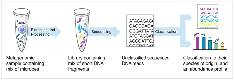
Processing steps to go from a complex metagenomic sample to an abundance profile of sample content

Many software tools have recently been developed to taxonomically classify metagenomic data and estimate taxa abundance profiles. For accurate analysis and interpretation of this data it is important to understand both how these different tools, broadly referred to as classifiers, work and how to determine the best approach for a given sample type, microbial kingdom or application. This includes continually benchmarking the ensemble of tools for the best performance characteristics along multiple dimensions: classification accuracy, speed, and computational requirements. Several groups have previously benchmarked metagenomic tools (Lindgreen et al., 2016; Mavromatis et al., 2007; McIntyre et al., 2017; Meyer et al., 2019; Sczyrba et al., 2017), but the continual introduction of newer tools requires ongoing evaluation to compare them against established tools. Here we review the core principles of metagenomic sequence classification methods, describe how to evaluate classifier performance and use these approaches to benchmark 20 commonly used taxonomic classifiers. To account for database differences and updates between methods, we further compare the performance of these tools on a uniform database, which has not been considered in earlier studies. We also provide recommendations for their use and describe future directions for the expansion of this field.

Efficient classification of millions of reads

A large number of tools have recently been developed that are focused on classifying large amounts of sequencing reads to known taxa with increasing speed. These taxonomic classifiers require pre-computed databases of previously sequenced microbial genetic sequences against which sequencing data is matched.

Within taxonomic classifiers a distinction can be made between taxonomic binning and taxonomic profiling. Binning approaches provide classification of individual sequence reads to reference taxa. Profilers report the relative abundances of taxa within a dataset but do not classify individual reads. However, in practice, these methods are often used interchangeably in analysing metagenomic sequencing data. Although not generated by default, a taxonomic profile can be calculated from binning approaches by summing up the individual read classifications. Taxonomic classifiers should not be confused with a distinct class of assembly-based tools for analysis of metagenomic sequencing data that cluster contigs de novo without the aid of any reference databases, an approach known as reference-free binning (Alneberg et al., 2014; Kang et al., 2015; Wu et al., 2016). These tools cannot taxonomically classify sequences and thus are not evaluated here, but have recently been benchmarked elsewhere (Sczyrba et al., 2017).

To generate assignments, classifiers utilize newer algorithmic approaches to ensure that classification speeds are fast enough for even large numbers of sequencing reads. To do so, most tools first seek to reduce the number of candidate hits for processing via approaches such as searching for stretches of perfect sequence matches with reference sequences (k-mers, typically around 31 nucleotides in length) or via an FM-index (Ferragina and Manzini, 2000). As a result, these methods are typically not as sensitive as BLAST, but are designed to be much faster. In addition, they frequently favor more memory usage to reduce CPU usage, and thus classification time. These tools can be divided into three groups: DNA to DNA classification (BLASTn-like), DNA to protein (BLASTx-like) classification, and marker-based classification.

DNA to DNA and DNA to protein tools classify sequencing reads by comparison to comprehensive genomic databases of DNA or protein sequences, respectively. DNA to protein tools are more computationally intensive than DNA to DNA tools because they need to analyze all six frames of potential DNA to amino acid translation, but they can be more sensitive to novel and highly variable sequences due to the lower mutation rates of amino acid compared to nucleotide sequences (Altschul et al., 1990). DNA to protein tools, however, target only the coding sequence of the genome, and therefore will not be able to classify non-coding sequencing reads as a result.

Marker-based methods typically include in their reference database only a subset of gene sequences instead of whole genomes, normally specific gene families that have good discriminatory power between species. The most widely used single marker gene for bacterial metagenomics is the highly conserved 16S rRNA sequence (Edgar, 2018; Yarza et al., 2014), though other markers are needed to identify viruses, fungi and other microbes that do not have the 16S marker gene. Some marker-based methods, such as MetaPhlAn2, address this limitation by indexing a number of different gene families in its database to identify taxa from other microbial kingdoms (Truong et al., 2015). The use of a subset of genes makes these methods quick, however, the marker sequences used can introduce a bias in the results if they are not evenly distributed among the microbial sequences of interest (D’Amore et al., 2016).

Size and growth of reference databases

All metagenomics classifiers require a pre-computed database based on previously sequenced microbial genetic sequences, whose sheer size presents a considerable computational challenge. The most popular reference databases are RefSeq complete genomes for microbial species, as well as the BLAST nt and nr databases for high-quality nucleotide and protein sequences from all kingdoms of life with ~50 and ~200 million sequences respectively as of 2019. Other databases include SILVA for 16S rRNA (ribosomal RNA) with ~2 million sequences and Genbank for a larger quantity of genomes with lower quality control standards (Benson et al., 2005; Quast et al., 2013).

The universe of microbial sequences is very diverse and these resulting databases are fairly large, typically requiring 10–100s of gigabytes. This vast search space can also result in a significant number of false positive classifications because of the large number of possible taxa against which the sequences are matched. Additionally, the large universe of presently undiscovered microbial species can result in false negative classifications simply because the genetic sequences have never been categorized in a database before. Recent efforts to expand the number of known microbial genomes have highlighted the improvement in the proportion of reads classified compared to older databases (Forster et al., 2019), but must be balanced with the challenges of handling larger databases.

All classifier tools are distributed with pre-compiled reference databases, the composition of which can vary substantially between classifiers. This can act as a confounder in comparing the classification performance across methods. These databases may use entirely different sources for sequence data, or, even if they share a common source for sequences (e.g. RefSeq), continual updates and addition of new sequences will mean databases created at different times will have different content. Most tools also allow a user to build their own database based on a desired set of sequences. This is a computationally intensive process, especially for comprehensive databases, but affords the user greater control over the analysis — especially when investigating rare, recently discovered or highly diverse species. Given the complexity of both the test samples and reference databases in metagenomic classification, it is further important to perform comparisons using a uniform database to eliminate any confounding effects of differences in default database compositions.

Comparing classifier performance

The metrics selected to benchmark classifiers can greatly influence their relative rankings and performance and thus must be carefully selected to best reflect the way these tools are used in practice. The most important metrics for metagenomic classification are precision and recall. Precision is the proportion of true positive species identified in the sample divided by the number of total species identified by the method, while recall is defined as the proportion of true positive species divided by the number of distinct species actually in the sample. These measures, and derived metrics, are commonly used across benchmarking studies (McIntyre et al., 2017; Meyer et al., 2019; Sczyrba et al., 2017). The F1 score is the harmonic mean of recall and precision, weighting them equally in a single metric. However, as end-users will often filter out taxa below a certain abundance threshold, using a single raw precision, recall, or F1 score does not provide a realistic estimate of classifier performance.

To better assess precision and recall scores across all abundance thresholds, it is preferable to use a precision-recall curve, where each point represents the precision and recall scores at a specific abundance threshold (Figure 2). By ranging the abundance threshold from 0–1.0, the area under this precision-recall curve (AUPR) outputs a single metric to aggregate precision and recall scores (Davis and Goadrich, 2006; Saito and Rehmsmeier, 2015). It should be noted that precision and recall focus only on the positive class of identified taxa. Performance metrics that require the calculation of false negatives, such as ROC curves, are less informative in this context because false negatives are poorly defined in real-world metagenomic samples. A potential drawback of AUPR is that it is biased towards low precision, high recall classifiers. Classifiers that don’t recall all of the ground truth taxa are penalized with zero AUPR from the highest achieved recall to 100% recall. For classifiers that do reach 100% recall, additional false positive taxa calls do not further penalize the AUPR score.

Figure 2.

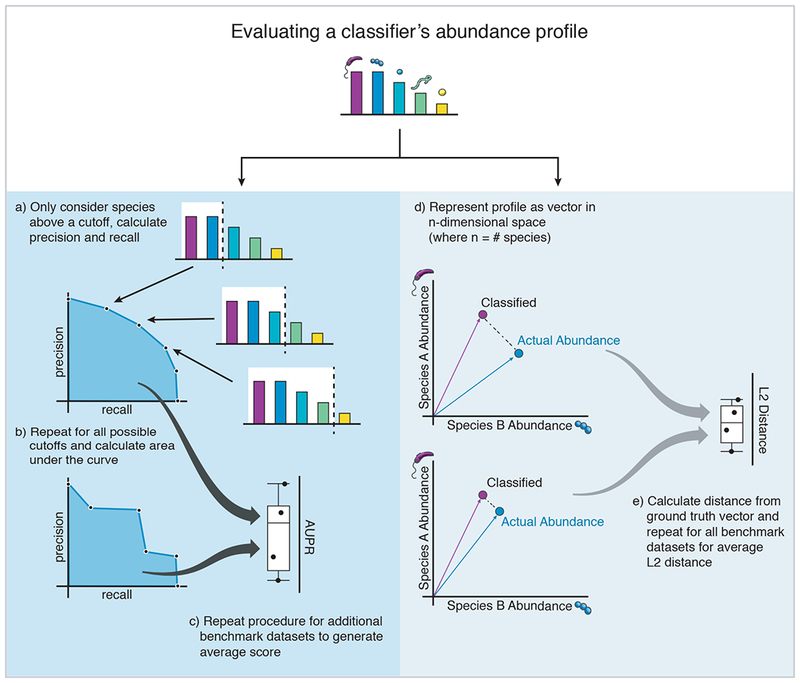
Metrics used for evaluating classifier performance. AUPR and L2 distance are two complementary metrics that provide insight into the accuracy of a classifiers precision/recall and abundance estimates, respectively. Considered together they provide a readily interpretable picture of classifier performance and can be used to compare between classifiers.

In addition to considering the number of correctly identified species, it is also important to evaluate how accurately the abundance of each species or genera in the resulting classification reflects the abundance of each species in the original biological sample (“ground truth”). This is especially critical for applications such as microbiome sequencing studies where changes in population composition can confer phenotypic effects (Morgan et al., 2012; Ross et al., 2013). Abundance can be considered either as the relative abundance of reads from each taxa (“raw”) or by inferring abundance of the number of individuals from each taxa by correcting read counts for genome size (“corrected”). Some programs incorporate a correction for genome length into abundance estimates, or this calculation can also be manually performed by reweighting the read counts after classification. Here we use raw abundance profiles unless correction is performed automatically by the software, as in the case of PathSeq and Bracken.

To evaluate the accuracy of abundance profiles we can calculate the pairwise distances between ground truth abundances and normalized abundance counts for each identified taxa at a given taxonomic level (e.g. species or genus). For this we calculate the L2 distance for a given dataset’s classified output as the straight-line distance between the observed and true abundance vectors (Figure 2). We can also use this measure to compare abundance profiles between classifiers by instead computing L2 distances between classified abundances for pairs of classifiers. Abundance profile distance is more sensitive to accurate quantification of the highly abundant taxa present in the sample (Aitchison, 1982; Quinn et al., 2018). High numbers of very low abundance false positives will not dramatically affect the measure as they comprise only a small portion of the total abundance. For this reason, using such a measure alongside AUPR, which is highly sensitive to classifiers’ performance in correctly identifying low-abundance taxa, allows for a comprehensive evaluation of classifier performance.

The L2 distance should be considered as a representation of the abundance profiles. Since metagenomic abundance profiles are proportional data and not absolute data, it is important to remember that many common distance metrics (including L2 distance) are not true mathematical metrics in proportional space (Badri et al., 2018; Quinn et al., 2018). Generally in proportional data analysis, a common method is to normalize proportions by using the centered log-ratio transform to calculate distances. However, the output of these metagenomic classifiers include many low-abundance false positives leading to sparse zero counts for many taxa across the different reports. The log-transform of these zero counts is undefined unless arbitrary pseudocounts are added to each taxa, which can negatively bias accurate classifiers because false positive taxa will have added counts. Another commonly used metric to compare abundance profiles is the UniFrac distance, which considers both the abundance proportion of component taxa, as well as the evolutionary distance for incorrectly called taxa (Lozupone and Knight, 2005). However, using this metric is complicated by the difficulty in assessing evolutionary distance between microbial species’ whole genomes.

Metrics should also be tested across many datasets as classifiers may perform better or worse on certain species or sample types. Lastly, other features — such as classification speed, memory usage and output format — may also influence the choice of classifier and should also be considered in any thorough evaluation.

Evaluating the precision-recall of 20 classifiers

Here we benchmarked 20 metagenomic classifiers to compare performance in classification precision, recall, F1, speed, and other metrics using a uniform database to eliminate any confounding effects of differences in default databases. DNA to DNA classifiers evaluated here were Kraken (and its add-on for more accurate abundance quantification Bracken), Kraken2, KrakenUniq, k-SLAM, MegaBLAST, metaOthello, CLARK, CLARK-S, GOTTCHA, taxMaps, prophyle, PathSeq, Centrifuge, and Karp. DNA to Protein classifiers evaluated were DIAMOND, Kaiju, and MMseqs2. We also evaluate the marker-based methods MetaPhlAn2 and mOTUs2. A more detailed description of each classifier’s qualitative characteristics is provided in Table 1 and Supplementary Table 1. To evaluate classifier performance controlling for database differences, a uniform database was created when possible based on RefSeq complete microbial genomes (RefSeqCG) and benchmarked for each method alongside the default database. We considered the precision and recall across a range of abundance thresholds as well as overall abundance profiles as our primary benchmarking metrics.

Table 1.

A list of benchmarked classifiers and their various characteristics. Custom databases refers to the ability for the end user to create a custom database. The time and memory requirements are for a 5.7 million read dataset with the database and input already cached in memory. Some methods (marked as “varies”) have the ability to flexibly decrease their memory usage (at the cost of massive increase in runtime).

Type	Classifier	Custom Databases	Generates Abundance Profile	Memory Required	Time Required	Reference
DNA	Bracken	Yes	Yes	< 1 Gb	< 1 min	(Lu et al., 2017)
	Centrifuge	Yes	Yes	20 Gb	7 min	(Kim et al., 2016)
	CLARK	Yes	Yes	80 Gb	2 min	(Ounit et al., 2015)
	CLARK-S	Yes	Yes	170 Gb	40 min	(Ounit and Lonardi, 2016)
	Kraken	Yes	Yes	190 Gb	1 min	(Wood and Salzberg, 2014)
	Kraken2	Yes	Yes	36 Gb	1 min	(Wood and Salzberg, 2014)
	KrakenUniq	Yes	Yes	200 Gb	1 min	(Breitwieser et al., 2018)
	k-SLAM	Yes	Yes	130 Gb	2 hr	(Ainsworth et al., 2017)
	MegaBLAST	Yes	No	61 Gb	4 hr	(Morgulis et al., 2008)
	metaOthello	No	No	30 Gb	1 min	(Liu et al., 2018)
	PathSeq	Yes*	No	140 Gb	5 min	(Walker et al., 2018)
	prophyle	Yes	No	40 Gb	40 min	(Břinda et al., 2017)
	taxMaps	Yes	Yes	65 Gb	25 min	(Corvelo et al., 2018)
Protein	DIAMOND	Yes	No	110 Gb (varies)	10 min	(Buchfink et al., 2015)
	Kaiju	Yes	Yes	25 Gb	1 min	(Menzel et al., 2016)
	MMseqs2	Yes	No	85 Gb (varies)	9 hr	(Steinegger and Söding, 2017)
Markers	MetaPhlAn2	No	Yes	2 Gb	1 min	(Truong et al., 2015)
	mOTUs2	No	Yes	2 Gb	1 min	(Milanese et al., 2019)

^*The latest version of PathSeq now allows the user to create and specify a custom database but this option was not available when benchmarking studies were performed thus it was excluded from those analyses.

To first evaluate the precision and recall of each method we ran all 20 classifiers using a set of 10 benchmarking datasets composed of computationally simulated reads from between 12 and 525 bacterial species (see Supplemental Information) and generated a report of identified taxa and their corresponding abundance proportions within the sample. Each classifier was run using default parameters with the exception of adding mild filtering for MegaBLAST and Kraken (see Supplemental Information). Output reports were then reformatted to allow for comparison between classifiers at different taxonomic levels, and for each classifier report we calculated precision and recall (Figure S1), generated the precision-recall curve and computed the AUPR (Figure S2). Median AUPR was then calculated from the AUPR values of all datasets for a given classifier (as described in Figure 2).

Most methods performed well in terms of AUPR, with scores above 0.8 at the species level (Figure 3A) using their default databases. For most methods there is a gradual tradeoff between precision and recall as expected (Figure S2). Most of the performance falloff for AUPR came from a decline in precision at high recall. This is likely due to false positive taxa being classified at low abundance ahead of the lowest abundance true positive taxa. Genus-level performance tended to be slightly better than species-level classifications (Figure S3). In this study we do not consider classifications below species level. Sequence similarity between strains and other challenges mean it is generally preferred to use specialized approaches for accurate strain typing (Luo et al., 2015; Scholz et al., 2016; Truong et al., 2017).

Figure 3.

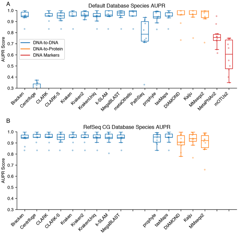
Benchmark AUPR Scores. A. Area under precision-recall curve (AUPR) scores for each classifier at the species level (higher value is better). Each plot point represents the score for a (classifier, dataset combination). Classifiers are grouped and colored by their target class. B. AUPR for the uniform RefSeq CG database instead of default databases. Missing entries on the RefSeq CG plot are classifiers that cannot create custom databases. For additional information see Figures S1–S4.

Two samples had notably low AUPR scores across multiple classifiers when using default databases. The buccal (oral microbiome) simulated dataset was a consistent low-scoring outlier among the DNA classifiers. This dataset is relatively small and only contains 12 different species, of which one species, Neisseria subflava, was a contig-quality assembly. This lower quality assembly is not included in most DNA databases but is in the nr database. The simulated ATCC Staggered dataset was a consistently poor performing sample for the protein-based classifiers because it contains taxa at very low abundances, making false positive classifications more likely especially when using the expansive nr database.

Database limitations negatively affect a few classifiers: MetaPhlAn2 and mOTUs2, with limited marker-based databases, naturally had lower performance. Centrifuge’s default database is significantly lossily compressed (throwing away database sequences to save space), which also results in poor recall. Karp’s recommended database of microbial rRNA sequences is too limited to perform well, and it would be unfair to draw further conclusions from its much smaller database. We additionally excluded GOTTCHA as it has known L2 abundance estimation biases (McIntyre et al., 2017). Additional benchmarking results for GOTTCHA and Karp are available in Supplemental Figures S1–S6, but otherwise they were excluded from further analysis.

To evaluate the importance of the reference database in taxonomic classifications, we constructed databases for each method from a normalized set of microbial RefSeq complete genomes from the archaea, bacteria, and viral kingdoms. To create the corresponding protein-based databases, we used the protein sequences of these complete genomes. This custom standardized database is referred to as RefSeq CG. We did not include fungal, protozoan, or other eukaryotic microbial genomes in RefSeq CG as these domains have relatively few complete genomes. Not all methods supported custom database construction (Table 1) so those classifiers could not be assessed. Overall, classifiers’ AUPR scores on the RefSeq CG databases were slightly worse than on their own default databases (Figure 3B), with the difference being most pronounced for the protein-based methods. The protein coding subset of RefSeq CG is both smaller than the default nr protein databases, and smaller than theset of whole genomes indexed by DNA classifiers. For many of the DNA classifiers, the performance between classifiers was much more similar using the RefSeq CG database than with their own databases, indicating that these methods behave fairly similarly. Inherent database differences contributed more variation to the performance differences between DNA classifiers. Centrifuge’s score improved because the Refseq CG database was not lossily compressed, in contrast to the default compressed database.

To more thoroughly test the impact of poorly characterized, divergent, and novel sequences on classification, we additionally evaluated performance on the Critical Assessment of Metagenome Interpretation (CAMI) datasets (Sczyrba et al., 2017) (see Supplemental Information). While these datasets are also simulated based on short DNA sequencing reads, they are comprised of dramatically different taxa profiles. For these datasets, only ~30–40% of reads are simulated from known taxa, whereas the rest of the reads are from novel taxa, plasmids or simulated evolved strains. The AUPR of the CAMI samples was very low at the species rank, while performance improved significantly at the genus classification rank (Figure S4). This is due to the small numbers of taxa for which there is a ground truth specified at the species rank, as well as the confounding effects of large quantities of sequences from unknown taxa, which is also confirmed by the low classified abundances (Figure S5). Performance was also broadly similar between classifiers of each class, and became even more similar when using the normalized RefSeq CG databases.

Comparing abundance profile distances for 20 classifiers

We next evaluated the accuracy of the estimated abundance profiles across classifiers compared to the ground truth. For those methods that did not directly output an abundance profile (Table 1), this was calculated as described in the Supplemental Information. We then calculated the L2 distance between classified and true abundances of all species (see Figure 4), and considered the average L2 distance across all datasets for a classifier as representative of the accuracy of that classifier.

Figure 4.

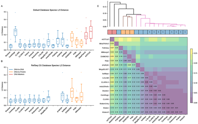
Benchmark L2 Distances A. Distance between the species abundance profile for each classifier compared to the true composition (lower value is better). Each plot point represents the L2 distance for a (classifier, dataset) combination. Classifiers are grouped and colored by their target class. B. Abundance distance using the uniform RefSeq CG database. Missing entries are those classifiers that cannot create custom databases C. Median pairwise L2 abundance norms between classifiers across simulated datasets, hierarchically clustered. Non-black cluster link colors are groups at a 0.09 similarity threshold. Colored boxes correspond to the method type: DNA, Protein, and Marker classifiers. The ‘k’ annotation indicates k-mer based methods. For additional information see Figure S6.

DNA based classifiers that used long k-mers (> 30 nt), such as Kraken and taxMaps, were among the best scoring methods with typical average L2 distances from the truth below 0.1 (Figure 4A). The marker-based and, to a lesser extent, protein classifiers had higher L2 distances, demonstrating that they performed less well (Figure 4A). Genus abundance distances were generally lower than species abundance distances (Figure S6). Additionally, using the standardized database of Refseq CG did not change abundance distances much compared to default databases (Figure 4B), with the notable exception of Centrifuge which again improved dramatically when used with a database that is not lossily compressed. Notably, Bracken - a post-processing step intended to improve abundance estimates by Kraken - does provide more accurate abundances at the species level (Figure 4A & Figure S6). This step is a simple and worthwhile addition to Kraken for better abundance estimates.

To assess the similarities of the classifiers between each other, we performed a hierarchical clustering using the median L2 distances calculated between pairs of classifiers across all datasets. The k-mer based methods cluster very closely together with MegaBLAST and prophyle falling slightly outside of the tight main cluster (Figure 4C). The protein classifiers cluster together although their profiles are quite different from each other. As expected, marker-based methods MetaPhlAn2 and mOTUs2 have abundances estimates that are very different to both DNA and protein classifiers. PathSeq is very divergent from other DNA methods. This may be because reads matching multiple taxa cannot be disambiguated and thus may be counted multiple times. It also internally corrects the taxa abundance by genome lengths, whereas we evaluate based on raw read abundance.

The AUPR and abundance profile distances only consider the classified proportion of each sample. These metrics do not assess the proportion of reads left unclassified, or those classified to a very broad taxonomy node, such as “All Bacteria”, which are less informative in describing the sample composition. Classifiers vary greatly in the proportion of reads they classified at the species rank (Figure 5). Classified proportions further varied greatly between sample datasets with the same classifier. Protein classifiers had many more unclassified reads, as is expected, due to the databases only containing coding regions of the genome. It should be noted that Bracken, although measured as having the highest proportion of reads classified, does not actually classify the reads directly. Instead, it reassigns the unclassified proportion based on probabilistic estimates of the true abundance profile from the original classified Kraken report.

Figure 5.

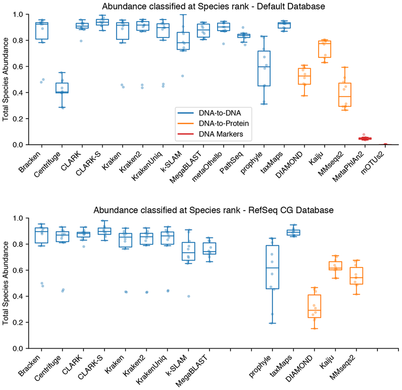
Proportion of abundance classified at the Species rank A. Proportion of sample abundance classified at the species rank with default databases. B. Using uniform RefSeq CG databases. Only programs allowing custom databases are shown in panel B. For additional information see Figure S5.

Determining the rate and source of false positive classifications

False positive classifications present a major challenge for the interpretation of metagenomic sequencing data, especially when considering human clinical samples (White et al., 2009). This can originate from several sources and could be influenced by experimental and analytical factors. At the classification stage, the absence of a species from the reference database can result in misclassification of reads from that species. The clearest example of this is host genomic content, especially as most default reference databases do not explicitly include the human genome. Using simulated genomic reads from the human hg38 reference genome we found that 1–5% of human reads were incorrectly classified for most DNA classifiers (Figure S7). Notably, classifiers that index the human genome in their default database, such as KrakenUniq and Centrifuge, had negligible rates of misclassification (Figure S7). The protein-based classifiers had higher misclassification rates, ranging from 5–15% misclassified abundance, partially due to the larger number of sequences in the default nr databases. Including known or suspected host genomes in a reference database is thus a first important step to reducing false positive classifications.

To distinguish incorrect classifications from contamination introduced during sample processing and sequencing, classifier outputs from simulated data were compared against sequencing data from real in vitro samples. We prepared and sequenced genomic DNA and total RNA from the ATCC Even, a metagenome standard containing 20 bacterial species each at 5% abundance, and compared it to the simulated DNA from the same standard (see Supplemental Information). For the simulated DNA, after the 20 ground truth species were recalled, additional false-positive species started appearing below 0.5% abundance for a few methods, while most classifiers called false-positives below the 0.01 % abundance (Figure 6 & Figure S8). The number of false positives ranged from tens (Bracken, MetaPhlAn2) to thousands (Centrifuge, CLARK, Kaiju, MMseqs2, PathSeq) of distinct species depending on the methods, although some methods levelled off at a certain abundance threshold, notably the marker-based methods, while others continued to call more and more false positives at lower abundances. These characteristics can be used to make an informed decision about the appropriate abundance level cut-off for post-filtering of classifications.

Figure 6.

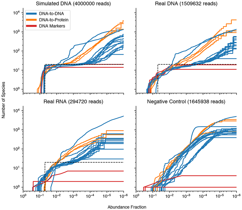
Number of species classified versus minimum abundance threshold detected in ATCC Even sample datasets. The truth abundance of 20 species at 0.05 abundance each is depicted as the black dotted line. For additional information see Figures S7–S9.

The problem of low abundance false positives is not captured well by the AUPR and abundance distance metrics. The AUPR curve concludes after the lowest abundance true positive is found, so further false positives do not decrease the AUPR score, while the total abundance sum of these false positives is small and doesn’t have much impact on L2 distance. Compared to the simulated DNA, the sequenced DNA exhibited a similar number and growth of false positives at lower abundances (Figure 6). This implies that false positive calls are mostly the result of computational false positives, instead of the sample degradation or contamination from working with wet-lab reagents and samples. In contrast, sequenced RNA tended to have faster false positive growth at higher abundances compared to the DNA datasets, making it more difficult to distinguish ground truth from incorrect species. This is probably due to the heavy bias of RNA content towards the highly conserved bacterial ribosomal RNA (rRNA) sequences, which by mass is typically much more abundant than mRNA in whole cells and are very similar between different bacterial species. However, the total number of false positives was typically lower than in DNA datasets, which is probably due to a shallower sequencing depth for the RNA samples making extremely low abundance species (~1 per million reads) stochastically disappear.

Abundance estimates were more inaccurate for the sequenced DNA and RNA datasets compared to simulated DNA (Figure 6 & S8). The microbiome standards initially contained an even 5% abundance for all 20 species, but the experimental protocols used to go from whole cell material to final sequencing reads likely biased the original abundances in a reproducible way. Steps such as PCR amplification tend to bias towards certain DNA library sequences, altering the original abundance compositions (Aird et al., 2011). Though the impact of PCR can be mitigated to some extent by removal of duplicate sequences this is not standard practice in most metagenomic classifiers. Additionally, a non-template control (NTC) was prepared and sequenced from ultrapure nucleic acid-free water. The NTC classifier reports also contained high numbers of false positives, unlike what would be expected for a completely clean sample containing no genetic material (Figure 6). It is important to note the NTC sample contained a significant amount of human DNA sequences that are likely the result of contamination (~70%), as measured by Kraken, but aside from human, most classifiers falsely classified less than 20% of the NTC abundance.

Compared to the simulated samples, the real life sequenced samples exhibited worse AUPR performance with a more significant decline for the total RNA samples (Figure S9). The protein and marker-based classifiers overall had more significant performance decreases compared to the DNA classifiers. Counterintuitively, the protein-based classifiers did markedly worse on the RNA samples. However, much of the RNA content from the total RNA is not mRNA coding for proteins but rather contains rRNA sequences which are not translated.

Another source of inaccuracy in most experimental protocols is PCR duplication, and removal of these duplicates is a challenge across classifiers. The NTC sample contained 75% duplicate reads, as compared to 15% for RNA and 0.01% for DNA as measured by cd-hit-dup. The high level of sequence duplication is expected for the NTC because it required a higher number of PCR amplification cycles to achieve the same DNA library concentrations as the real samples, however this is an issue for all amplified metagenomic samples. Most metagenomic classifiers do not remove these PCR duplicates as part of their classification, but this is an important step to generate more accurate abundance profiles, especially in cases where many cycles of amplification were performed as part of sample preparation.

Computational Requirements

The computational resources and time required for running a metagenomic classifier are varied and can be very high (Figure 7A & B). Apart from the marker-based methods, all of the classifiers used a significant amount of memory, which ranged from tens to hundreds of gigabytes. The marker-based methods also had the fastest initial classification time, using just a few minutes per million reads (Figure 7A). Among DNA-to-DNA classifiers, the FM-index and alignment methods typically used much less memory than those relying on large databases of long k-mers, however they had a higher runtime after database caching due to the pairwise alignments they perform. Interestingly, CLARK-S has a much higher runtime than CLARK even after database caching. without significantly improving accuracy. Among the DNA-to-protein classifiers, MMseqs2 required extremely high amounts of memory and computational time, while Kaiju was fairly quick due to the use of an FM-index. One reason for slow runtimes is that DNA-to-protein methods require querying six frame translations of the query DNA sequence, resulting in a significant increase in runtime compared to DNA methods, which becomes even more pronounced with increasing numbers of input sequences. These methods also typically use the more comprehensive BLAST nr database as their database, which includes proteins from non-microbial sources, whereas DNA-based classifiers tended to only incorporate microbial sequences.

Figure 7.

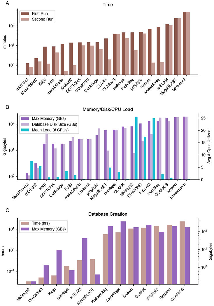
Benchmark of computational resources A. Time required to process a sample containing 5.7 million reads, versus a second run immediately after the first. This second run is faster for many classifiers because sample reads and database files are cached in memory. Bracken is not plotted as it requires negligible time/memory. B. The maximum memory utilized by each classifier during execution, the on-disk database size, and average number of cpus utilized out of 32 available. C. Time taken and memory used to create the RefSeq CG database using various methods. Classifiers are sorted by increasing time taken. MMseqs2 and DIAMOND don’t index the genomes during database construction, but rather index on-the-fly during sample classification.

A significant portion of the classification time may reflect the time required to load the reference database into memory. This is especially true of DIAMOND and MMseqs2, which do not index the database during creation but while the classification is actually performed, resulting in fast database creation but higher classification times. All other methods index the database during creation, which steeply increases the time required to create a database to several hours (Figure 7C) but reduces loading time each time a classification is performed.

Storage of the database in memory can reduce overall runtime when processing multiple samples. Some methods, such as Kraken and metaOthello, processed the second sample faster after loading the database into memory for the first sample (Figure 7A). Even though only CLARK(-S) explicitly supports batch-processing of multiple samples, consecutive back-to-back program executions mean that much of the database is still implicitly cached by the operating system and hasn’t been evicted from memory yet. However, not all methods improved during the second run, indicating that their databases were not cache friendly (Figure 7A). The disparity in runtime between a cached and uncached database can be up to 100x, so careful use of caching and batch processing can result in major performance improvements.

Discussion

Advancements in the field of metagenomic sequencing analysis have produced a suite of taxonomic classifiers that perform well across a range of datasets, meaning that other preferences or constraints should also guide method selection. The classifiers investigated here had similar performances, especially between classifiers of the same type, on the same dataset. Broadly, DNA classifiers provide better precision-recall and abundance estimates than protein-based classifiers when using a uniform database for these whole-genome datasets. This lower specificity of protein classifiers on the normalized RefSeq CG database can be largely attributed to the absence of non-coding sequence from their databases. Indeed, differences in default database compositions accounted for greater performance differences between classifiers than the methods themselves. This similarity in performance means that other factors such as the computational resources available, as well as the ease-of-use and other particulars of each classifier should be considered when deciding on the most appropriate tool.

The computational resource requirements of some programs may be prohibitive for some applications, so using classifiers that require lower memory incurs a tradeoff between computational cost and accuracy. Among DNA classifiers, when a server with high amounts of memory (>100 Gb) is available, Kraken and its derivative tools Bracken/KrakenUniq/Kraken2 provide good performance metrics, are very fast on large numbers of samples as long as the database loading time is amortized, and allow the creation and usage of custom databases. CLARK is a good alternative, however Kraken+Bracken tends to have slightly more accurate abundance profiles. If high amounts of memory are not available, MetaPhlAn2 is recommended for having very low computational requirements (<2Gb of memory), as well as fast classification speed but does not allow custom databases. If custom databases are desired, Centrifuge may be useful; it requires 10s of Gbs of memory and demonstrates good performance metrics, despite the shortcomings of the compressed default database. Among the protein-based classifiers, Kaiju is generally recommended for having much faster classification speed and lower memory requirements, compared to the other classifiers DIAMOND and MMseqs2, without compromising performance. All three of these methods allow custom databases.

Although most of the classifiers included in this study performed well across the benchmark datasets containing known taxa, there are several areas in which more development is needed to improve these tools. This includes both simple technical changes to existing methods as well as conceptual innovations in how these methods are used that could improve the quality of the results generated by these classifiers.

Classifiers perform very well when taxa in a sample are genetically distinct from each other and genetically similar to sequences in the reference database. Though not evaluated here, previous studies have shown that classification below the species level is challenging with current taxonomic classifiers (McIntyre et al., 2017; Sczyrba et al., 2017). The dramatically poorer performance of all classifiers on the CAMI datasets compared to the IMMSA datasets, further underlines the influence of evolutionary distance and poorly described taxa on classification performance. Relative classifier performance was largely consistent, indicating that these problems are common across existing tools. Expanding reference databases can improve classification (Forster et al., 2019), however, for datasets as divergent or complex as CAMI, where only a small proportion of abundance is able to be classified at the species or genus level (Figure S6), the taxa present are likely not known or very different to taxa in the reference database. De novo assembly of metagenomes may be a more appropriate strategy for analysis of such highly complex and novel metagenomic samples. These tools have recently identified thousands of novel metagenome assembled genomes in the human microbiome (Almeida et al., 2019; Nayfach et al., 2019; Pasolli et al., 2019)

One of the biggest performance challenges for many classifiers is that they often report large numbers of low abundance false positives, lowering the precision of these estimates. Most practitioners filter these reports using a given abundance threshold. Integration of this within software packages would improve classifier precision and standardisation and simplify downstream analyses. Another possibility for improving performance would be performing per-read filtering based on alignment score or e-value. Some classifiers have options that allow for this, but do not have default recommendations for using them. These values would depend on classifier support and would vary between classifiers and even experimental designs, which could make them difficult to use. In addition, practices such as including the mammalian / host genomes and potential contaminants in reference databases can help reduce misclassification due to missing reference sequences. The human genome is included in the default databases of several classifiers (Centrifuge, DIAMOND, Kaiju, KrakenUniq, MegaBLAST, MMseqs2) and can be included in a custom-built database with software that permit this. When the host is known, pre-filtering of host-derived sequences can also be used (Blauwkamp et al., 2019; Miller et al., 2019).

More generally, making full use of information available about sequenced reads - including incorporating sequence quality scores and PCR duplicate removal - common practices in other areas of sequence analysis, could further improve classification. Apart from Karp, most metagenomic methods don’t consider sequencer quality scores for classification. Using quality scores in a probabilistic context would increase the computational cost of classification, but could be a fruitful avenue for future research. Similarly, most classifiers generate profiles simply based on proportions of classified reads. Of the methods evaluated here, only Bracken takes a probabilistic approach to generate the final abundance profiles. Another common issue in low-input metagenomic sequencing is high PCR duplication rates of sequencing reads resulting from high numbers of PCR cycles. This can distort abundance estimates since certain taxa become dominant via high duplicate numbers. Some effort has been made by methods like KrakenUniq to estimate the unique nucleotide content of each taxa, to better determine duplication level and recover true abundances.

In addition to PCR duplication, there are a number of other features of the experimental preparation of samples for metagenomic sequencing that can confound classification performance. Cross-talk between multiplexed samples on Illumina flow-cells (especially notable on more recent sequencers that use patterned flow cells) can generate biological false positives at low abundances (Sinha et al., 2017). Library molecules can bleed through multiple runs on the sample sequencers. Samples can also pick up biological contamination from microbial sequences in the laboratory environment or genetic material present in extraction and library preparation reagents. These contaminants may confound benchmarking attempts using real sequenced datasets, however, this is part of a larger challenge of metagenomic classification that needs to be addressed. Specifically, while these are “true positives” from the perspective of the classifier as they were present in the final sequenced sample, they confound conclusions and inferences drawn from metagenomic classifiers. Clean laboratory practices as well as recent innovations to experimentally remove routine contaminants (Gu et al., 2016) or use artificial sequences to quantify contamination (Zinter et al., 2019) can reduce but are unlikely to be able to completely remove this problem.

The use of well-matched negative controls in any metagenomics study is essential to be able to identify and control for contamination. Though use of negative controls has recently improved in metagenomics studies, there is currently no accepted approach for correcting for contamination using these controls (Davis et al., 2018; McLaren et al., 2019). One interesting avenue for exploration is the use of negative control samples to create blacklists of known contaminants.

Thinking more broadly, one proposed strategy to address the individual shortcomings of different classifiers is to use an ensemble of classifiers, or a pipeline of different classifiers (McIntyre et al., 2017; Piro et al., 2017). For pipelines, typically a faster method is run first, while a slower but more sensitive method is run on the leftover unclassified or poorly classified reads (Bazinet et al., 2018; Jiang et al., 2017). This is sometimes performed in a more ad hoc fashion using protein classifiers as a second-pass analysis option for DNA classifiers because it offers higher sensitivity to mutations and more distantly related proteins, but trades lower specificity in response (Yang et al., 2014). The downside of ensemble classifiers is higher computational runtime and a more challenging interpretation of the results.

Runtime is a recurring challenge for many of these methods and though some methods use approaches that either reduce runtime or memory use, many classifiers have runtimes that are dictated by the disk speed of reading their databases into memory. After loading the database, classifying each incremental sample is extremely fast for methods such as Kraken and CLARK. Not all methods support classifying multiple samples in a single execution to explicitly take advantage of database caching, yet their database pages might by implicitly cached by the operating system for faster single-sample executions. Some methods such as DIAMOND and MMseqs2 perform large in-memory sorts that spill out temporary files on disk. These methods are faster with larger amounts of memory and fast temporary disks.

The rapid growth of reference databases will present a fundamental challenge to the field in coming years as this pace exceeds that of computer memories. This will likely create a number of secondary challenges that current software will need to adjust to. The growth of reference databases such as RefSeq can result in methods changing performance characteristics over time, as exemplified by the decrease in accuracy of k-mer based methods (Nasko et al., 2018). Many of these newly sequenced genomes are re-sequenced microbial strains that are very similar to existing species, resulting in oversampling of some genera and species groups. NCBI’s taxonomy database is frequently changing, with taxon nodes being constantly renamed, deleted, merged into other nodes, promoted and/or demoted from taxonomic ranks. There are some ways that software programs can mitigate taxonomy changes, such as including the full versioned taxonomy database tree for hosted pre-built metagenomic databases. However, these changes do not address the underlying challenge presented by the size and growth of these databases. Managing this data explosion is likely to be one of the biggest challenges in metagenomic sequence classification in the coming years and will require more wide-reaching changes in our approach.

The field of metagenomics is approaching a critical milestone in its trajectory. Investment in recent years has led to the development of a range of programs with good overall performance, giving users a choice of ways to analyse their data in accordance with their particular question, computational environment, target taxa and other preferences. This is making the analysis of metagenomic sequencing more accessible than ever before. However, many taxonomic classifiers are still burdened by high numbers of false positive calls at low abundance that need to be addressed. Looking beyond this, bigger breakthroughs will be needed in many areas, including in controlling experimental sources of contamination and error, and in handling the exponential growth of reference databases, in order to create transformational changes in metagenomic classification towards microbial detection and characterization.

References

- Ainsworth D, Sternberg MJE, Raczy C, and Butcher SA (2017). k-SLAM: accurate and ultra-fast taxonomic classification and gene identification for large metagenomic data sets. Nucleic Acids Res. 45, 1649–1656. [DOI] [PMC free article] [PubMed] [Google Scholar]
- Aird D, Ross MG, Chen W-S, Danielsson M, Fennell T, Russ C, Jaffe DB, Nusbaum C, and Gnirke A (2011). Analyzing and minimizing PCR amplification bias in Illumina sequencing libraries. Genome Biol. 12, R18. [DOI] [PMC free article] [PubMed] [Google Scholar]
- Aitchison J (1982). The Statistical Analysis of Compositional Data. J. R. Stat. Soc. Series B Stat. Methodol. 44, 139–177. [Google Scholar]
- Almeida A, Mitchell AL, Boland M, Forster SC, Gloor GB, Tarkowska A, Lawley TD, and Finn RD (2019). A new genomic blueprint of the human gut microbiota. Nature 568, 499–504. [DOI] [PMC free article] [PubMed] [Google Scholar]
- Alneberg J, Bjarnason BS, de Bruijn I, Schirmer M, Quick J, Ijaz UZ, Lahti L, Loman NJ, Andersson AF, and Quince C (2014). Binning metagenomic contigs by coverage and composition. Nat. Methods 11, 1144–1146. [DOI] [PubMed] [Google Scholar]
- Altschul SF, Gish W, Miller W, Myers EW, and Lipman DJ (1990). Basic local alignment search tool. J. Mol. Biol. 215, 403–410. [DOI] [PubMed] [Google Scholar]
- Badri M, Kurtz Z, Muller C, and Bonneau R (2018). Normalization methods for microbial abundance data strongly affect correlation estimates.
- Bazinet AL, Ondov BD, Sommer DD, and Ratnayake S (2018). BLAST-based validation of metagenomic sequence assignments. PeerJ 6, e4892. [DOI] [PMC free article] [PubMed] [Google Scholar]
- Benson DA, Karsch-Mizrachi I, Lipman DJ, Ostell J, and Wheeler DL (2005). GenBank. Nucleic Acids Res. 33, D34–D38. [DOI] [PMC free article] [PubMed] [Google Scholar]
- Blauwkamp TA, Thair S, Rosen MJ, Blair L, Lindner MS, Vilfan ID, Kawli T, Christians FC, Venkatasubrahmanyam S, Wall GD, et al. (2019). Analytical and clinical validation of a microbial cell-free DNA sequencing test for infectious disease. Nat Microbiol 4, 663–674. [DOI] [PubMed] [Google Scholar]
- Breitwieser FP, Baker DN, and Salzberg SL (2018). KrakenUniq: confident and fast metagenomics classification using unique k-mer counts. Genome Biol. 19, 198. [DOI] [PMC free article] [PubMed] [Google Scholar]
- Břinda K, Salikhov K, Pignotti S, and Kucherov G (2017). karel-Břinda/prophyle: ProPhyle 0.3.1.0.
- Buchfink B, Xie C, and Huson DH (2015). Fast and sensitive protein alignment using DIAMOND. Nat. Methods 12, 59–60. [DOI] [PubMed] [Google Scholar]
- Chiu CY, and Miller SA (2019). Clinical metagenomics. Nat. Rev. Genet. 20, 341–355. [DOI] [PMC free article] [PubMed] [Google Scholar]
- Corvelo A, Clarke WE, Robine N, and Zody MC (2018). taxMaps: Comprehensive and highly accurate taxonomic classification of short-read data in reasonable time. Genome Res. [DOI] [PMC free article] [PubMed] [Google Scholar]
- D’Amore R, Ijaz UZ, Schirmer M, Kenny JG, Gregory R, Darby AC, Shakya M, Podar M, Quince C, and Hall N (2016). A comprehensive benchmarking study of protocols and sequencing platforms for 16S rRNA community profiling. BMC Genomics 17, 55. [DOI] [PMC free article] [PubMed] [Google Scholar]
- Davis J, and Goadrich M (2006). The Relationship Between Precision-Recall and ROC Curves. In Proceedings of the 23rd International Conference on Machine Learning, (New York, NY, USA: ACM), pp. 233–240. [Google Scholar]
- Davis NM, Proctor DM, Holmes SP, Relman DA, and Callahan BJ (2018). Simple statistical identification and removal of contaminant sequences in marker-gene and metagenomics data. Microbiome 6, 226. [DOI] [PMC free article] [PubMed] [Google Scholar]
- Edgar RC (2018). Updating the 97% identity threshold for 16S ribosomal RNA OTUs. Bioinformatics 34, 2371–2375. [DOI] [PubMed] [Google Scholar]
- Ferragina P, and Manzini G (2000). Opportunistic Data Structures with Applications. In Proceedings of the 41st Annual Symposium on Foundations of Computer Science, (Washington, DC, USA: IEEE Computer Society), p. 390–398. [Google Scholar]
- Forster SC, Kumar N, Anonye BO, Almeida A, Viciani E, Stares MD, Dunn M, Mkandawire TT, Zhu A, Shao Y, et al. (2019). A human gut bacterial genome and culture collection for improved metagenomic analyses. Nat. Biotechnol. 37, 186–192. [DOI] [PMC free article] [PubMed] [Google Scholar]
- Gu W, Crawford ED, O’Donovan BD, Wilson MR, Chow ED, Retallack H, and DeRisi JL (2016). Depletion of Abundant Sequences by Hybridization (DASH): using Cas9 to remove unwanted high-abundance species in sequencing libraries and molecular counting applications. Genome Biol. 17, 41. [DOI] [PMC free article] [PubMed] [Google Scholar]
- Jiang Y, Wang J, Xia D, and Yu G (2017). EnSVMB: Metagenomics Fragments Classification using Ensemble SVM and BLAST. Sci. Rep. 7, 9440. [DOI] [PMC free article] [PubMed] [Google Scholar]
- Jones S, Baizan-Edge A, MacFarlane S, and Torrance L (2017). Viral Diagnostics in Plants Using Next Generation Sequencing: Computational Analysis in Practice. Front. Plant Sci. 8, 1770. [DOI] [PMC free article] [PubMed] [Google Scholar]
- Kang DD, Froula J, Egan R, and Wang Z (2015). MetaBAT, an efficient tool for accurately reconstructing single genomes from complex microbial communities. PeerJ 3, e1165. [DOI] [PMC free article] [PubMed] [Google Scholar]
- Kim D, Song L, Breitwieser FP, and Salzberg SL (2016). Centrifuge: rapid and sensitive classification of metagenomic sequences. Genome Res. 26, 1721–1729. [DOI] [PMC free article] [PubMed] [Google Scholar]
- Knights D, Kuczynski J, Charlson ES, Zaneveld J, Mozer MC, Collman RG, Bushman FD, Knight R, and Kelley ST (2011). Bayesian community-wide culture-independent microbial source tracking. Nat. Methods 8, 761–763. [DOI] [PMC free article] [PubMed] [Google Scholar]
- Lindgreen S, Adair KL, and Gardner PP (2016). An evaluation of the accuracy and speed of metagenome analysis tools. Sci. Rep. 6, 19233. [DOI] [PMC free article] [PubMed] [Google Scholar]
- Liu X, Yu Y, Liu J, Elliott CF, Qian C, and Liu J (2018). A novel data structure to support ultra-fast taxonomic classification of metagenomic sequences with k-mer signatures. Bioinformatics 34, 171–178. [DOI] [PMC free article] [PubMed] [Google Scholar]
- Loman NJ, Constantinidou C, Christner M, Rohde H, Chan JZ-M, Quick J, Weir JC, Quince C, Smith GP, Betley JR, et al. (2013). A culture-independent sequence-based metagenomics approach to the investigation of an outbreak of Shiga-toxigenic Escherichia coli O104:H4. JAMA 309, 1502–1510. [DOI] [PubMed] [Google Scholar]
- Lozupone C, and Knight R (2005). UniFrac: a new phylogenetic method for comparing microbial communities. Appl. Environ. Microbiol. 71, 8228–8235. [DOI] [PMC free article] [PubMed] [Google Scholar]
- Lu J, Breitwieser FP, Thielen P, and Salzberg SL (2017). Bracken: estimating species abundance in metagenomics data. PeerJ Comput. Sci. 3, e104. [Google Scholar]
- Luo C, Knight R, Siljander H, Knip M, Xavier RJ, and Gevers D (2015). ConStrains identifies microbial strains in metagenomic datasets. Nat. Biotechnol. 33, 1045–1052. [DOI] [PMC free article] [PubMed] [Google Scholar]
- Mavromatis K, Ivanova N, Barry K, Shapiro H, Goltsman E, McHardy AC, Rigoutsos I, Salamov A, Korzeniewski F, Land M, et al. (2007). Use of simulated data sets to evaluate the fidelity of metagenomic processing methods. Nat. Methods 4, 495–500. [DOI] [PubMed] [Google Scholar]
- McIntyre ABR, Ounit R, Afshinnekoo E, Prill RJ, Hénaff E, Alexander N, Minot SS, Danko D, Foox J, Ahsanuddin S, et al. (2017). Comprehensive benchmarking and ensemble approaches for metagenomic classifiers. Genome Biol. 18, 182. [DOI] [PMC free article] [PubMed] [Google Scholar]
- McLaren MR, Willis AD, and Callahan BJ (2019). Consistent and correctable bias in metagenomic sequencing measurements. [DOI] [PMC free article] [PubMed]
- Menzel P, Ng KL, and Krogh A (2016). Fast and sensitive taxonomic classification for metagenomics with Kaiju. Nat. Commun. 7, 11257. [DOI] [PMC free article] [PubMed] [Google Scholar]
- Meyer F, Bremges A, Belmann P, Janssen S, McHardy AC, and Koslicki D (2019). Assessing taxonomic metagenome profilers with OPAL. Genome Biol. 20, 51. [DOI] [PMC free article] [PubMed] [Google Scholar]
- Milanese A, Mende DR, Paoli L, Salazar G, Ruscheweyh H-J, Cuenca M, Hingamp P, Alves R, Costea PI., Coelho LP, et al. (2019). Microbial abundance, activity and population genomic profiling with mOTUs2. Nat. Commun. 10, 1014. [DOI] [PMC free article] [PubMed] [Google Scholar]
- Miller RR, Montoya V, Gardy JL, Patrick DM, and Tang P (2013). Metagenomics for pathogen detection in public health. Genome Med. 5, 81. [DOI] [PMC free article] [PubMed] [Google Scholar]
- Miller S, Naccache SN, Samayoa E, Messacar K, Arevalo S, Federman S, Stryke D, Pham E, Fung B, Bolosky WJ, et al. (2019). Laboratory validation of a clinical metagenomic sequencing assay for pathogen detection in cerebrospinal fluid. Genome Res. 29, 831–842. [DOI] [PMC free article] [PubMed] [Google Scholar]
- Morgan XC, Tickle TL, Sokol H, Gevers D, Devaney KL, Ward DV, Reyes JA, Shah SA, LeLeiko N, Snapper SB, et al. (2012). Dysfunction of the intestinal microbiome in inflammatory bowel disease and treatment. Genome Biol. 13, R79. [DOI] [PMC free article] [PubMed] [Google Scholar]
- Morgulis A, Coulouris G, Raytselis Y, Madden TL, Agarwala R, and Schaffer AA (2008). Database indexing for production MegaBLAST searches. Bioinformatics 24, 1757–1764. [DOI] [PMC free article] [PubMed] [Google Scholar]
- Nasko DJ, Koren S, Phillippy AM, and Treangen TJ (2018). RefSeq database growth influences the accuracy of k-mer-based species identification. [DOI] [PMC free article] [PubMed]
- Nayfach S, Shi ZJ, Seshadri R, Pollard KS, and Kyrpides NC (2019). New insights from uncultivated genomes of the global human gut microbiome. Nature 568, 505–510. [DOI] [PMC free article] [PubMed] [Google Scholar]
- Ounit R, and Lonardi S (2016). Higher classification sensitivity of short metagenomic reads with CLARK-S. Bioinformatics 32, 3823–3825. [DOI] [PubMed] [Google Scholar]
- Ounit R, Wanamaker S, Close TJ, and Lonardi S (2015). CLARK: fast and accurate classification of metagenomic and genomic sequences using discriminative k-mers. BMC Genomics 16, 236. [DOI] [PMC free article] [PubMed] [Google Scholar]
- Pasolli E, Asnicar F, Manara S, Zolfo M, Karcher N, Armanini F, Beghini F, Manghi P, Tett A, Ghensi P, et al. (2019). Extensive Unexplored Human Microbiome Diversity Revealed by Over 150,000 Genomes from Metagenomes Spanning Age, Geography, and Lifestyle. Cell 176, 649–662. e20. [DOI] [PMC free article] [PubMed] [Google Scholar]
- Pavia AT (2011). Viral infections of the lower respiratory tract: old viruses, new viruses, and the role of diagnosis. Clin. Infect. Dis. 52 Suppl 4, S284–S289. [DOI] [PMC free article] [PubMed] [Google Scholar]
- Pedersen HK, Gudmundsdottir V, Nielsen HB, Hyotylainen T, Nielsen T, Jensen BAH, Forslund K, Hildebrand F, Prifti E, Falony G, et al. (2016). Human gut microbes impact host serum metabolome and insulin sensitivity. Nature 535, 376–381. [DOI] [PubMed] [Google Scholar]
- Piro VC, Matschkowski M, and Renard BY (2017). MetaMeta: integrating metagenome analysis tools to improve taxonomic profiling. Microbiome 5, 101. [DOI] [PMC free article] [PubMed] [Google Scholar]
- Quast C, Pruesse E, Yilmaz P, Gerken J, Schweer T, Yarza P, Peplies J, and Glockner FO (2013). The SILVA ribosomal RNA gene database project: improved data processing and web-based tools. Nucleic Acids Res. 41, D590–D596. [DOI] [PMC free article] [PubMed] [Google Scholar]
- Quinn TP, Erb I, Richardson MF, and Crowley TM (2018). Understanding sequencing data as compositions: an outlook and review. Bioinformatics 34, 2870–2878. [DOI] [PMC free article] [PubMed] [Google Scholar]
- Ross EM, Moate PJ., Marett LC, Cocks BG, and Hayes BJ (2013). Metagenomic predictions: from microbiome to complex health and environmental phenotypes in humans and cattle. PLoS One 8, e73056. [DOI] [PMC free article] [PubMed] [Google Scholar]
- Saito T, and Rehmsmeier M (2015). The precision-recall plot is more informative than the ROC plot when evaluating binary classifiers on imbalanced datasets. PLoS One 10, e0118432. [DOI] [PMC free article] [PubMed] [Google Scholar]
- Scholz M, Ward DV, Pasolli E, Tolio T, Zolfo M, Asnicar F, Truong DT, Tett A, Morrow AL, and Segata N (2016). Strain-level microbial epidemiology and population genomics from shotgun metagenomics. Nat. Methods 13, 435–438. [DOI] [PubMed] [Google Scholar]
- Sczyrba A, Hofmann P, Belmann P, Koslicki D, Janssen S, Droge J, Gregor I, Majda S, Fiedler J, Dahms E, et al. (2017). Critical Assessment of Metagenome Interpretation-a benchmark of metagenomics software. Nat. Methods 14, 1063–1071. [DOI] [PMC free article] [PubMed] [Google Scholar]
- Sinha R, Stanley G, Gulati GS, Ezran C, Travaglini KJ, Wei E, Chan CKF, Nabhan AN, Su T, Morganti RM, et al. (2017). Index Switching Causes “Spreading-Of-Signal” Among Multiplexed Samples In Illumina HiSeq 4000 DNA Sequencing.
- Somasekar S, Lee D, Rule J, Naccache SN, Stone M, Busch MP, Sanders C, Lee WM, and Chiu CY (2017). Viral Surveillance in Serum Samples From Patients With Acute Liver Failure By Metagenomic Next-Generation Sequencing. Clin. Infect. Dis. 65, 1477–1485. [DOI] [PMC free article] [PubMed] [Google Scholar]
- Steinegger M, and Söding J (2017). MMseqs2 enables sensitive protein sequence searching for the analysis of massive data sets. Nat. Biotechnol. 35, 1026–1028. [DOI] [PubMed] [Google Scholar]
- Truong DT, Franzosa EA, Tickle TL, Scholz M, Weingart G, Pasolli E, Tett A, Huttenhower C, and Segata N (2015). MetaPhlAn2 for enhanced metagenomic taxonomic profiling. Nat. Methods 12, 902–903. [DOI] [PubMed] [Google Scholar]
- Truong DT, Tett A, Pasolli E, Huttenhower C, and Segata N (2017). Microbial strain-level population structure and genetic diversity from metagenomes. Genome Res. 27, 626–638. [DOI] [PMC free article] [PubMed] [Google Scholar]
- Venkatesan A, Tunkel AR, Bloch KC, Lauring AS, Sejvar J, Bitnun A, Stahl J-P, Mailles A, Drebot M, Rupprecht CE, et al. (2013). Case definitions, diagnostic algorithms, and priorities in encephalitis: consensus statement of the international encephalitis consortium. Clin. Infect. Dis. 57, 1114–1128. [DOI] [PMC free article] [PubMed] [Google Scholar]
- Walker MA, Pedamallu CS, Ojesina AI, Bullman S, Sharpe T, Whelan CW, and Meyerson M (2018). GATK PathSeq: a customizable computational tool for the discovery and identification of microbial sequences in libraries from eukaryotic hosts. Bioinformatics 34, 4287–4289. [DOI] [PMC free article] [PubMed] [Google Scholar]
- White JR, Nagarajan N, and Pop M (2009). Statistical methods for detecting differentially abundant features in clinical metagenomic samples. PLoS Comput. Biol. 5, e1000352. [DOI] [PMC free article] [PubMed] [Google Scholar]
- Wood DE, and Salzberg SL (2014). Kraken: ultrafast metagenomic sequence classification using exact alignments. Genome Biol. 15, R46. [DOI] [PMC free article] [PubMed] [Google Scholar]
- Wu Y-W, Simmons BA, and Singer SW (2016). MaxBin 2.0: an automated binning algorithm to recover genomes from multiple metagenomic datasets. Bioinformatics 32, 605–607. [DOI] [PubMed] [Google Scholar]
- Yang Y, Jiang X-T, and Zhang T (2014). Evaluation of a hybrid approach using UBLAST and BLASTX for metagenomic sequences annotation of specific functional genes. PLoS One 9, e110947. [DOI] [PMC free article] [PubMed] [Google Scholar]
- Yarza P, Yilmaz P, Pruesse E, Glöckner FO, Ludwig W, Schleifer K-H, Whitman WB, Euzéby J, Amann R, and Rosselló-Móra R (2014). Uniting the classification of cultured and uncultured bacteria and archaea using 16S rRNA gene sequences. Nat. Rev. Microbiol. 12, 635–645. [DOI] [PubMed] [Google Scholar]
- Zhang W, Li L, Deng X, Blümel J, Nübling CM, Hunfeld A, Baylis SA, and Delwart E (2016). Viral nucleic acids in human plasma pools. Transfusion 56, 2248–2255. [DOI] [PubMed] [Google Scholar]
- Zinter MS, Mayday MY, Ryckman KK, Jelliffe-Pawlowski LL, and DeRisi JL (2019). Towards precision quantification of contamination in metagenomic sequencing experiments. Microbiome 7, 62. [DOI] [PMC free article] [PubMed] [Google Scholar]
Associated Data
This section collects any data citations, data availability statements, or supplementary materials included in this article.