Evaluating Construct Equivalence of Youth Depression Measures Across Multiple Measures and Multiple Studies

Abstract

Construct equivalence of measures across studies is necessary for synthesizing results when combining data in meta-analysis or integrative data analysis. We discuss several assumptions required for construct equivalence, and review methods using individual-level data and item response theory (IRT) analysis for detecting or adjusting for violations of these assumptions. We apply IRT to data from 7 measures of depressive symptoms for 4283 youth from 16 randomized prevention trials. Findings indicate that these data violate assumptions of conditional independence. Bifactor IRT models find that depression measures contain substantial reporter variance, and indicate that a single common factor model would be substantially biased. Separate analyses of ratings by youth find stronger evidence for construct equivalence, but factor invariance across sex and age does not hold. We conclude that data synthesis studies employing measures of youth depression should analyze results separately by reporter, explore more complex approaches to integrate these different perspectives, and explore methods that adjust for sex and age differences in item functioning.

Meta-analysis and meta-regression are currently the standard methods for combining data from multiple studies to test whether findings replicate, and whether they vary across participants or contexts. In standard meta-analysis, we calculate study-level statistics such as mean differences, rescale them to the study standard deviations, and combine the resulting effect sizes for further analysis. For example, Weisz, McCarty, and Valeri (2006), in their meta-analysis of randomized clinical trials of psychotherapy for youth depression, calculated and combined effect sizes indexing differences in post-test depression scores based on several different measures of youth depression used in 19 trials.

Some meta-analyses combine data from studies that all employ the same measures, but many are similar to Weisz et al. (2006) in combining studies using different measures of the same construct. This is true for almost all the meta-analyses we have found that are concerned with treatment or prevention of youth depression, the construct we focus on in the current paper. These meta-analyses have combined measures across reporters (adolescents, parents, clinicians, teachers), as well as across different measures by the same reporter. These include meta-analyses of prevention impact (Stice et al., 2009; Hetrik et al., 2015), the impact of psychotherapy (Weisz et al, 2006; Yuan et al., 2018), and the impact of antidepressant medication (Papanikolaou, Richardson, Pehlivanidis, & Papadopoulou-Daifoti, 2006). The few meta-analyses that included only studies with the same depression measure tended to involve small sets of trials all conducted by the same research team (Perrino et al., 2014; Rohde, Brière, & Stice, 2018).

It is appropriate to combine findings from different measures in meta-analyses if those measures meet key assumptions involving construct equivalence. Cross-cultural research uses this term for the assumption that a construct carries the same theoretical meaning across cultures (van de Vijver, 2011); we define it here as the cross-study and cross-measure equivalence of measurement methods used to assess the same construct (in this case, youth depression). Construct equivalence is also considered a foundational requirement in methods used to equate tests in educational research (Holland & Dorans, 2006).

We applied common cause theory, a conceptual framework guiding psychometric analysis through structural equation modeling, to assess construct equivalence (see Markus & Borsboom [2013] for a brief summary of this framework, and Supplementary Materials for an expanded discussion of its rationale and history). For a set of measures to achieve construct equivalence, it must meet several statistical criteria. These include evidence of common cause, conditional independence, causal invariance, and scale equating. These criteria are extensions of those used in the development and validation of individual measures, but in this case are applied to the entire set of measures to be employed in a meta-analysis. Single measures can demonstrate related evidence of construct validity in single studies, and yet fail to meet the conditions for construct equivalence when combined with other measures across studies. For example, all items in a measure analyzed by itself may load strongly on a single latent variable (evidence supporting the common cause assumption), yet those items may load in different ways on a latent variable when combined with items from other measures.

Although construct equivalence is a key requirement for precise interpretation of findings in meta-analysis, to our knowledge it has never been evaluated for measures of youth depression. Summary statistics of psychometric properties within studies do not provide sufficient information for such tests. As a result, standard meta-analyses assume construct equivalence without testing it. Violations of this assumption can severely bias findings from meta-analyses, particularly when they include tests of mean differences (Nugent, 2016).

More recent approaches using integrative data analysis (IDA: Curran & Hussong, 2009; Brown et al., 2017) to combine individual-level data from multiple studies do allow for such tests. Curran et al. (2008) introduced item response theory (IRT) approaches within IDA to test item-construct associations for a general internalizing construct and to examine whether they were consistent across studies, even when studies employed different measures. And if violations of construct equivalence are found, this approach also holds promise for adjusting measurement of constructs in existing sets of studies, reducing violations of these assumptions and enabling more accurate meta-analysis based on individual participant data. These methods can also calibrate the scaling of different measurement instruments or sets of items against one another. This is necessary when researchers do not all employ identical measures (although common measurement is increasingly advocated: cf. Barch et al., 2016). It is particularly useful when some measures are relatively weaker indexes of a construct, because it scales those measures based only on the variance they hold in common with stronger measures.

In this paper we apply an IRT modeling framework to these tasks of assessing construct equivalence, adjusting for violations, and calibrating measures of youth depression, as a foundation for conducting IDA or meta-analysis with the set of studies employing them. This bears some similarity to the task of measure linking or equating in educational research, which also assumes construct equivalence. Equating studies in education have focused more on the development of equivalent forms, rather than on testing construct equivalence in an existing set of studies not originally designed for that purpose, as is the case with IDA or meta-analysis. However, IRT models have also been employed for the development of equivalent measures, and the strategy we employ here follows many of the same principles (Yen & Fitzpatrick, 2006).

We first discuss several assumptions inherent in the notion of construct equivalence from a causal model perspective. We then review statistical methods available for detecting and adjusting for violations of these assumptions when individual item-level data are available for all studies in the set. We apply these methods to test these assumptions in a set of depression measures from 16 randomized prevention trials designed to reduce risk of depression in youth, and end with recommendations for future work, based on these findings.

Assumptions of Construct Equivalence

In focusing on youth depression, we assume that the construct in question is an effect indicator construct (Bollen & Lennox, 1991), with measures chosen to index that construct under the assumption of common cause: that is, responses to all measures are caused by (or are effects of) that construct. We also assume that the items for each measure are direct effect indicators of the measure and indirect effect indicators of the construct, as we describe below. Restricting the underlying causal model to a system of effect indicators allows us to use statistical modeling techniques as a means of testing assumptions of this causal model.

Figure 1 presents three different causal models that incorporate the common cause assumption in different ways. The indicators in Figure 1a are indirect effect indicators as they work through their respective measures, while those in Figure 1b are direct effect indicators of the underlying construct. Notice that in Figure 1b the three measures are influenced only by the construct and have no other common factors. This is often implausible, and so the causal model may need to specify other constructs as additional causes of each measure. These have been added in Figure 1c as common causes of the indicators used within a specific measure. This more complex bifactor model assumes that each indicator has three types of causes: the construct, a method effect unique to the set of indicators making up that specific measure, and other unmeasured factors unique to each item (the last not represented in the figure for simplicity). Measure-level method effects as illustrated here could occur if different measures use different item formats, leading respondents to respond in part to the format rather than solely to the item content. Later we will also discuss method effects that occur when measures are completed by different respondents, such as youth, their parents, or clinicians.

Figure 1.

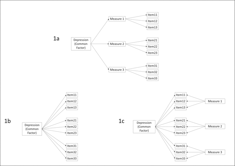
Causal models of construct equivalence. These include: (1a) equivalence at the measure level; (1b) equivalence at the item level; (1c) equivalence at the item level after accounting for measure-specific effects (bifactor model).

The presence of method effects violates another key assumption of all effect indicator models: that of conditional independence (Sobel, 1997). When conditional independence holds, any associations among indicators are entirely accounted for by the construct (or by additional constructs specified in the model), and any residual indicator variance or measurement error remaining after construct variance has been accounted for will be independent across all indicators, reflecting causes unique to each indicator. If this assumption is violated, indicators are systematically contaminated by other constructs, and inferences based on an incorrectly specified measurement model could be biased. Bifactor models can be used to test whether method effects lead to such contamination.

A third major assumption of construct equivalence is that of causal invariance: the causal model underlying measurement is assumed to be invariant across a defined range of application. When applied to data synthesis, we assume that the effect of the construct on its indicators will be invariant for the set of studies included in the analysis. In addition, causal invariance would imply that the effect of the construct on its indicators will not vary across sample characteristics such as age or sex; nor will it vary across different intervention conditions, or across studies conducted in different environmental contexts, or across trials. Each indicator is assumed to be influenced by the construct in the same way regardless of respondent, condition, context, or trial. When these assumptions are violated, data are said to exhibit differential item functioning (DIF), meaning that the causal association of the construct with its indicators varies across one or more of these domains (Millsap & Everson, 1993).

Equivalent indexing, a final assumption of construct equivalence, involves the strength and nature of causal impact of the construct on its indicators. Some indicators of a construct may be influenced more strongly than others, and the effects may differ in functional form (e.g. linear, curvilinear, or discontinuous impact of construct on indicator). This must be considered when determining how much and in what way an indicator value indexes the value of the construct, and how a set of indicators are combined in that indexing. Full construct equivalence assumes that this indexing process leads to equivalent values on the construct across different measures.

Statistical Methods for Testing Assumptions

There is a substantial research literature on linking and equating measures of the same construct, much of it in the educational field (Dorans, Pommerich, & Holland, 2007). Most of this work focuses on total scores and uses measurement studies specifically designed for this purpose. Here we focus on methods that can be applied post hoc to an existing set of studies using different measures of ostensibly identical constructs. Unlike equating studies, these studies are not designed specifically for equating measures; rather they are assembled to test the same hypotheses about the same construct and provide a corpus of research for data synthesis using meta-analytic or IDA methods.

Approaches using item-level data, involving application of item response theory (IRT) methods (Yen & Patrick, 2006), have also been employed for measure equating, and here we extend this approach to include multiple measures across multiple studies. These have several advantages. They can handle different ordinal scales with different numbers of categories. They use all available information on item-level correlations or associations between measures, even when this is based on smaller subsets of studies. They allow for estimation of a single latent score on the construct for each participant, based on all information available. The latent score is on a common metric, regardless of which specific items contribute to its estimation for a specific participant. They do not require that the various measures have similar reliabilities or similar difficulty levels, as is the case with many methods based on total scores. Most important for this paper, IRT modeling allows for direct tests of measurement assumptions involving common cause, conditional independence, and causal invariance. And if violations are found, these models can be used to explore whether measures can be revised to estimate latent scores that do not violate these assumptions.

Common Cause

In a synthesis dataset with item-level data for all participants, we can test the common cause assumption by specifying a basic IRT model where all indicators load on a common construct (consistent with the causal model in Figure 1b), and determining which loadings are significant and in the same direction. This statistical model includes all indicators from all measures. For polytomous indicators, Samejima’s graded response model (Samejima, 1969), presented below, is the most commonly used IRT model. In this model, let y_ij denote the categorical response of the ith subject on the jth item (i=1, …, n; j=1,…, J), and the response categories are k = 0,…, m − 1. Note that J reflects the total number of items across all measures, not the number within each measure. The probability of person i endorsing the jth item is given by ${\pi }_{ij}=P\left(y_{ij}=k|{\theta }_{ci}\right)$ and is expressed via the logistic cumulative distribution function as

$$P\left(y_{ij}=k|{\theta }_{ci}\right)==\{\begin{array}{cc}1-\mathrm{\Psi }\left({\alpha }_j{\theta }_{ci}+{\beta }_{0jk}\right)& \text{ if k}=0\\ \mathrm{\Psi }\left({\alpha }_j\theta c_i+{\beta }_{0jk}\right)-\mathrm{\Psi }\left({\alpha }_j{\theta }_{ci}+{\beta }_{0j,k+1}\right)& \text{ if }0<\text{k}<\text{m}-1\\ \mathrm{\Psi }\left({\alpha }_j{\theta }_{ci}+{\beta }_{0j,k+1}\right)& \text{ if k}=\text{m}-1\end{array}$$ (1)

Here θ_ci is the common trait for i-th subject; α_j is the loading (slope) of the j-th item on that common trait, also called the item discrimination parameter, reflecting the strength of the common trait’s impact on each of the j items. β_0j is the intercept parameter for the jth item; this indexes item severity. The intercept is inversely related to the threshold (Cai, Ji Seung, & Hansen, 2011), another location parameter commonly used in IRT models. For ordered polytomous indicators, the threshold is the expected value of the latent variable $\mathrm{\theta }$ at which an individual transitions from one scale level to the next. Items with lower intercepts (or higher thresholds) imply that a respondent would likely be higher on the common trait before endorsing the item. The corresponding link ψ is logistic, i.e., ${\mathrm{\psi }}^{-1}(\text{p})=logit\left(P\left(y_{ij}=k|\theta \right)\right)={\alpha }_j{\theta }_{ci}+{\beta }_{0jk}$. The index i runs over all subjects i = 1, …, n, and the index j refers to items 1 to J. A normal cumulative distribution function (CDF), or probit model, is often used as an alternative to the logistic CDF in equation (1).

This model provides a means of testing the common cause assumption. If we fit this model to a dataset that combines items from all measures, the common cause assumption will be upheld if all α_j parameters are significant and have the same sign. If some of the α_j parameters are small and do not reach significance or are negative (when item scaling assumes a positive association), the associated indicators can be dropped from the model, resulting in a measurement model that agrees with this assumption. This can occur if a measure that purports to index the general construct includes some indicators that are not found in other measures. For example, all questionnaire measures of youth depression include items about sad mood, but items concerning social relationships are found in only a few depression measures, and may not be associated strongly enough to meet the assumption of common cause for the entire set of indicators.

Conditional Independence

Tests of conditional independence require that we identify plausible confounding factors that could contribute to correlations among indicators above any associations due to the common construct. Violations of conditional independence can take many different forms, including correlations among one or more pairs of item residuals. When multiple measures are included, violations due to shared method factors should always be considered plausible, given the ubiquity of method effects in psychological measurement. For individual-level saturated datasets method effects can be tested with multidimensional methods such as the bifactor statistical model that tests assumptions of a causal model such as that illustrated in Figure 1c.

The bifactor model extends the model in equation 1 by including both a common latent factor and two or more secondary factors. For the bifactor model, Given S secondary latent factors, let θ_si index the s-th secondary latent factor θ_si (s=1, …, S), and θ_ci the common latent factor. The probability of endorsing the j-th item is given by $P\left(y_{ij}=k|{\theta }_{ci},{\theta }_{si}\right)$

$$\begin{gathered} P\left(y_{ij}=k|{\theta }_{ci},{\theta }_{si}\right)= \\ \{\begin{array}{cc}1-\mathrm{\Psi }\left({\alpha }_{cj}{\theta }_{ci}+{\alpha }_{sj}{\theta }_{si}+{\beta }_{0jk}\right)& \text{ if k}=0\\ \mathrm{\Psi }\left({\alpha }_{cj}{\theta }_{ci}+{\alpha }_{sj}{\theta }_{si}+{\beta }_{0jk}\right)-\mathrm{\Psi }\left({\alpha }_{cj}{\theta }_{ci}+{\alpha }_{sj}{\theta }_{si}+{\beta }_{0jk+1}\right)& \text{ if }0<\text{k}<\text{m}-1\\ \mathrm{\Psi }\left({\alpha }_{cj}{\theta }_{ci}+{\alpha }_{sj}{\theta }_{si}+{\beta }_{0jk+1}\right)& \text{ if k}=\text{m}-1\end{array} \end{gathered}$$ (2)

The probability of endorsing the jth item is related to a linear function of the latent variables through a link function g(.),

$$g\left(P\left(y_{ij}=k|{\theta }_{ci},{\theta }_{si}\right)\right)={\alpha }_{cj}{\theta }_{ci}+{\alpha }_{sj}{\theta }_{si}+{\beta }_{0jk}$$ (3)

where g(.) is the logit (or probit) link for a polytomous response; α_cj and α_jk are the loadings (slopes) of the jth item on the common (θ_ci) and specific latent variables (θ_si), respectively; and β_0jk is the intercept parameter for the jth item and kth response category (k = 0, …, K). Note that the latent variables are assumed to be uncorrelated (DeMars, 2006) and to be normally distributed.

If the specific latent variables reflect specific measures, significant loadings α_sj provide evidence that the conditional independence assumption is not met, because correlations among indicators within a measure are more strongly associated than would be predicted by the simple common factor model. If such effects are relatively weak, violation of this assumption may not have substantive implications for construct equivalence. If the effects are robust, the bifactor model may be used to adjust for them. Under the assumption that lack of conditional independence is entirely due to method factors, including those factors in the model will allow for the estimation of the common factor independent of these effects. In the most extreme case, method factors may account for most of the item variance (Gibbons and Hedeker, 1992). In this case we would need to consider the possibility that the constructs as measured by different methods are not substantively equivalent. In the current study we consider source of rating (youth, parent, clinician) as potential method factors, and test whether they account for variance in items over and above that accounted for by a general depression factor. We also test models that include only youth report, and consider specific questionnaire sources as potential method factors.

Estimation of bifactor IRT models with binary or ordinal indicators requires numerical integration estimation procedures. Under the standard assumption that all factors are independent of each other, this model can be specified as a two-level model, requiring only two dimensions of integration, greatly reducing processing time (Gibbons & Hedecker, 1992). Bifactor models are ideal for data synthesis applications, given that combining data from multiple studies with different measures can increase the likelihood of significant method effects. If significant method factors are found, the bifactor IRT can be used to produce scores that have been adjusted for this source of bias.

Invariance

As with conditional independence, we need to identify plausible conditions that could lead to variation in our measurement model across individual or trial level covariates available in the particular set of studies in our dataset. Is there empirical or theoretical rationale for suspecting that measurement could be influenced by population characteristics such as age or sex? Could the studies in our synthesis set have been conducted across a range of contexts that might alter responses to our measures (such as school-based versus clinic-based venues)? Could our studies vary in terms of how the same measures were administered in different ways (in person, by phone, over the internet), and is there good reason to suspect that this might have influenced measurement response? These can include both individual-level characteristics (such as age or sex) as well as study-level characteristics (mode of administration). Given that the number of possible moderators could be quite large, we emphasize the importance of considering only those plausible conditions supported by theory or other empirical findings. In this study we focus on sex and age, given evidence that depressive symptoms become more common for girls as they move through adolescence.

Invariance assumptions can be violated in several ways. Steencamp and Baumgartner (1998) reviewed the expanding literature on measurement invariance, identifying several types of violation and describing methods for testing invariance assumptions through confirmatory factor analysis. These include include tests of configural, metric, and scalar invariance. In the IRT tradition, these are considered different aspects of differential item functioning, or DIF. Configural invariance (Horn & McArdle, 1992) is the assumption that the items of a measure will exhibit the same pattern of salient and nonsalient factor loadings across the population or contextual characteristic of interest. From the perspective of construct equivalence, this would reflect invariance of common cause across population or context. Metric invariance (analogous to nonuniform DIF in the IRT literature) is the assumption that the magnitude of an item’s loading on a factor will be equivalent across population or context. In terms of construct equivalence, this reflects the assumption that the construct of interest will have the same strength and form of impact on an indicator regardless of population or context. Scalar invariance (analogous to uniform DIF in the IRT context) is the assumption that an item’s intercept (or thresholds in the case of categorical indicators) will be equivalent across population or context. For construct equivalence, scalar invariance involves mapping of construct range onto item range. Items often vary in severity, such that item variation is shaped by variation in the underlying construct only across a particular range of that construct. Scalar invariance is present when an item’s mapping is the same across population or context.

If violations of conditional independence are present and we need to incorporate other factors (such as source of rating) to adjust for method variance, this raises the question of whether invariance is required for both the construct of interest (as indexed by the common factor) and any method effects (as indexed by specific factors). To our knowledge this topic has received little attention. One possibility is to require invariance for parameters of the construct of interest, but not for parameters involving method effects. This allows the structure of method factors to vary across population or context, as long as the structure of the common factor remains invariant. This would allow for nuisance factors that operate in different ways for different subpopulations, while still maintaining the requirement that items index the construct of interest in the same way across the entire population. We employ this strategy here.

Tests of invariance in the IRT framework can be conducted with structural equation models through multigroup modeling, allowing for comparison of item parameters across groups defined by population or contextual characteristics. Taking sex as an example, for the single common factor model, the probability of endorsing the jth item is now given by $g\left(P\left(y_{ij}=k|{\theta }_{ci}\right)\right)$, where

$$g\left(P\left(y_{ij}=k|{\theta }_{ci}\right)\right)={\beta }_{0jk}+{\beta }_{1j}{G}_i+{\beta }_{2j}\left({\theta }_{ci}*G_i\right)+{\alpha }_{cj}{\theta }_{ci}$$ (4)

with G_i = 1 for female (focal group) and G_i =0 for male (reference group). The intercept parameters now involve two components, β_0jk and β_1jG_i. The new parameter β_1j indexes intercept differences between females and males for each item, reflecting violations involving uniform DIF. Likewise the slope parameter also includes two components, α_cj and β_2j. The new parameter β_2j indexes differences in item loading due to sex, which would demonstrate violations involving nonuniform DIF. Significant nonuniform DIF indicates that responses to an item index higher (more severe) levels of the latent construct for one group; significant uniform DIF reflects differential sensitivity of the item to differences in the latent construct.

This model can also be specified as a multigroup model. Taking sex as an example, the probability of a female endorsing the jth item is now given by $g\left(P\left(y_{ij}=k|{\theta }_{ci},G=F\right)\right)$, and for a male by $g\left(P\left(y_{ij}=k|{\theta }_{ci},G=M\right)\right)$, where

$$\begin{gathered} g\left(P\left(y_{ij}=k|{\theta }_{ci},G=F\right)\right)={\beta }_{F0jk}+{\alpha }_{Fcj}{\theta }_{ci} \\ g\left(P\left(y_{ij}=k|{\theta }_{ci},G=M\right)\right)={\beta }_{M0jk}+{\alpha }_{Mcj}{\theta }_{ci} \end{gathered}$$ (5)

with separate item parameters for intercepts and slopes for males and females. Tests of uniform and non-uniform DIF involve testing whether equality constraints $\left({\beta }_{F0jk}={\beta }_{M0jk}\right)$ and $({\alpha }_{Fcj}={\alpha }_{Mcj})$ worsen model fit. Such tests may also be conducted with thresholds rather than intercepts.

Differential item functioning can also operate in bifactor structures, although this issue has received very limited attention as yet (Jeon, Rijmen, & Rabe-Hesketh, 2013). Based on the same notations considered above, the full bifactor multigroup model is written as

$$\begin{gathered} g\left(P\left(y_{ij}=k|{\theta }_{ci},{\theta }_{si},G=F\right)\right)={\beta }_{F0jk}+{\alpha }_{Fcj}{\theta }_{ci}+{\alpha }_{Fsj}{\theta }_{si} \\ g\left(P\left(y_{ij}=k|{\theta }_{ci},{\theta }_{si},G=M\right)\right)={\beta }_{M0jk}+{\alpha }_{Mcj}{\theta }_{ci}+{\alpha }_{Msj}{\theta }_{si} \end{gathered}$$ (6)

If we consider the specific factors θ_si to be nuisance factors, then we can assume that group differences in those factors do not violate the invariance assumption and can focus on testing invariance in the common factor. In this case α_Fsj and α_Msj would be allowed to vary as tests for invariance in item intercepts and slopes using equality constraints described earlier. These models test invariance across single categorical variables such as sex. Curran et al. (2014) have recently extended moderated nonlinear factor models to synthesis datasets, allowing for evaluation of more complex patterns of non-invariance involving multiple continuous moderators. Computational complexity of this approach increases substantially as the number of items increases and may not be feasible at present when an IDA dataset includes several measures and many items.

For synthesis analysis, interpretation is easier when we also assume that intercepts and slopes do not vary across studies. This can in principle be evaluated through multigroup models. However, the number of free parameters in these models increases multiplicatively with the number of studies, and estimation can be intractable with current frequentist statistical methods. For example, the dataset we employed here includes 16 trials, and a model testing cross-study invariance for a single latent variable would include 6260 free parameters. In the future, Bayesian methods may hold promise for estimating complex models of this sort having many parameters (Gelman et al., 2013).

Equivalent Scaling

Different measures of the same construct usually provide different ways of quantifying that construct, based on the number of indicators and how those indicators are themselves scaled. We need to have a method for combining indicators within a measure, and of aligning quantification across measures. This is of central importance when we are interested in synthesizing data concerning mean differences, as in the prevention trials data we use here.

With individual-level data we can carry these out within the IRT model itself. The model estimates relative contributions of each indicator to the construct (based on the strength of the construct’s effect on the indicator), and also estimates intercepts for each step in the ordered set of categories that quantify each indicator. These parameters can then be used to estimate a factor score for each participant based on all available items, i.e. with an empirical Bayes estimate along with its standard error. The resulting factor scores are on a common metric, even if the items have different numbers of categories, and different participants have data on only a subset of items.

In summary, several statistical methods are available for testing the assumptions underlying construct equivalence, and for adjusting measures to reduce or eliminate violations that are detect. Having individual-level and item-level data greatly enhances the opportunities for testing these assumptions prior to conducting meta-analyses of studies employing multiple measures of the same construct.

Testing Construct Equivalence in Measures of Youth Depression

We applied this framework to data that included several different measures of youth depression. Data used in these analyses came from the Collaborative Data Synthesis (CDS) Project, involving 4146 youth ages 10 to 18 who participated in 16 randomized control trials of preventive interventions designed to reduce risk of depression or problem behavior (Brincks et al., 2017; Brown et al., 2017). These trials used seven different measures of depression, a total of 123 items, but each trial used one, two or at most three of those measures. Trials varied in sample size from 49 to 667. We combined pretest data from these trials into a single dataset. There is substantial missing data for each trial, in that trials only used a subset of possible measures. As this study involved secondary analysis of de-identified data, the XXX IRB determined that the study was exempt from review.

The combined sample was 50.3% female. A few trials included younger children or young adults; we used data from those who ranged in age from 10 to 18. Mean age was 12.9, weighted towards early to middle adolescence (44% in ages 10 to 12; 48% in ages 13 to 15; 9% in ages 16 to 18.) Four of the trials sampled only Hispanic youth, and several others had smaller Hispanic subsamples, such that the entire sample was around 40% Hispanic. Racial breakdown of non-Hispanic youth was 13% Black, 79% White, 2% Asian, and 6% other. Sample characteristics for each trial are reported in detail in on-line Supplementary Materials Table S1.

The seven measures used in these studies included four youth self-report questionnaires: the 27-item Child Depression Inventory (CDI: Kovacs, 1992), 20 items reflecting depressive symptoms from the Youth Self Report Form (YSR: Achenbach, 1991a), the 20-item Center for Epidemiologic Studies Depression Scale (CESD: Radloff, 1977), and a 14-item scale developed for the Project Alliance trials (PAL: Dishion et al., 2002). They also included two parent report questionnaires: 20 items reflecting depressive symptoms from the Child Behavior Checklist (CBC: Achenbach, 1991b) and 5 items reflecting depressive symptoms from the Behavior Problem Checklist (BPC: Quay & Peterson, 1993). One clinician rating form, the 17-item Child Depression Rating Scale (CDRS: Poznanski & Mokros, 1996), was also included. Given that the CBCL, YSR, and BPC have standard subscales that combine depression and anxiety, we selected only those depression items that had content overlap with the other measures. All items used in these analyses are listed in Table S2 in on-line supplementary materials.

Testing Common Cause Assumptions

Modeling item-level synthesis data presents several challenges. The total number of items can be much larger than is commonly found in studies of measurement invariance for a single measure. In our example, the CDS dataset includes a total of 123 items from 7 measures at baseline, which is the single time point we used in this study. Simpler models that assume interval scaling may be possible when all items have five or more scale points but are not appropriate when items have fewer scale points (Bandalos & Enders, 1996). Four measures (BPC, CBC, YSR, CDI) used 3 scale points, two measures (CDRS, CESD) used 4, and one measure (PAL) employed 5. Frequency of usage was strong across the full range of scale scores, arguing against collapsing across scale points in all but a few cases. Nine items had very low frequencies in their highest categories, so we merged those responses with the next highest category. In this case direct modeling of categorical data using an IRT approach is required. We first estimated a single common factor IRT model for our synthesis dataset using MPLUS version 8 (Muthén & Muthén, 1998–2010).

IRT models can be estimated using weighted least squares mean and variance (WLSMV) estimators, or maximum likelihood (ML) estimators using numerical integration. In this case WLSMV proved impossible because of the pattern of missing data. That approach requires that all pairwise item correlations be directly estimable. This will be true for a synthesis dataset only when every pair of measures is utilized together in at least one study contributing to the dataset. This is not the case with the CDS dataset, which includes only 7 of the 21 possible pairwise combinations. We therefore used ML with numerical integration, along with the full information maximum likelihood option, which utilizes all data in estimation, regardless of the pattern of missingness. MPLUS allows for including indicators with different numbers of response categories, so all 123 items were allowed to load on the common factor, using a graded response model for ordered categorical data. See Program Appendix 1 in the on-line supplementary materials for the MPLUS code.

This estimation method assumes that observations are all independent; if this assumption is violated then estimation of standard errors may be biased. Study-level effects could result in non-independent data. When possible, we used the COMPLEX option in MPLUS to adjust standard errors for any clustering by study using a sandwich-type estimator of the variance.

The estimation procedure reached convergence; parameter loadings on the single common factor were significant at the p < .001 level for 107 of the 123 items (see Table S2 in on-line supplementary materials for a complete list of all parameters). These findings provide some support for the common cause assumption for most of the items. However, all but one of the 16 non-significant items were from the clinician-reported CDRS and the parent-reported BPRC, suggesting that these two measures were not strongly shaped by this single common factor.

Testing Conditional Independence Assumptions

Most investigators treat youth depression as a unitary construct that can be assessed through different methods. The synthesis dataset includes seven different measures: four use youth report, two use parent report, and one involves clinician report. Given evidence that measures may not always correlate highly across different reporters (Achenbach, McConaughy, & Howell, 1987), we decided to test whether reporter factors might account for variation in items independent of that accounted for by the common factor, violating the conditional independence assumption. We therefore specified and estimated a bifactor IRT model with a common factor and three secondary reporter factors. We used a graded response model for ordered categorical data, similar to that specified for the single common factor model described earlier, adding three secondary latent factors, each loading on items from a separate reporter (youth, parent, or clinician). Correlations among the common factor and the three secondary factors were all forced to zero, as required by the bifactor model. See Program Appendix 2 in the on-line supplementary materials for the MPLUS code.

Results indicated that items were strongly influenced by reporter factors. The BIC for this model was much smaller than that for the single factor model (bifactor BIC = 181,682, single factor BIC = 175,734), indicating the bifactor model fit far better. Loadings from this model are reported in supplementary Table S2. All but one of the loadings on the youth, parent, and clinician reporter factors were positive and significant at p < .001. Loadings on the common factor are changed substantially; 28 items now have negative loadings (including all items from the youth-reported PAL and parent-reported BPC), even though item content is scored in the same direction as other items. Of the remaining items 57 do not reach significant levels of p < .001.

Assessing bias due to violations of conditional independence.

Violations of conditional independence detected through bifactor modeling may not be severe enough to bias estimates even when simpler single factor models ignoring these violations are used to test associations with other variables such as intervention status. Reise, Scheines, Widaman, & Haviland (2013) found that such bias will depend on both the estimated common variance (ECV) and the percentage of uncontaminated correlations (PUC) for a bifactor model. ECV is defined as the proportion of common variance attributable to the common factor (as compared to the total variance attributable to all factors); PUC refers to the proportion of observed correlations among all observed indicators that involve indicators from different secondary factors. The ECV for the bifactor model was very modest, with the common factor in that model accounting for 11.7% of the common variance, and reporter factors accounting for the remainder. This is likely an over-estimate, as 23% of the loadings on the common factor used to estimate the ECV were negative (loadings are squared and summed to calculated ECV), accounting for almost 30% of that figure.

Reise et al. also demonstrated that lower ECVs may not lead to significant bias if the PUC for the model is large and provided tables from simulated data suggesting relative cutoffs indicating significant bias when PUC was below 69% and the ECV was below 58%. The PUC for our bifactor model was 58%, and in conjunction with the very modest ECV suggested that a single common factor model for youth depression based on indicators from all three reporters would be seriously biased.

Standard meta-analyses calculate effect sizes based on intervention and control group means standardized on study sample standard deviations. As another check on the likely impact of using scores from multiple reporters in a basic meta-analysis, we calculated and standardized intervention group and control group means based on summed scores of all depression measures. We also calculated similar means based on estimated common factor scores from our bifactor model for each trial. These two sets of trial-level means correlated −0.01, indicating essentially no commonality between means based on the common factor in the bifactor model and means based on simple standardized summary scores (see Figure S1a in the supplementary materials for a scatterplot of this association).

Exploring separate single factor models.

These findings strongly suggested that items from different reporters were only weakly indexing the same construct, and that the clinician ratings were essentially uncorrelated with youth ratings. We therefore decided to explore a two-factor model which included separate latent variables for youth and parent report, allowing these factors to correlate. Because the three studies using clinician ratings also included parent or youth reports, we could drop clinician ratings without losing studies from the sample. Item loadings were all strong and statistically significant for the two latent factors, with one exception (CES-D item 7, worded as “I felt that everything I did was an effort”, had a weak and non-significant loading on the youth reporter factor). The two factors were modestly correlated (r = .285, SE = .029, p < .001).

We also estimated a bifactor model with two secondary factors that excluded clinician ratings and included only parent (N=25) and youth (N = 81) items. Although the BIC suggested a better model fit for the bifactor model compared to the two correlated factors model (bifactor model BIC = 158,161; two correlated factor model BIC = 158,966), the common factor in the bifactor model showed problems similar to those in the earlier models: only 12 of 106 items had significant positive loadings, and 10 items had reversed loadings with a significant negative parameter, suggesting that most of the item variance was not due to the common factor. In comparison, all items but one loaded significantly on their respective factors in the two correlated factors model.

In summary, items in this dataset did not meet assumptions for construct equivalence. There were substantial violations of conditional independence, and when within-reporter dependence was modeled, evidence for a single construct was weak. These findings suggest that data synthesis with these measures should be conducted separately for youth and parent reports, although this introduces ambiguity concerning the nature of the separate constructs these measures index. We discuss this issue in greater detail later.

Testing Assumptions for Single Reporter Measures

Given these findings, we decided to test whether measures based on only one reporter were more likely to meet assumptions for construct equivalence. We focused on youth report measures, given that less than half of the participants had parent reports (N = 1900). We followed a similar strategy for evaluating construct equivalence, estimating a single factor model with all 81 youth report items to test the common cause assumption. All but one item loaded significantly on this single factor (see Table S3 in supplementary materials), providing support for this assumption. We then estimated a bifactor model that included four secondary factors, modeling variance unique to each of the four youth measures, to test for violations of conditional independence due to measure-specific variance. Model comparison tests (Table 1) indicated that the bifactor model fit significantly better than the single factor model. All but eight items continued to load on the common factor in the bifactor model, supporting the common cause assumption. However, several items (27 of 81) also loaded significantly on specific measure factors, particularly those for YSR and PAL2D items, indicating that conditional independence was violated (see Table S3 in supplementary materials).

Table 1.

Tests of sex invariance for youth report measures through comparison of relative fit of configural, metric, and scalar models.

Model	LL	AIC	BIC	Parm	Difference in −2LL	Difference in parm	p< for test of difference
Comparing Single and Bifactor Models1
Single Factor	−62835.4	126248.7	128054.6	289
Bifactor	−62024.1	124788.1	127100.1	370	1166.7	81	.001
Tests of Bifactor Model Invariance Across Sex2
Configural Invariance3	−64095.8	129669.6	134287.3	739
Metric Invariance4	−64154.1	129624.9	133742.7	659	116.6	80	.005
Scalar Invariance5	−64525.9	129957.7	132788.3	453	743.5	206	.001
Tests of Bifactor Model Invariance Across Age2
Configural Invariance3	−56149.9	113441.8	116945.8	571
Metric Invariance4	−56201.8	113413.6	116512.5	505	103.7	66	.005
Scalar Invariance5	−56373.8	113457.5	115636.0	355	343.9	150	.001

¹Sartorra-Bentler robust chi-square for MLR estimation.

²Standard chi-square for ML estimation.

³Loadings and thresholds of main factor free across sex.

⁴Loadings of main factor fixed to equal, thresholds free across sex.

⁵Loadings and thresholds of main factor fixed to equal across sex.

We calculated ECV and PUC for this bifactor model to assess whether these violations would bias estimates based on a single common factor model. The common factor in the bifactor model accounted for 59% of the estimated common variance, and the PUC for this model included 75% uncontaminated correlations. Simulations reported by Reise et al. indicated that for substantive bias the ECV would need to be below 50% for a model having a PUC of 75%, suggesting that these violations of conditional independence would not lead to problematic levels of bias. We also calculated experimental and control group means on standardized summary scores and factor scores based on the bifactor model. These were strongly correlated (r = .56), indicating significant though not perfect commonality (See Figure S1b in supplementary materials for a scatterplot of this association).

We next conducted tests of invariance across sex and age for the common factor in the bifactor model. We first estimated separate bifactor models for males and females, and then compared loadings and thresholds for each item. We selected an index item that loaded strongly on the common factor, loaded minimally and non-significantly on its respective source factor, and had loadings and thresholds that differed the least across sex. The loadings for this item (CDI item 13: “I cannot make up my mind about things”) were forced to 1 and thresholds were forced to the values estimated in the basic bifactor model. We then freed means and variances across sex for the common factor, forcing them to 0 and 1 respectively for the source factors. We also allowed all loadings and thresholds to be free and differ across sex for all source factors.

We used these specifications for all three invariance models (See Program Appendices 3, 4, and 5 for MPLUS code). The configural model allowed all other common factor loadings and thresholds to be free and differ across sex; the metric model forced all other common factor loadings to be equal across sexes, with thresholds remaining free; and the scalar model forced both common factor loadings and thresholds to be equal across sexes. We reduced the number of integration points per dimension to 8, given the computing demands of a bifactor model with one common and four secondary factors. Table 1 summarizes model fit statistics for these models.

Tests of sex invariance with the bifactor model indicated that item loadings for the common factor showed significant violations of both metric and scalar invariance (see Table 1). Violations of invariance assumptions can in principle bias scores and score equating (Kabasakal & Kelecioglu, 2015), but statistically significant bias may not in fact be strong enough to make a practical difference (Wanders et al., 2015). To assess the seriousness of these violations, we used MPLUS to calculate empirical Bayes estimates of the common factor scores for the basic single factor model and the configural model, regressing the former on the latter separately for females and males. Figure 2a illustrates the resulting predicted regression lines. In both cases the single factor score under-estimates the configural factor score for higher levels of depression, and over-estimates the adjusted score at lower levels. Violation of assumptions appear to have a much stronger effect on scores for males (b = 0.504, simple r = .776) than for females (b = 0.811, simple r = .939). For example, for those scoring at the mean on the basic single common factor males are 0.19 SD below females on the corrected score, and for those scoring two standard deviations above the mean, males are 1.03 SD below females on the corrected score.

Figure 2.

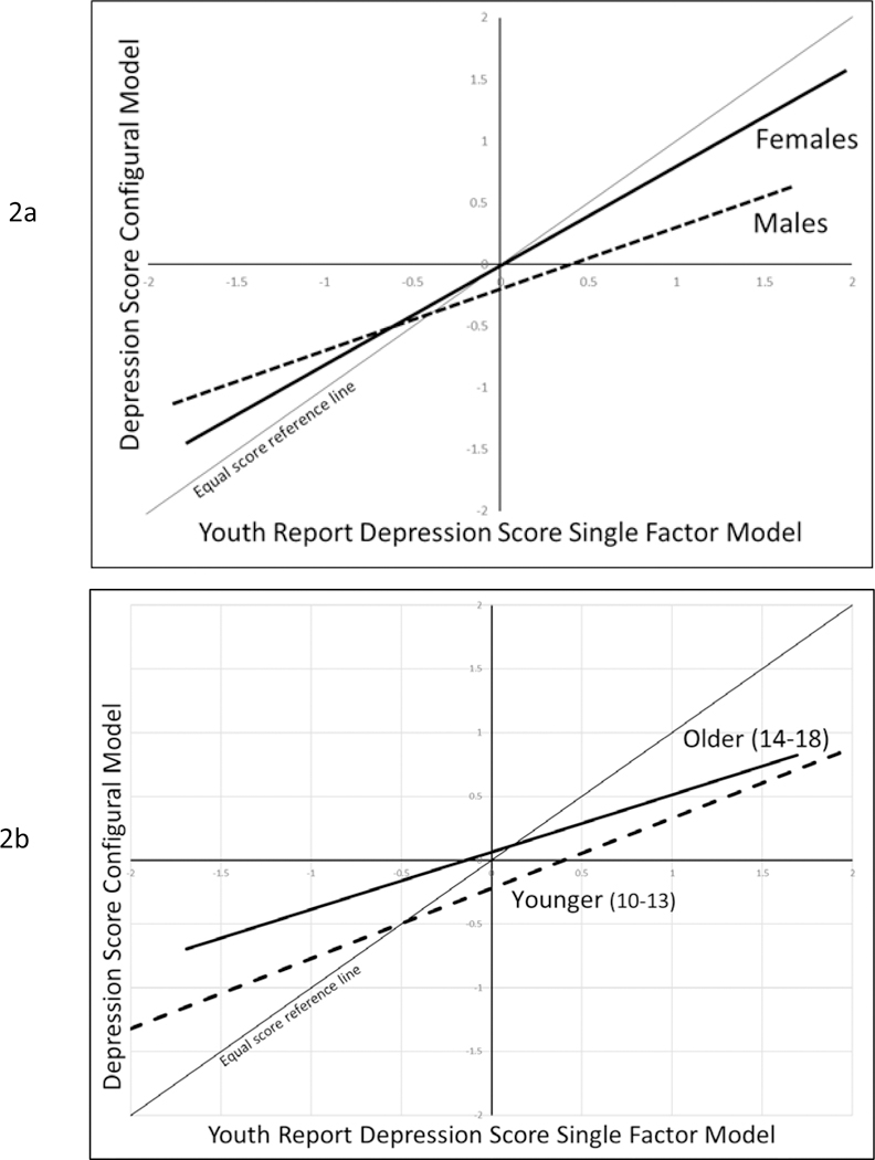
Predicted regression lines illustrating associations between youth report common factor scores from the single common factor model and the configural model (based on bifactor model with four specific measure factors). Lines cover the range of −/+ 2 SD on single factor model scores.

We attempted to repeat these analyses to test invariance across age, dividing the sample into younger (10–13) and older (14–18) age ranges. Unfortunately, one of the measures (the PAL2D) had only been used in trials that included youth between 10 and 13. Although not strictly comparable, we decided to conduct exploratory tests of age invariance on a subsample that included the remaining measures (N = 3417). We therefore tested age invariance for the common factor in a bifactor model that included only 3 of the youth report measures. Invariance tests for the common factor found that both metric and scalar invariance were again violated (see Table 1). Graphs of empirical Bayes estimates of factor scores (Figure 2b) suggest that the single factor model over-estimates depression scores at the lower end of the scale, and under-estimates them at the higher end, for both younger and older youth. Violation of assumptions appears to be somewhat stronger for youth aged 10–13 (b = 0.449, simple r = .755) compared to youth aged 14–18 (b = 0.551, simple r = .860). For example, younger youth scoring at the mean on single factor scores are a quarter of a standard deviation lower on the configural score than older youth.

Conclusions and Future Directions

We began by reviewing the assumptions underlying construct equivalence, a necessary condition for synthesizing data across multiple studies, noting the limited capacity of meta-analysis to test these assumptions. We then described an analytic strategy for testing these assumptions using individual participant data combined from multiple studies, extending concepts from measurement theory to this more complex case.

Applying this strategy to item-level data from measures of youth depression, we found evidence for violation of the assumptions of common cause and conditional independence. Findings indicated that reporter effects were strong, clinician ratings were essentially independent of any common factor, and parent and youth ratings formed separate factors that were only weakly correlated with each other. These violations would lead to substantial bias when used in either IDA or standard meta-analysis. Separate analyses of the youth items found stronger evidence for the utility of a single common factor model, although we also found violations of the invariance assumption across sex and age.

What are the implications of these findings for data synthesis? These measures of depressive symptoms were used to test the effects of prevention programs using randomized controlled trials. Our findings suggest that using standard meta-analytic methods with these data could lead to biased results. Measures based on different reporters do not appear to be indexing the same construct or are doing so only weakly. There is stronger evidence that different measures from the same reporter are indexing the same construct, at least for youth reports. However, youth report data also violated assumptions for conditional independence (due to within-measure effects) and invariance across sex and age. We were able to estimate IRT models that adjusted a general depression factor to control for these effects and would recommend exploring such adjustments in future synthesis analyses combining data from these trials to study intervention impact across trials.

Our findings also have general implications for efforts to synthesize data across multiple studies. It demonstrates that psychometric modeling is possible with sparse synthesis data and may be able to yield results not possible on smaller and more restricted datasets from individual studies. Range restrictions are less likely to be a problem because multiple studies using the same measure are likely to increase the range of scores for the synthesis sample as a whole. Synthesis datasets also provide substantial increase in the number of participants, and larger datasets help both to stabilize estimation of complex models and allow for detection of more subtle violations of measurement assumptions.

These findings are also relevant for assessing the psychometric validity of measures of youth depression. Use of multiple reporters presupposes construct equivalence across those various reports. Different reporters likely use different sources of information (internal experiences for youth, observations of youth behavior and report by parents or clinicians), but these reports must correlate for them to demonstrate construct equivalence. When measures of youth depression from multiple reporters are included, our findings indicate that reporter effects may present a strong challenge to the assumption of conditional independence, and reduce confidence in construct equivalence. Bifactor approaches that directly model reporter effects find that much of the variation in depression items is specific to reporter, rather than reflecting a common underlying construct.

Findings of low cross-reporter consistency in other individual studies fit this pattern (Achenbach et al., 1987), although such findings are not always consistent across studies. For example, in the dataset used here, three studies employed both the clinician-rated CDRS and the youth-rated CES-D. Combining data across these three trials, these two measures are correlated r = .28 at baseline. In comparison, a recent study of children and youth with asthma (Lim, Wood, Miller & Simmens, 2011) found these measures correlated r = .62.

Achenbach et al. (1987) initiated a broader discussion on multiple informant data that has highlighted two major themes: context specificity and differential bias. Achenbach et al. suggested that child behavior problems may be context-specific, and so the construct itself should take into account variation across context. Most of the subsequent work on this thesis has focused on externalizing behavior or social anxiety (De Los Reyes et al., 2015). We have seen little on considering context-specificity of youth depressive symptoms, and in fact all the trials included in our analyses conceptualized depression as general rather than context-specific.

De Los Reyes et al. also raised the issue of differential bias, suggesting that different reporters can be biased by different cognitive processes including attributions about the cause of behavior and differential attention to specific subsets of symptoms. These effects would contribute to measurement error and are very consonant with our bifactor model approach. The IRT models we employed are more sensitive to such effects in two ways: they build on cross-reporter correlations which should be higher if both reporters are picking up on the same underlying construct, and they allow for different items to load more strongly on the common factor for different reporters, reducing the impact of attention bias should it be present.

Several studies have also tested measure invariance for single measures of youth depression (e.g. Pei-Chen & Tsai-Wei, 2014), but we have been able to locate only one prior study including items from multiple reporters in tests of construct equivalence. Bauer et al. (2013) presented analyses of data incorporating both mother and father report of child negative affect into a trifactor model that includes a common factor, reporter factors for each parent, and item-specific factors for each item (given that both parents reported on identical sets of items). Consistent with the current study, they found strong reporter effects in addition to a common factor. They were able to test for differential item functioning across reporters, finding evidence for scalar DIF across reporters in 4 of the 13 items studied. In the future this approach could be extended to determine whether confounding of reporter and measure could also add bias to measurement. In addition, some specific symptoms of depression may be more accurately assessed through multiple reporters than others, suggesting that these methods may prove useful in exploring which components of depression are best assessed in this way.

Findings from this study and others indicate the presence of reporter bias and sex differences that compromise the validity of current measures of youth depression. Recent advances that apply IRT modeling and computerized adaptive testing hold promise in building next-generation measures that are less sensitive to such problems (Beiser, Vu, & Gibbons, 2016).

These findings must be considered in the light of several limitations. Measures of youth depression based on this set of prevention trials may have constraints that reduce generality to other populations, particularly those involving samples with more severe depression. These trials have strong representation of Latino youth but are limited in terms of African Americans or Asians, suggesting caution in generalizing across race or other ethnicities. Individual studies have reported some evidence of differential item functioning in youth measures due to racial or ethnic variation (Crockett et al., 2005), and the current study did not test for such effects.

These methods required the use of full-information maximum likelihood estimation with a dataset having substantial missing data at the trial level, in that each study used only a subset of the measures. These analyses assumed the data were missing at random, consistent with other studies that have explored measurement models with synthesis datasets (Bauer et al., 2013). This amount of sparseness is not unusual for synthesis datasets, but it raises the question of how that sparseness might impact these analyses. Our analyses did not take into account the possibility that trial-specific decisions about measurement could violate this assumption. For example, clinical trials of interventions that target cognitive processes associated with depression may be more likely to include depression measures with more cognitive items, while antidepressant trials may be more likely to include measures that have more items related to physiological dysregulation of sleep or eating. This may not make any difference if these different items are all strong effect indicators of the same underlying construct but can bias synthesis findings if this is not the case. If this is a concern, covariates reflecting trial-level missingness of all other measures might be used to control for this form of missingness, although we were unable to fit such models with the CDS dataset, given the large number of new parameters required. Further research is necessary to determine the effects of different levels and forms of sparseness on these models, through simulations that test the impact of different patterns of missingness.

Several unanswered questions need to be addressed in future work. First and foremost, issues of construct equivalence need much greater attention in efforts at data synthesis. Meta-analysts routinely base their conclusions on assumptions that have not been carefully tested, and violations of those assumptions could have important implications for interpretation of findings from this work. This will require more efforts to share and combine individual participant data across studies (Perrino et al., 2013).

Recent advances in quantitative modeling provide an emerging platform that can support and extend this approach. Multilevel factor analytic methods for ordered categorical data are already available on general platforms such as MPLUS. Multidimensional approaches required for nonstandard bifactor modeling are also available. More flexible multilevel IRT software, recently released on stand-alone platforms such as FLEXMIRT (Cai, Ji Seung, & Hansen, 2011) are also promising, and can use Gibbons & Hedecker’s (1992) two-level dimension reduction framework for speeding up processing (Jeon et al., 2013). However, these new methods require further evaluation, given findings that some of the algorithms employed may under-estimate standard errors (Asparouhov & Muthen, 2012).

Another question involves how best to adjust for violations of invariance when faced with invariance across more than one sample characteristic (as is the case here with age and sex). It may be possible to test invariance across more than one variable at a time, and recent work on multiple group factor alignment (Asparouhov & Muthén, 2014) may prove useful. However each added variable multiplies the number of group comparisons possible, and this can lead to small cell sizes or even empty cells (as was the case in our tests of age invariance).

There are also important questions concerning the stability of construct equivalence over time. Bauer and Curran (Bauer et al, 2013; Curran et al., 2008) present methods that involve random sampling of items across time points, comparing estimated factor scores from applying the resulting model to separate cross-sectional subsets of data as a check on stability over time. McArdle et al (2009) integrate Rasch IRT modeling with growth modeling using a factor of curves approach to analyze longitudinal data combined from three studies. Multilevel IRT models hold promise for direct tests of construct equivalence over time, along with testing the necessity of such invariance for valid inference, given recent findings that longitudinal models are often robust to violations of invariance over time (Edwards & Wirth, 2012).

Analyses using individual participant data hold promise for testing whether the effects of intervention trials might be moderated by sample or context characteristics. IDA methods are much more highly powered than meta-regression methods for detecting moderation and are not subject to the ecological fallacy (Dagne, et al., 2016). The methods we employed here may be important when the goal is to test moderation, as violations of construct invariance across levels of a moderator can lead to bias in tests of moderation. In addition, we are unaware of any studies involving the harmonization of moderator variables, an issue that needs further exploration.

And finally, the assumptions of construct equivalence we tested here, while important, focus on only part of the broader issue of construct validity, which also includes theoretically motivated assumptions about more focal components of depression, such as anhedonia, or the association of youth depression with other constructs. The methods we employ here can also be used to evaluate subsets of items likely to index more specific constructs such as anhedonia, while novel methods such as meta-analytic structural equation modeling (MASEM: Hong & Cheung, 2015), particularly when conducted in the context of IDA, hold promise in testing theoretically relevant associations with other constructs. This will require that all relevant studies of youth depression measure these other constructs, so that results can be combined across studies to test these assumptions.

Public Significance Statement:

Scientists often combine data from several studies to test whether findings continue to hold. This study suggests that combining data on youth depression can be problematic when measures are completed by different reporters, such as youth or parents. It concludes that measures should be combined separately by reporter, and that statistical modeling can be used to increase the validity of combined measures.

References

- Achenbach TM (1991). Manual for the Child Behavior Checklist/4–18 and 1991 Profile. Burlington, VT: Department of Psychology. [Google Scholar]
- Achenbach TM (1991). Manual for the Youth Self Report and 1991 Profile. Burlington, VT: Department of Psychology. [Google Scholar]
- Achenbach TM, McConaughy SH, & Howell CT (1987). Child/adolescent behavioral and emotional problems: implications of cross-informant correlations for situational specificity. Psychological Bulletin, 101, 213–232. doi: 10.1037/0033-2909.101.2.213 [DOI] [PubMed] [Google Scholar]
- Asparouhov T, & Muthén BO (2012). Comparison of computational methods for high dimensional item factor analysis. MPLUS Technical Report. https://www.statmodel.com/download/HighDimension11.pdf [Google Scholar]
- Asparouhov T, & Muthén B (2014). Multiple-Group Factor Analysis Alignment. Structural Equation Modeling, 21(4), 495–508. doi: 10.1080/10705511.2014.919210 [DOI] [Google Scholar]
- Bank L, Dishion TJ, Skinner M, & Patterson GR (1990). Method variance in structural equation modeling: Living with ‘glop’ In Patterson GR & Patterson GR (Eds.), Depression and aggression in family interaction. (pp. 247–279). Hillsdale, NJ, England: Lawrence Erlbaum Associates, Inc. [Google Scholar]
- Barch DM, Gotlib IH, Bilder RM, Pine DS, Smoller JW, Brown CH, Huggins W, Hamilton C, Haim A, and Garber GK (2016). Common Measures for NIMH Funded Research. Biological Psychiatry, 79:e91–e96 [DOI] [PMC free article] [PubMed] [Google Scholar]
- Bauer DJ, Howard AL, Baldasaro RE, Curran PJ, Hussong AM, Chassin L, & Zucker RA (2013). A trifactor model for integrating ratings across multiple informants. Psychological Methods, 18(4), 475–493. doi: 10.1037/a0032475 [DOI] [PMC free article] [PubMed] [Google Scholar]
- *Beardslee WR, Gladstone TRG, Wright EJ, & Cooper AB (2003). A Family-Based Approach to the Prevention of Depressive Symptoms in Children at Risk: Evidence of Parental and Child Change. Pediatrics, 112(2), e119–e131. doi: 10.1542/peds.112.2.e119 [DOI] [PubMed] [Google Scholar]
- Beiser D, Vu M, & Gibbons R (2016). Test-retest reliability of a computerized adaptive depression screener. Psychiatric Services, 67(9), 1039–1041. doi: 10.1176/appi.ps.201500304 [DOI] [PMC free article] [PubMed] [Google Scholar]
- Bollen K, & Lennox R (1991). Conventional wisdom on measurement: A structural equation perspective. Psychological Bulletin, 110(2), 305–314. doi: 10.1037//0033-2909.110.2.305 [DOI] [Google Scholar]
- Bollen KA, & Davis WR (2009). Causal indicator models: Identification, estimation, and testing. Structural Equation Modeling, 16(3), 498–522. doi: 10.1080/10705510903008253 [DOI] [Google Scholar]
- Brincks A, Montag S, Howe GW, Huang S, Siddique J, Ahn S, et al. (2017). Addressing methodologic challenges and minimizing threats to validity in synthesizing findings from individual-level data across longitudinal randomized trials. Prevention Science. 10.1007/s11121-017-0769-1. [DOI] [PMC free article] [PubMed] [Google Scholar]
- Brown CH, Brincks A, Huang S, Perrino T, Cruden G, Pantin H, et al. (2016). Two-year impact of prevention programs on adolescent depression: An integrative data analysis approach. Prevention Science 10.1007/s11121-016-0737-1. [DOI] [PMC free article] [PubMed] [Google Scholar]
- Brown TA (2006). Confirmatory factor analysis for applied research. New York, NY: The Guilford Press. [Google Scholar]
- Brunet J, Sabiston CM, Chaiton M, Low NCP, Contreras G, Barnett TA, & O’Loughlin JL (2014). Measurement invariance of the depressive symptoms scale during adolescence. BMC Psychiatry, 14. doi: 10.1186/1471-244X-14-95 [DOI] [PMC free article] [PubMed] [Google Scholar]
- Cai L, Ji Seung Y, & Hansen M (2011). Generalized Full-Information Item Bifactor Analysis. Psychological Methods, 16(3), 221–248. doi: 10.1037/a0023350 [DOI] [PMC free article] [PubMed] [Google Scholar]
- Crockett LJ, Randall BA, Shen Y-L, Russell ST, & Driscoll AK (2005). Measurement Equivalence of the Center for Epidemiological Studies Depression Scale for Latino and Anglo Adolescents: A National Study. Journal of Consulting and Clinical Psychology, 73(1), 47–58. doi: 10.1037/0022-006X.73.1.47 [DOI] [PubMed] [Google Scholar]
- Curran PJ, & Hussong AM (2009). Integrative data analysis: The simultaneous analysis of multiple data sets. Psychological Methods, 14(2), 81–100. doi: 10.1037/a0015914 [DOI] [PMC free article] [PubMed] [Google Scholar]
- Curran PJ, McGinley JS, Bauer DJ, Hussong AM, Burns A, Chassin L, … Zucker R (2014). A Moderated Nonlinear Factor Model for the Development of Commensurate Measures in Integrative Data Analysis. Multivariate Behavioral Research, 49(3), 214–231. [DOI] [PMC free article] [PubMed] [Google Scholar]
- Curran PJ, Hussong AM, Cai L, Huang W, Chassin L, Sher KJ, & Zucker RA (2008). Pooling data from multiple longitudinal studies: The role of item response theory in integrative data analysis. Developmental Psychology, 44(2), 365–380. doi: 10.1037/0012-1649.44.2.365 [DOI] [PMC free article] [PubMed] [Google Scholar]
- Dagne GA, Brown CH, Howe G, Kellam SG, & Liu L (2016). Testing moderation in network meta-analysis with individual participant data. Statistics In Medicine, 35, 2485–2502. doi: 10.1002/sim.6883 [DOI] [PMC free article] [PubMed] [Google Scholar]
- *Dishion TJ, Kavanagh K, Schneiger A, Nelson S, & Kaufman N (2002). Preventing early adolescent substance use: A family-centered strategy for public middle school. [Special Issue]. Prevention Science, 3, 191–201. [DOI] [PubMed] [Google Scholar]
- Dorans NJ, Pommerich M, & Holland PW (Eds.). (2007). Linking and aligning scores and scales. New York: Springer. [Google Scholar]
- Edwards MC, & Wirth RJ (2012). Valid measurement without factorial invariance: A longitudinal example In Harring JR, Hancock GR, Harring JR, & Hancock GR (Eds.), Advances in longitudinal methods in the social and behavioral sciences. (pp. 289–311). Charlotte, NC, US: IAP Information Age Publishing. [Google Scholar]
- *Estrada Y, Rosen A, Huang S, Tapia M, Sutton M, Willis L, … Prado G (2015). Efficacy of a Brief Intervention to Reduce Substance Use and Human Immunodeficiency Virus Infection Risk Among Latino Youth. The Journal Of Adolescent Health: Official Publication Of The Society For Adolescent Medicine. doi: 10.1016/j.jadohealth.2015.07.006 [DOI] [PMC free article] [PubMed] [Google Scholar]
- Garber J, Clarke GN, Weersing VR, Beardslee WR, Brent DA, Gladstone TRG, … Iyengar S (2009). Prevention of depression in at-risk adolescents: a randomized controlled trial. JAMA, 301(21), 2215–2224. doi: 10.1001/jama.2009.788 [DOI] [PMC free article] [PubMed] [Google Scholar]
- Gibbons RD, Bock RD, Hedeker D, Weiss DJ, Segawa E, Bhaumik DK, … Stover A (2007). Full-Information Item Bifactor Analysis of Graded Response Data. Applied Psychological Measurement, 31(1), 4–19. doi: 10.1177/0146621606289485 [DOI] [Google Scholar]
- Gibbons RD, & Hedeker DR (1992). Full-information item bi-factor analysis. Psychometrika, 57(3), 423–436. doi: 10.1007/BF02295430 [DOI] [Google Scholar]
- Gonzales NA, Dumka LE, Millsap RE, Gottschall A, McClain DB, Wong JJ, … Kim SY (2012). Randomized trial of a broad preventive intervention for Mexican American adolescents. Journal of Consulting and Clinical Psychology, 80(1), 1–16. doi : 10.1037/a0026063 [DOI] [PMC free article] [PubMed] [Google Scholar]
- Hetrick SE, Cox GR, & Merry SN (2015). Where to go from here? An exploratory meta analysis of the most promising approaches to depression prevention programs for children and adolescents. International journal of environmental research and public health, 12(5), 4758–4795. doi: 10.3390/ijerph120504758 [DOI] [PMC free article] [PubMed] [Google Scholar]
- Hilt LM, & Nolen-Hoeksema S (2009). The emergence of sex differences in depression in adolescence In Nolen-Hoeksema S, Hilt LM, Nolen-Hoeksema S, & Hilt LM (Eds.), Handbook of depression in adolescents. (pp. 111–135). New York, NY, US: Routledge/Taylor & Francis Group. [Google Scholar]
- Holland PW, & Dorans NJ (2006). Linking and equating In Brennan RL (Ed.), Educational Measurement (4th ed., pp. 187–220). Westport, CT: Praeger. [Google Scholar]
- Hong RY, & Cheung MW-L (2015). The Structure of Cognitive Vulnerabilities to Depression and Anxiety: Evidence for a Common Core Etiologic Process Based on a Meta-Analytic Review. Clinical Psychological Science, 3(6), 892–912. doi: 10.1177/2167702614553789 [DOI] [Google Scholar]
- Horowitz JL, Garber J, Ciesla JA, Young JF, & Mufson L (2007). Prevention of depressive symptoms in adolescents: A randomized trial of cognitive-behavioral and interpersonal prevention programs. Journal of Consulting and Clinical Psychology, 75(5), 693–706. doi: 10.1037/0022-006X.75.5.693 [DOI] [PubMed] [Google Scholar]
- Kovacs M (1992). Children’s Depression Inventory Manual. Tonawanda, NY: Multi-Health Systems. [Google Scholar]
- Krause B, & Lander H-J (1971). Factor analysis: A consideration of methodological problems and possibilities for application of factor analysis to psychological research. Probleme und Ergebnisse der Psychologie, 39, 5–26. [Google Scholar]
- Lim J, Wood BL, Miller BD, & Simmens SJ (2011). Effects of Paternal and Maternal Depressive Symptoms on Child Internalizing Symptoms and Asthma Disease Activity: Mediation by Interparental Negativity and Parenting. Journal of Family Psychology, 25(1), 137–146. doi: 10.1037/a0022452 [DOI] [PMC free article] [PubMed] [Google Scholar]
- Lu G, Kounali D, & Ades AE (2014). Simultaneous Multioutcome Synthesis and Mapping of Treatment Effects to a Common Scale. Value in Health, 17, 280–287. [DOI] [PMC free article] [PubMed] [Google Scholar]
- Markus KA, & Borsboom D (2013). Reflective measurement models, behavior domains, and common causes. New Ideas in Psychology, 31(1), 54–64. [Google Scholar]
- McArdle JJ, Grimm KJ, Hamagami F, Bowles RP, & Meredith W (2009). Modeling life-span growth curves of cognition using longitudinal data with multiple samples and changing scales of measurement. Psychological Methods, 14(2), 126–149. [DOI] [PMC free article] [PubMed] [Google Scholar]
- Millsap RE, & Everson HT (1993). Methodology review: Statistical approaches for assessing measurement bias. Applied Psychological Measurement, 17(4), 297–334. [Google Scholar]
- Muthén LK, & Muthén BO (1998-2010). Mplus User’s Guide (6th ed.). Los Angeles, CA: Muthén & Muthén. [Google Scholar]
- Nugent WR (2009). Construct validity invariance and discrepancies in meta-analytic effect sizes based on different measures: A simulation study. Educational and Psychological Measurement, 69(1), 62–78. doi: 10.1177/0013164408318762 [DOI] [Google Scholar]
- *Pantin H, Prado G, Lopez B, Huang S, Tapia MI, Schwartz SJ, … Branchini J (2009). A randomized controlled trial of Familias Unidas for Hispanic adolescents with behavior problems. Psychosomatic Medicine, 71(9), 987–995. [DOI] [PMC free article] [PubMed] [Google Scholar]
- Papanikolaou K, Richardson C, Pehlivanidis A, & Papadopoulou-Daifoti Z (2006). Efficacy of antidepressants in child and adolescent depression: a meta-analytic study. Journal Of Neural Transmission, 113(3), 399–415. [DOI] [PubMed] [Google Scholar]
- Pei-Chen W, & Tsai-Wei H (2014). Sex-Related Invariance of the Beck Depression Inventory II for Taiwanese Adolescent Samples. Assessment, 21(2), 218–226. [DOI] [PubMed] [Google Scholar]
- Perrino T, Pantin H, Prado G, Huang S, Brincks A, Howe G, … Brown CH (2014). Preventing internalizing symptoms among Hispanic adolescents: A synthesis across Familias Unidas trials. Prevention Science, 15(6), 917–928. [DOI] [PMC free article] [PubMed] [Google Scholar]
- Perrino T, Howe G, Sperling A, Beardslee W, Sandler I, Shern D, … Brown CH (2013). Advancing science through collaborative data sharing and synthesis. Perspectives on Psychological Science, 8(4), 433–444. doi: 10.1177/1745691613491579 [DOI] [PMC free article] [PubMed] [Google Scholar]
- Petkova E, Tarpey T, Huang L, & Deng L (2013). Interpreting meta-regression: application to recent controversies in antidepressants’ efficacy. Statistics In Medicine, 32(17), 2875–2892. doi: 10.1002/sim.5766 [DOI] [PMC free article] [PubMed] [Google Scholar]
- Poznanski EO, & Mokros HB (1996). Children’s Depression Rating Scale, Revised. In Dowd ET, Stovall DL, & Stovall D (Eds.), CDRS-R. [Google Scholar]
- *Prado G, Cordova D, Huang S, Estrada Y, Rosen A, Bacio GA, … McCollister K (2012). The efficacy of Familias Unidas on drug and alcohol outcomes for Hispanic delinquent youth: Main effects and interaction effects by parental stress and social support. Drug & Alcohol Dependence, 125, S18–S25. [DOI] [PMC free article] [PubMed] [Google Scholar]
- *Prado G, Lopez B, Szapocznik J, Pantin H, Briones E, Schwartz SJ, … Sabillon E (2007). A Randomized Controlled Trial of a Parent-Centered Intervention in Preventing Substance Use and HIV Risk Behaviors in Hispanic Adolescents. Journal of Consulting and Clinical Psychology, 75(6), 914–926. doi: 10.1037/0022-006X.75.6.914 [DOI] [PMC free article] [PubMed] [Google Scholar]
- Quay HC, & Peterson DR (1993). The Revised Behavior Problem Checklist Manual. Odessa: Psychological Assessment Resources. [Google Scholar]
- Radloff LS (1977). The CES-D Scale: A self-report depression scale for research in the general population. Applied Psychological Measurement, 1(3), 385–401. [Google Scholar]
- Rohde P, Briére FN, & Stice E (2018). Major depression prevention effects for a cognitive-behavioral adolescent indicated prevention group intervention across four trials. Behaviour Research and Therapy, 100, 1–6. doi: 10.1016/j.brat.2017.10.013 [DOI] [PMC free article] [PubMed] [Google Scholar]
- Samejima F (1969). Estimation of latent ability using a response pattern of graded scores. Psychometrika Monograph Supplement, 34(4, Pt. 2), 100–100. [Google Scholar]
- *Sandler IN, Padgett-Jones S, Weyer JL, Cole E, Kriege G, Griffin WA, … Lin K (2003). The Family Bereavement Program: Efficacy Evaluation of a Theory-Based Prevention Program for Parentally Bereaved Children and Adolescents. Journal of Consulting and Clinical Psychology, 71(3), 587–600. doi: 10.1037/0022-006X.71.3.587 [DOI] [PubMed] [Google Scholar]
- *Spoth RL, Redmond C, & Shin C (2001). Randomized trial of brief family interventions for general populations: Adolescent substance use outcomes 4 years following baseline. Journal of Consulting and Clinical Psychology, 69(4), 627–642. [DOI] [PubMed] [Google Scholar]
- *Spoth R, & Redmond C (1995). Parent motivation to enroll in parenting skills programs: A model of family context and health belief predictors. Journal of Family Psychology, 9(3), 294–310. doi: 10.1037/0893-3200.9.3.294 [DOI] [Google Scholar]
- Stice E, Bohon C, Shaw H, Marti CN, & Rohde P (2009). A Meta-Analytic Review of Depression Prevention Programs for Children and Adolescents: Factors That Predict Magnitude of Intervention Effects. Journal of Consulting & Clinical Psychology, 77(3), 486–503. doi: 10.1037/a0015168 [DOI] [PMC free article] [PubMed] [Google Scholar]
- Sobel ME (1997). Measurement, causation, and local independence in latent variable models In Berkane M (Ed.), Latent variable modeling and applications to causality (pp. 11–28). New York, NY: Springer-Verlag. [Google Scholar]
- *Stormshak EA, Connell AM, Véronneau MH, Myers MW, Dishion TJ, Kavanagh K, & Caruthers AS (2011). An Ecological Approach to Promoting Early Adolescent Mental Health and Social Adaptation: Family-Centered Intervention in Public Middle Schools. Child Development, 82(1), 209–225. doi: 10.1111/j.1467-8624.2010.01551.x [DOI] [PMC free article] [PubMed] [Google Scholar]
- van de Vijver FJR (2011). Capturing bias in structural equation modeling In Davidov E, Schmidt P, & Billiet J (Eds.), Cross-cultural analysis. Methods and applications. (pp. 3–34). New York, NY: Routledge. [Google Scholar]
- Weisz JR, McCarty CA, & Valeri SM (2006). Effects of psychotherapy for depression in children and adolescents: A meta-analysis. Psychological Bulletin, 132(1), 132–149. [DOI] [PMC free article] [PubMed] [Google Scholar]
- Wolchik SA, Griffin WA, West SG, Sandler IN, Tein J-Y, Coatsworth D, … Greene SM (2000). An Experimental Evaluation of Theory-Based Mother and Mother--Child Programs for Children of Divorce (Vol. 68): APA, Inc. [PubMed] [Google Scholar]
- Yen WM & Fitzpatrick AR Item response theory. In Brennan RL (Ed.), Educational Measurement (4th ed., pp. 111–254). Westport, CT: Praeger. [Google Scholar]
- *Young JF, Mufson L, & Davies M (2006). Efficacy of Interpersonal Psychotherapy-Adolescent Skills Training: an indicated preventive intervention for depression. Journal of Child Psychology & Psychiatry & Allied Disciplines, 47(12), 1254–1262. [DOI] [PubMed] [Google Scholar]
- *Young JF, Mufson L, & Gallop R (2010). Preventing depression: a randomized trial of interpersonal psychotherapy-adolescent skills training. Depression & Anxiety (1091–4269), 27(5), 426–433. doi: 10.1002/da.20664 [DOI] [PMC free article] [PubMed] [Google Scholar]
- Yuan S, Zhou X, Zhang Y, Zhang H, Pu J, Yang L, … Xie P (2018). Comparative efficacy and acceptability of bibliotherapy for depression and anxiety disorders in children and adolescents: A meta-analysis of randomized clinical trials. Neuropsychiatric Disease and Treatment, 14, 353–365. [DOI] [PMC free article] [PubMed] [Google Scholar]
Associated Data
This section collects any data citations, data availability statements, or supplementary materials included in this article.