Hierarchical Classification of Cancers of Unknown Primary Using Multi-Omics Data

Abstract

A cancer of unknown primary (CUP) is a metastatic cancer for which standard diagnostic tests fail to locate the primary cancer. As standard treatments are based on the cancer type, such cases are hard to treat and have very poor prognosis. Using molecular data from the metastatic cancer to predict the primary site can make treatment choice easier and enable targeted therapy. In this article, we first examine the ability to predict cancer type using different types of omics data. Methylation data lead to slightly better prediction than gene expression and both these are superior to classification using somatic mutations. After using 3 data types independently, we notice some differences between the classes that tend to be misclassified, suggesting that integrating the data might improve accuracy. In light of the different levels of information provided by different omics types and to be able to handle missing data, we perform multi-omics classification by hierarchically combining the classifiers. The proposed hierarchical method first classifies based on the most informative type of omics data and then uses the other types of omics data to classify samples that did not get a high confidence classification in the first step. The resulting hierarchical classifier has higher accuracy than any of the single omics classifiers and thus proves that the combination of different data types is beneficial. Our results show that using multi-omics data can improve the classification of cancer types. We confirm this by testing our method on metastatic cancers from the MET500 dataset.

Background

Around 10% to 15% of the patients with cancer present with metastatic disease.¹ In most of these cases, the location of the primary site can readily be identified, but in 3% to 5% of the cases, the origin of the metastasis remains unknown even after performing additional tests such as immunohistochemistry, colonoscopy, computed tomography (CT) scans, and so on. Such cases are known as cancers of unknown primary (CUPs).² Standard treatment is not the same for different cancer types, and CUP cases are thus generally harder to treat and consequently have significantly worse survival compared with the average cancer patient. Using molecular data to determine the primary site can help doctors make the right treatment choice.

Several studies have used machine learning methods to identify the primary site of the metastatic cancer. These studies can be categorized based on the type of the applied omics data: genomics, transcriptomics, or methylomics.

Genomics-based CUP classification

Genomics data provide information about somatic variants (SVs) that are found in the cancer but not in the healthy tissues of a patient. These come in different sizes from single nucleotide variants (SNVs) that affect a single base pair to large copy number variations (CNVs) that affect thousands. These SVs can be used to predict the cancer type either by looking at driver mutations that tend to cluster in specific genes depending on the cancer type or by analyzing the whole spectrum of mutations to get information about the mutational processes that have affected the cancer.

Dietlein and Eschner³ applied a classifier based on Bayesian spam filtering techniques to exonic mutations and achieved an accuracy of 71% for 23 cancer-derived cell lines. By considering subtypes of cancer together with mutations in cancer driver genes, Amar et al⁴ proposed a multi-label classifier to refine the associations of genes with cancer subtypes in addition to the prediction of the corresponding primary site. Marquard et al⁵ improved the accuracy of classification of 6 cancer types up to 85% by applying SV (SNV and CNV). Another successful study on using SV is presented by Soh et al,⁶ in which support vector machine (SVM)⁷ yields an overall accuracy of 77.7% for 28 cancer types.

Using mutational status of known driver genes to predict cancer type is limited by the facts that in more than one-third of all cancers no known driver mutation is found and that many driver genes are shared between cancer types.⁸ Likewise, the mutational spectrum is useful for classifying cancer types in some cases but many mutational signatures are shared between cancer types⁹ and many cancer samples only have a limited number of mutations. Consequently, the information about the mutational signatures becomes sparse. For these reasons, it is a challenging task to identify the cancer type solely based on genomics data. In comparison, transcriptomic and methylomics data have the advantage that they purvey information about the tissue of origin and from the onset and they can thus be used to detect the cancer type in early cancers with few accumulated genomic changes.¹⁰

Transcriptomics-based CUP classification

In transcriptomics, the quantity of various RNA molecules is measured in a sample. Such data can be produced by either next-generation sequencing (NGS) or by microarrays. Some transcriptomics studies look at all RNA molecules, whereas others focus on a specific subset of RNAs such as mRNAs, microRNAs, or long noncoding RNAs.

microRNAs are small, noncoding RNAs that regulate gene expression (GE). They are usually dysregulated in cancers, and several studies have used them in CUP classification. To classify 14 cancer types based on microRNA data, SVM was used with the accuracy of 89%.¹¹ K-nearest neighbor (KNN) was also used to classify CUPs based on microRNA data and the result confirmed the clinical suspicion in 12 out of 13 cases.¹² In addition, Varadhachary et al¹³ classified 25 cancers with an accuracy of 85% using KNN on another microRNA dataset.

Galea et al¹⁴ applied both classification and clustering techniques to deal with GE profiles of cancer types/subtypes. Labeled data from The Cancer Genome Atlas (TCGA) was used to classify 9 types of cancers. By using clustering methods, 35 subtypes of cancers were identified with a mean accuracy of 76%. The possibility of the impurity of the biopsies was considered to propose a robust classifier with the accuracy of 95% over 16 diseases.¹⁵

A downside of transcriptomics data is that it does not generalize well across technology platforms. A classifier trained on RNAseq data cannot be expected to give meaningful results on a microarray dataset. Even if both datasets are produced by RNAseq, one cannot expect good results unless the exact same quantification software and normalization procedures have been applied.

Methylomics-based CUP classification

DNA methylation is a main driver of cell differentiation, and methylomics data are thus very useful for distinguishing different types of somatic cells. By applying methylation array of 38 cancers and random forest (RF)¹⁶ as a classifier, the primary site of the CUP cases is classified with average sensitivity and specificity of 97.7% and 99.6%, respectively.¹⁷

Although DNA methylation is very good at distinguishing between cancers originating from different cell types, DNA hypermethylation is mainly influenced by pre-existing cell-type-specific chromatin marks or transcriptional programs¹⁸ and methylomics data are thus not as good at separating cancer types originating from the same organ.

Multi-omics-based CUP classification

As referenced earlier, a lot of studies have used molecular data to predict cancer type. So far these studies have, however, limited themselves to a single type of omics data. But the information carried by different molecular feature spaces varies across the cancer types,¹⁸ and the reduced cost of molecular assays means that multiple types of data are produced for more and more clinical cancer samples. As a result, it is natural to consider whether an integrative multi-omics method can improve the classification accuracy.

To integrate multi-omics data, 2 main concerns are important for us: (1) handling the problem that for a subset of cohort only 1 or 2 types of the molecular data are available (2) avoiding overfitting.^7,19,20 By considering these concerns, we evaluate the possibilities for incorporating different types of data.²¹ The first option is concatenating the datasets followed by learning a classifier based on the integrated data. The second alternative is to learn separate classifiers for each data type and then make the final classification based on the output of those classifiers.

To use a concatenated feature space, each subject that is used for training should include all the omics data types. In addition, the probability of overfitting, which increases in high-dimensional feature spaces, is higher for a concatenated one in comparison with single omics data.^7,19,20 As a result, a concatenated feature space might not be an acceptable option for integrating different molecular data types. Therefore, we use the second alternative, which is integrating the results of classifiers.²¹ Ensemble methods such as bagging, boosting, Bayes optimal classifier, and so on can be used to learn a combination of the classifiers.^22,23

To use multi-omics data in the setting of ensemble methods, we propose a hierarchical machine learning approach. The idea is first to classify based on the most informative type of omics data, in which different cancer types are well separated with high accuracy. The probability of providing a high-certainty answer in the first step of classification increases using the most informative omics data. However, if such answer cannot be provided at this step, then a classifier using another omics type will be used as tie-breaker among the possible types suggested by the first classifier. The main advantage of this method is the ability to use training samples not covered by all 3 omics types. For each layer of the hierarchy, a classifier is trained using one of the omics data types. During the classification process, the closest cancer types to a test subject are selected using one of the molecular features. If this selection includes more than 1 cancer type the process of the classification continues to the next layer based on the top-tier cancer types and using another type of omics data. The hope is that some of the close cancer types in the first feature space are more separable in the other one.

Materials and Methods

Dataset preparation

We have gathered GE and Methylation (METH) data, together with SVs including SNVs and CNVs from 33 cancer types from TCGA project (Appendix Table C1). Total number of samples of GE, METH, and SV are 9204, 10 533, and 10 784, respectively. As a result, there is not a complete overlap of the subjects across the 3 molecular features. Table 1 represents the number of samples for each cancer type for GE, METH, and SV. Due to the similarities of colon adenocarcinoma (COAD) and rectum adenocarcinoma (READ), these 2 cancer types are considered as one.²⁴ Therefore, there are in total 32 cancer types for classification.

Table 1.

Dataset specifications.

Cancer name	Abbreviation	Number of samples for GE	Number of samples for METH	Number of samples for SV
Acute myeloid leukemia	LAML	141	200	161
Adrenocortical carcinoma	ACC	79	80	92
Bladder urothelial carcinoma	BLCA	412	436	418
Brain lower grade glioma	LGG	530	531	528
Breast invasive carcinoma	BRCA	1062	891	1067
Cervical squamous cell carcinoma and endocervical adenocarcinoma	CESC	304	312	302
Cholangiocarcinoma	CHOL	36	45	36
Colon-rectum adenocarcinoma	COAD-READ	408	443	620
Esophageal carcinoma	ESCA	184	202	185
Glioblastoma multiforme	GBM	222	300	486
Head and neck squamous cell carcinoma	HNSC	505	580	507
Kidney chromophobe	KICH	66	66	66
Kidney renal clear cell carcinoma	KIRC	369	485	370
Kidney renal papillary cell carcinoma	KIRP	292	321	292
Liver hepatocellular carcinoma	LIHC	372	429	375
Lung adenocarcinoma	LUAD	574	508	577
Lung squamous cell carcinoma	LUSC	554	413	561
Lymphoid neoplasm diffuse large B-cell lymphoma	DLBC	48	48	48
Mesothelioma	MESO	83	87	83
Ovarian serous cystadenocarcinoma	OV	237	619	507
Pancreatic adenocarcinoma	PAAD	177	195	184
Pheochromocytoma and paraganglioma	PCPG	184	187	184
Prostate adenocarcinoma	PRAD	502	550	499
Sarcoma	SARC	257	269	259
Skin cutaneous melanoma	SKCM	105	475	472
Stomach adenocarcinoma	STAD	406	397	440
Testicular germ cell tumors	TGCT	156	156	156
Thymoma	THYM	119	126	123
Thyroid carcinoma	THCA	502	567	499
Uterine carcinosarcoma	UCS	57	57	57
Uterine corpus endometrial carcinoma	UCEC	181	478	550
Uveal melanoma	UVM	80	80	80

Abbreviations: GE, gene expression; METH, methylation; SV, somatic variant.

From the SNV mutations, we count the number of trinucleotide base substitutions (TBS) for each sample. To compute TBSs, the following process is applied: there are 6 types of strand symmetric base substitutions including C>A, C>G, C>T, T>C, T>A, and T>G. In addition, there are 16 (= 4 × 4) choices for the context of the mutated base on the chromosome. Therefore, there are 96 (= 6 × 16) types of TBSs. For the CNVs, the levels of amplifications and deletions of cancer driver genes, which are reported by Catalogue of Somatic Mutations in Cancer (COSMIC, Appendix Table C1), are used. The feature space of somatic variation is made by concatenation of TBS and CNV.

In the preprocessing phase before using GE, we exclude all genes that are unexpressed in more than 90% of the samples. This leaves 18 793 genes in the dataset. The methylation data we use consist of precomputed mean levels of methylation for CpG sites for each gene. The intersection of the genes across different cancer types is used to make a single dataset with 13 692 features. Afterwards, imputation of missing values of each gene is done by assigning the average level of methylation of that gene.

To evaluate the performance of the proposed method, a test dataset with subjects covering all 3 data types is required. Therefore, 4176 samples are randomly selected from the intersection of the GE, METH, and SV to make the test data. The rest of the samples are used for training which covers 5028, 6357, and 6608 samples for GE, METH, and SV, respectively.

We further validate the hierarchical model using the metastatic samples provided by Robinson et al²⁵ called MET500. All the pediatric cases together with diseases that are not covered in the TCGA project are excluded. Furthermore, only the subjects which are indicated in the clinical data as metastatic are used in this study. As a consequence, GE and SV data from 185 subjects are available. Appendix Figure B1 shows the histological type of the metastatic samples as well as the biopsy site. To differentiate between histological types of MET500 and cancer types of TCGA, we have added the postfix of “_MET500” to the former. Appendix Table C2 presents the actual histological names used in MET500 and the associated abbreviations used in this study.

Before using GE, we perform computational sample purification to reduce the effects of contamination from the surrounding normal tissue. To accomplish this goal, the portion of the normal tissue presented in the GE profile of a biopsy is estimated and subtracted accordingly.²⁶ Normal tissues used for purification process are taken from the Genotype-Tissue Expression (GTEx) project.²⁷

Machine learning

The classification process of the proposed hierarchical method is based on applying 2 single classifiers which are trained independently using 2 different types of omics data. For a given test sample, the first classifier is applied to select a set of top-tier cancer types. We refer to this first classifier as the base classifier. If more than 1 cancer type is selected, then the second classifier is used as a tie-breaker to make the final classification among these. To train each classifier, binomial logistic regression (BLR) with ridge penalty²⁸ using 3-fold cross-validation is applied in the setting of One vs One (OvsO) to estimate a separating hyperplane between each pair of cancer types.

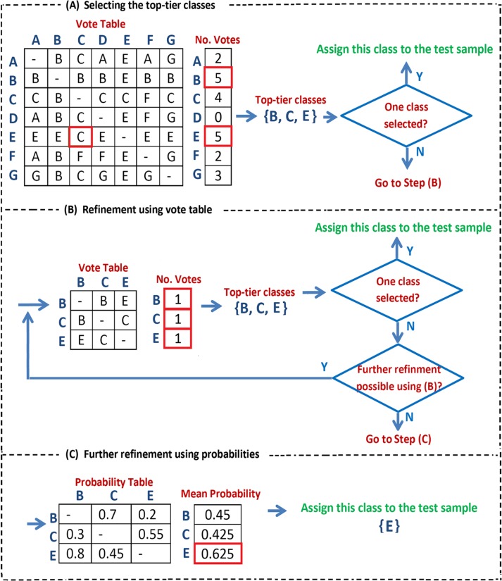
Based on the OvsO comparisons, we create a vote table where each binary classifier gives a vote for the predicted class and we count the votes received by each class. We then use the number of votes to select a set of top-tier classes that should be passed on the next level in the hierarchy. This top-tier set consists of: (1) any classes that get the maximum observed number of votes²⁹ and (2) any classes that beat a class with maximum number of votes in a one-to-one comparison. If we are at the lowest level in the hierarchy, then a single class among the top-tier classes must be assigned to the given test sample. To achieve that, we use the following rules to reduce the set of top-tier classes:

1. Recalculate the vote table using only the top-tier classes and only keep the classes that get the maximum number of observed votes in this new table. This step is repeated until no further classes are removed.

2. If more than 1 class is still left, then choose the class with the highest average probability score when looking at the OvsO comparisons between the remaining classes.

The explained classification process is summarized in Figure 1. In Step (A), all the classes are used and the classes with maximum number of votes are identified ({B, E}). Then, “C” which beats one of the classes with maximum number of votes (“B”) is added to the selected set of top-tier classes. In Step (B), refinement is applied to {B, C, E}: the voting table corresponding to the given set is made followed by selecting the closest cancer types using the same rules applied in Step A. This process continues iteratively until the size of the selected set of top-tier classes cannot be further reduced using these rules. In this example it is not possible to refine {B, C, E}. Therefore, the probability table calculated in the OvsO comparisons between all the pairs of {B, C, E} is taken into account in Step (C). Finally, the class with the maximum mean probability (“E”) is assigned to the given test sample. In the aforementioned algorithm, whenever only 1 class is selected at Step (A) or (B), it is the end of the classification process and that class is assigned to the sample.

Figure 1.

The proposed process of the classification using OvsO. Step A: selecting the top-tier classes with maximum number of votes ({B, E}) together with “C” which beats “B.” Step B: further refinement is applied on {B, C, E}. This process continues iteratively until the size of the selected set of top-tier cancers cannot be further reduced. Step C: based on the probability table, “E” with the maximum mean probability is assigned to the given sample.

To integrate multi-omics data, the refinement process (steps (B) and (C)) is accomplished using a second feature space. As the set of top-tier classes might be more separable in the new space, this tie-breaking classifier can improve the performance of classification. The other important advantage of the proposed hierarchical method is that no optimization technique is required for learning the combination of 2 layers, and the training cohorts of different omics types can be different.

Results and Discussion

To evaluate the performance of the proposed classifier, we first examine the results of classification using a single type of omics features before we test the classification using multi-omics data. The same test cohort is used for all the examinations.

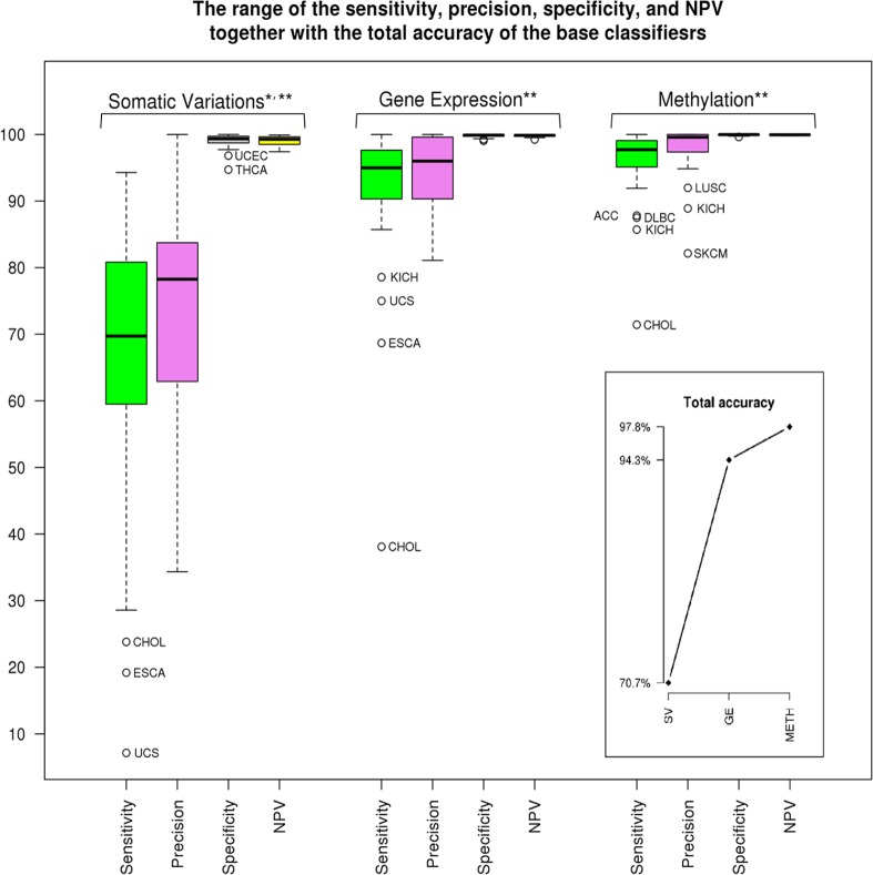
Total accuracy together with the range of specificity, sensitivity, precision, and negative predictive value (NPV)³⁰ within a single feature space by using the OvsO rules are given in Figure 2. Total accuracy is the fraction of correctly classified subjects to the size of the test cohort. The average of each of the quantities of specificity, sensitivity, precision, and NPV across cancer types is also provided (P < 10⁻¹⁶). The confidence level of 95% is used to compute P-values. Gene expression and METH data types hold tissue-specific information together with alterations associated with the cancerous disease.^31,32 Therefore, by applying an appropriate machine learning method, high accuracy of cancer classification is expected from these profiles. In this study, total accuracy of GE and METH is 94.3% and 97.8%, respectively. When we look at the cancer types with low classification sensitivity, we see that cholangiocarcinoma (CHOL) is not classified well in comparison with most of the other cancer types by using SV, GE, and METH. (Clinically as well as pathologically, CHOL may also be very difficult to diagnose.³³ Quite often CHOL is reported as the carcinoma of the upper gastrointestinal tract, including bile duct.). Esophageal carcinoma (ESCA) and uterine carcinosarcoma (UCS) have the same problem within SV and GE, whereas kidney chromophobe (KICH) has low sensitivity using GE and METH. Therefore, ESCA, UCS, and KICH have the chance for correct classification using another feature space, which is not available for CHOL.

Figure 2.

Total accuracy and the range of specificity, sensitivity, precision, and NPV related to each of the omics data. *P < 10⁻¹⁶, the average of sensitivity and precision of SV. **P < 10⁻²⁸ for the rest of quantities. NPV indicates negative predictive value; SV, somatic variant.

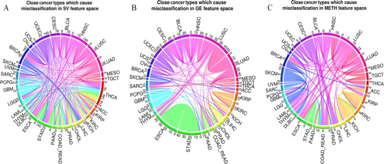
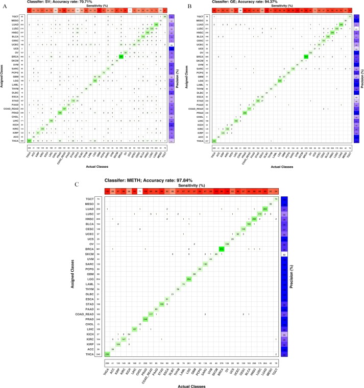
Appendix Figure B2 shows the confusion matrices of each of the feature spaces. As expected, SV has higher error rate in comparison with the other omics data. The number of misclassified pairs of each of the single omics data is represented in chord diagrams in Figure 3. The abbreviations of the cancer names are given in Table 1. When using GE, cancers belonging to the pan-squamous (LUSC, HNSC, CESC, ESCA, and BLCA)¹⁸ have more overlap with each other in comparison with SV and METH. However, the number of misclassified samples for the pair of STAD and ESCA is considerable for GE. Pan-kidney (KIRC, KIRP, and KICH)¹⁸ includes close cancer types using METH and GE. ACC and KIRC is another overlapped pair in METH feature space. Cancers associated with digestive organs (ESCA, COAD-READ, STAD, LIHC, CHOL, and PAAD) have more overlap with each other when applying GE compared to SV and METH. Misclassified samples between cancer types related to the digestive organs and pan-squamous are notable when SV and METH are used. In addition, CHOL and COAD-READ are both close to BRCA when using METH. In the case of SV, LIHC and BRCA are identified as close cancer types. LGG and GBM have overlap when using SV and GE. The classification performance of SKCM is better for GE and SV in comparison with METH. Pan-GYN (BRCA, OV, UCEC, and UCS)¹⁸ has important cancer types, which overlap with each other using GE. These cancers have other overlaps with pan-squamous and those related to the digestive organs when METH and SV are used.

Figure 3.

Number of misclassified pairs using single omics data. The weight of the edges shows how significant is the overlap of close cancer types using (A) SV, (B) GE, and (C) METH. For example, 27 samples of STAD are misclassified as ESCA and 13 samples of ESCA are classified as STAD by using GE. As a result, the number of misclassified pairs <STAD, ESCA> using GE is 40, which is illustrated as the weight of the edge between STAD and ESCA. ESCA indicates esophageal carcinoma; GE, gene expression; METH, methylation; NPV, negative predictive value; STAD, stomach adenocarcinoma; SV, somatic variant.

As seen in Figure 3, the overlap of the cancer types is not the same when different omics data are used. As a result, to improve the accuracy of using single omics data, we apply our proposed hierarchical setting. By referring to the type of the features used for these classifiers, the hierarchy is named. For example, in the case of “GE-SV,” GE is used for the base classifier and SV for the tie-breaker. The number of misclassified and correctly classified samples by the proposed method is given in the bar charts of Figure 4. In each figure, the left plot demonstrates total accuracy and number of samples classified by the base classifier and tie-breaker. Number and accuracy of classification of the samples analyzed by the tie-breaker are given in the right plot.

Figure 4.

Accuracy of classification and number of misclassified/correctly classified samples by the base classifier and tie-breaker. (A) to (C) are associated with the classification of the test cohort of TCGA. In these figures, SV, GE, and METH are used for the base classifier, accordingly. (D) illustrates the classification result for MET500 with the base classifier of GE and SV in the second layer. At the left plot of each figure, the total number of samples which are misclassified/correctly classified is depicted. The upper part of these plots indicated by dashed lines show the samples which are further examined. Total accuracies using single omics data and in combination with the other features are given, respectively. In the right plot of each figure, further examined samples and corresponding accuracies are given. Misclassified samples are categorized into 2 groups: “correction possible” and “correction not possible.” In the case of former, the actual class of a test sample is selected for further analysis. However, for the latter case, the actual class is not given in the set of top-tier cancers. GE indicates gene expression; METH, methylation; SV, somatic variant; TCGA, The Cancer Genome Atlas.

Misclassified samples by the tie-breaker are divided into 2 groups: “misclassified by tie-breaker, correction possible” and “misclassified by tie-breaker, correction not possible.” The difference between these 2 groups is related to the set of top-tier classes suggested by the base classifier. If the actual class of a test sample is not given in the selected set of cancers, then there is no possibility for the tie-breaker to correctly classify it. These samples are labeled as “correction not possible.” Otherwise, there is possibility for correctly classify that sample (ie, “correction possible”).

In all the tested hierarchies, the accuracy of the base classifier improves by using another omics data. As it is expected, using a highly accurate classifier as a tie-breaker results in less misclassified samples. By applying SV-METH, an additional 40.08% of the further examined samples are correctly classified. In the combination of GE-METH, METH can identify all the samples with the possibility of correction. By applying the most accurate classifiers (METH-GE in this study), 98.04% of the test samples are correctly classified. In the aforementioned combination, METH (used for the base classifier) presents the most accurate results among the single omics data. Therefore, as a base classifier, it increases the number of correctly classified samples which do not need to be examined further (depicted in blue in Figure 4). In addition, it suggests promising sets of top-tier cancers to the next layer to decrease the number of samples indicated as “misclassified by tie-breaker, correction not possible.” In the combination of METH-GE, GE is the second-most accurate single omics data. When it is used for further analysis of the samples, it reduces the error of classification as a tie-breaker.

The MET500 data set does not include methylation data. As a result, GE and SV are used to classify the primary site of the cancers. As the performance of classification using GE is better than SV, it is applied as the base classifier. Figure 4D illustrates the number of samples of MET500 and accuracy of classification by using GE and GE-SV. Although the transcriptome profiles and mutational burdens of metastatic cancers are different from primary tumors,²⁵ GE-SV classify MET500 with an accuracy of 82.17%. By applying the suggested algorithm, number of further examined samples is 8 (out of 185). Although the performance of SV is lower than GE, it can still improve the accuracy of classification as a tie-breaker.

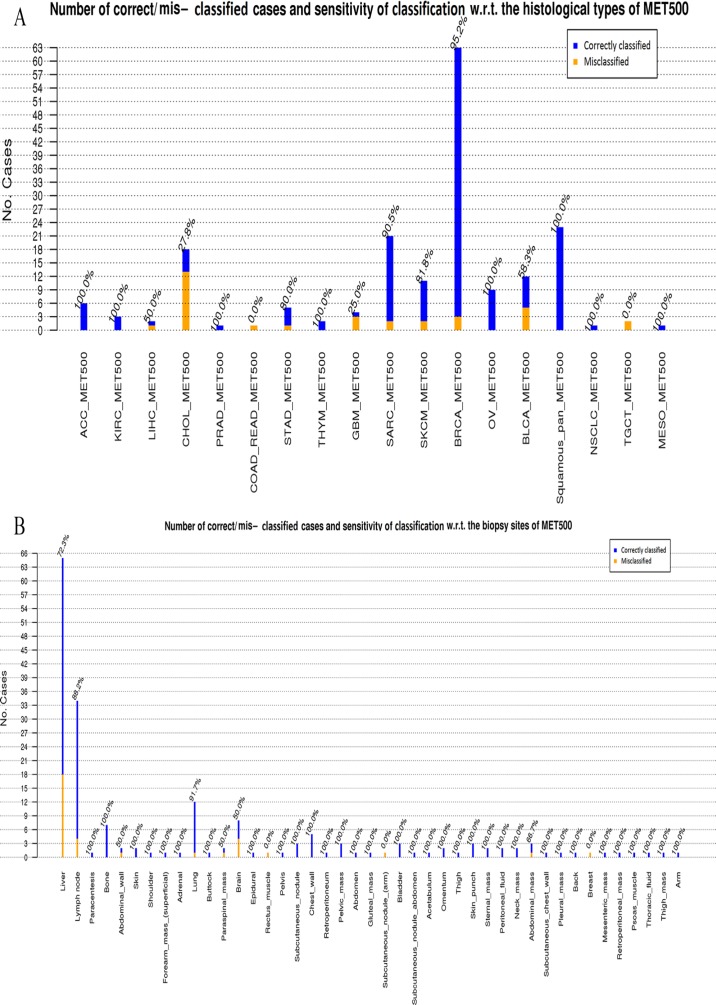
Appendix Figure B3 shows the bar charts of the number of correct/mis-classified cases together with the sensitivity of classification for MET500 using GE-SV by considering (1) histological type and (2) biopsy site of the subjects. BRCA_MET500, squamous_pan_MET500, and SARC_MET500 are the most prevalent histological types, and these are classified with a sensitivity of 95.2%, 100%, and 90.5%, respectively. However, only 27.8% of CHOL_MET500 are classified correctly. As this cancer type is poorly diagnosed using different multi-omics data of TCGA (Figure 2 and Appendix Figure B2), our classifier is not capable of correctly identifying CHOL. In the case of the biopsy site, most of the misclassified samples are taken from liver (sensitivity of diagnosis 72.3%). The other main biopsy sites are lymph node, lung, brain, and bone with sensitivity of 88.2%, 91.7%, 50%, and 100%, respectively.

Figure 5 shows the biopsy site, histological type, and the assigned cancer type related to the misclassified samples after applying GE-SV classifier. 50% of the misclassified samples with the biopsy site of the liver are identified as CHOL_MET500 (9 out of 18). There are 4 samples of BLCA_MET500 which are classified as CESC and LUSC which makes sense as BLCA, CESC, and LUSC are all squamous cell cancers, and these are known to show high degrees of molecular similarity.¹⁸ In addition, 3 out of 4 of the misclassified GBM samples are classified as LGG and these are both tumors of the brain, so in these cases we at least get the organ of the tumor right.

Figure 5.

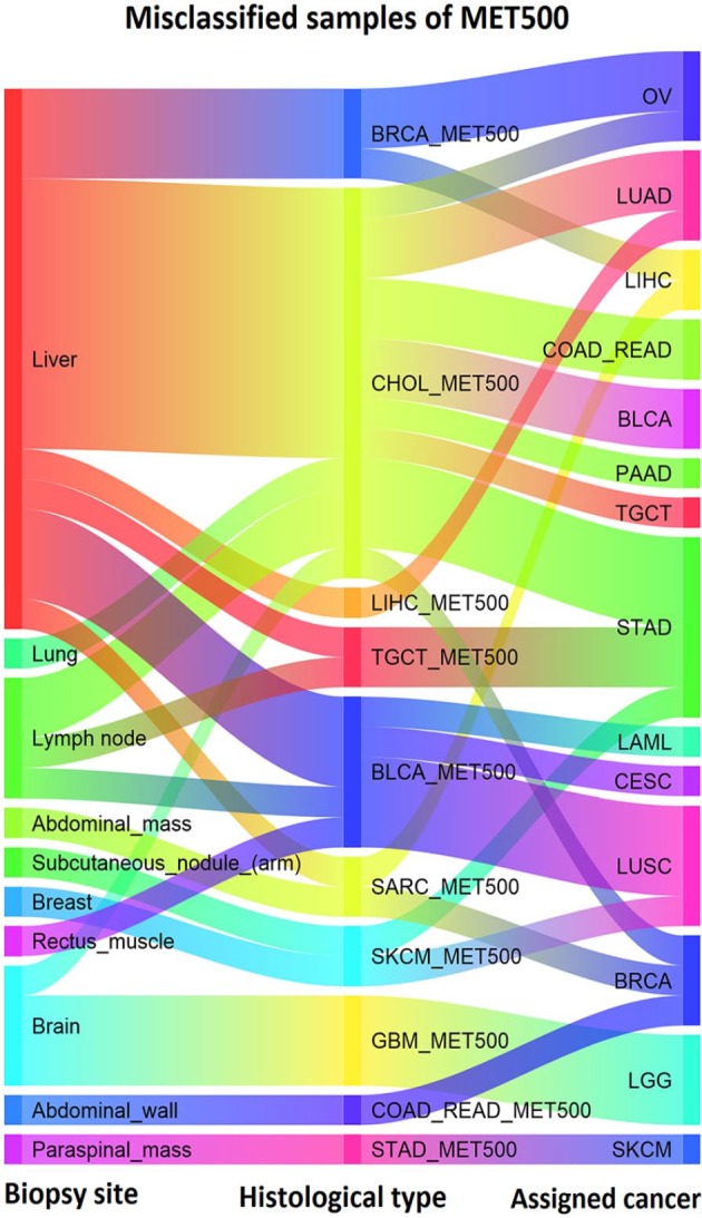
Biopsy site, histological type and the assigned cancer type of the misclassified samples using GE-SV. GE indicates gene expression; SV, somatic variant.

Conclusions

In this study, a new hierarchical method for CUP classification using multi-omics data is proposed, in which classification is accomplished by applying one of the omics data as a base classifier. If a high certainty answer cannot be provided using the base, another type of omics data is used as a tie-breaker.

We show that in any combination of omics data, the accuracy of the base classifier is improved by the addition of another feature space. The most effective combination for the hierarchical model is achieved by using the most informative data for the base classifier and the second most informative one for the tie-breaker, which corresponds to first classifying using methylation data and then using GE data for the tie-breaker. The main advantage of using the most informative omics data is decreasing the number of misclassified samples for which further examination is not required. In addition, it increases the possibility of suggesting a promising set of cancers to the next layer. The second-most accurate classifier reduces the error of classification as a tie-breaker.

During the learning process, a separating hyperplane is estimated for each pair of cancer types using each of the omics data. As a result, an arbitrary set of suggested cancers can be examined independently of the others. In addition, different training cohorts can be used for each of the omics types. As BLR is applied to learn the separating hyperplanes, the probability of a given sample belonging to a certain cancer type is available. This feature, together with the advantage of applying independent separating hyperplanes, is used for refinement of the set of top-tier classes using tie-breaker.

In this study, the tested omics data include methylome, transcriptome, simple nucleotide variations, and CNVs from TCGA. Methylation-gene expression was the best combination, but as methylation data are not present in the MET500 dataset, we instead use the GE-SV classifier for this validation data set. The combination of GE-SV classifies MET500 with an accuracy of 82.17%.

In conclusion, our results on TCGA and metastatic samples show that using multi-omics data might be useful in the clinical setting to improve the diagnosis of the patients with CUP. The proposed hierarchical method can easily be extended to include other types of data (eg, proteomics/metabolomics or histological images). As the method is not dependent on having the same type of data for all samples, it is feasible to include other types of data without reducing number of training samples drastically. The strategy used in the proposed hierarchical classifier is not limited to the context of bioinformatics but could in principle be used for other classification problems.

Appendix A

Probabilities computed using binomial logistic regression

By applying binomial logistic regression (BLR), the probabilities of belonging to the classes can be computed. For the samples which are far from the separating hyperplane, the likelihood corresponding to the winner class is more than those near to it. The following equations are applied to compute the probabilities of belonging to the classes²⁸

$$\mathrm{Pr}\left(G=c_1|x\right)=\frac{1}{1+{\mathrm{e}}^{-\left({\beta }_0+x^T\beta \right)}}$$

$$\mathrm{Pr}\left(G=c_2|x\right)=\frac{1}{1+{\mathrm{e}}^{+\left({\beta }_0+x^T\beta \right)}}=1-\mathrm{Pr}\left(G=c_1|x\right)$$

where $G\in \{c_1,c_2\}$ represents the label of the suggested class, $x$ is the feature vector of the given sample, and $\beta$ s are the estimated parameters of the biclassifier.

Appendix B

Figure B1.

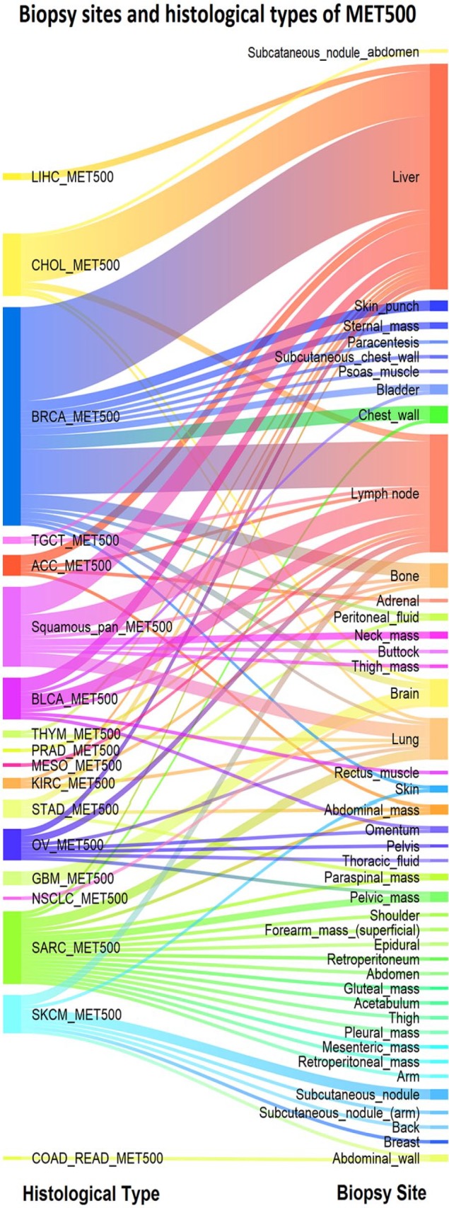
Histological type and the biopsy site for the metastatic samples of MET500. The most frequent biopsy sites are liver, lymph node, and lung with 65, 34, and 12 cases, respectively. Prevalent histological types are BRCA_MET500, Squamouse-pan_MET500, SARC_MET500, and CHOL_MET500 with 63, 23, 21, and 18 samples. SARC_MET500 and SKCM_MET500 are associated with a wide range of biopsy sites.

Figure B2.

(A) to (C) Confusion matrices of single classifiers: SV, GE, and METH. The zero values of the matrices are shown as blank. GE indicates gene expression; METH, methylation; SV, somatic variant.

Figure B3.

The bar chart and sensitivity of classification for MET500 with respect to (A) histological type and (B) biopsy site of the subjects.

Appendix C

Table C1.

Data portals and the date of downloads of the used datasets.

Dataset	Date of download	Source
GE	November 16, 2016	TCGA project (GDC data portal: https://portal.gdc.cancer.gov)
SV	January 20, 2017	TCGA project (GDC data portal: https://portal.gdc.cancer.gov)
METH	May 18, 2018	http://firebrowse.org/ provided by TCGA project; filenames: *.meth.by_mean.data.txt
COSMIC	January 12, 2017	Catalog of the Somatic Mutations in Cancer: https://cancer.sanger.ac.uk/cosmic
GTEx	December 2016	dbGaP (The Database of Genotypes and Phenotypes: https://www.ncbi.nlm.nih.gov/gap)
MET500	January 4, 2018	dbGaP (The Database of Genotypes and Phenotypes: https://www.ncbi.nlm.nih.gov/gap)

Abbreviations: COSMIC, Catalogue of Somatic Mutations in Cancer; GE, gene expression; METH, methylation; NPV, negative predictive value; SV, somatic variant; TCGA, The Cancer Genome Atlas.

Table C2.

Actual histological name used in MET500 and the corresponding abbreviation used in this study.

Abbreviation	Histological types presented in MET500
NSCLC_MET500	NSCLC (non-small cell lung cancer)
PRAD_MET500	Poorly_differentiated_prostate_carcinoma_with_focal_small_cell/neuroendocrine
BRCA_MET500	Breast cancer Ductal_carcinoma, Ductal_/_lobular_carcinoma, Lobular_carcinoma Carcinoma_with_apocrine_features Poorly_differentiated_carcinoma_with_lobular_features Mixed_ductal_and_lobular_carcinoma Ductal_and_lobular_carcinoma
SARC_MET500	Dediferentiated_liposarcoma, Pleomorphic_sarcoma Myxoid/round_cell_liposarcoma High_grade_sarcoma, Undifferentiated_pleomorphic_sarcoma Pleomorphic_undifferentiated_sarcoma, Leiomyosarcoma Synovial_sarcoma
CHOL_MET500	Extra-hepatic_cholangiocarcinoma Cholangiocarcinoma
THYM_MET500	Thymoma Thymic_squamous_carcinoma
ACC_MET500	Adrenocortical_carcinoma
KIRC_MET500	Renal_cell_carcinoma
LIHC_MET500	Hepatocellular_carcinoma
COAD_READ_MET500	Colorectal_adenocarcinoma
STAD_MET500	Signet_ring_adenocarcinoma Gastrointestinal_stromal_tumor
OV_MET500	Serous_carcinoma Serous_papillary_carcinoma Papillary_serous_carcinoma
BLCA_MET500	Urothelial_carcinoma Urothelial_carcinoma_with_squamous_differentiation
Squamous_pan_MET500	Poorly_differentiated_squamous_carcinoma Squamous_cell_carcinoma
TGCT_MET500	Non-seminomatous_germ_cell_tumor
GBM_MET500	Glioblastoma
SKCM_MET500	Melanoma
MESO_MET500	Mesothelioma

References

- 1. Oien KA. Pathologic evaluation of unknown primary cancer. Semin Oncol. 2009;36:8-37. [DOI] [PubMed] [Google Scholar]
- 2. Fizazi K, Greco FA, Pavlidis N, Daugaard G, Oien K, Pentheroudakis G; ESMO Guidelines Committee. Cancers of unknown primary site: ESMO clinical practice guidelines for diagnosis, treatment and follow-up. Ann Oncol. 2015;26:133-138. [DOI] [PubMed] [Google Scholar]
- 3. Dietlein F, Eschner W. Inferring primary tumor sites from mutation spectra: a meta-analysis of histology-specific aberrations in cancer-derived cell lines. Hum Mol Genet. 2014;23:1527-1537. [DOI] [PubMed] [Google Scholar]
- 4. Amar D, Izraeli S, Shamir R. Utilizing somatic mutation data from numerous studies for cancer research: proof of concept and applications. Oncogene. 2017;36:3375-3383. [DOI] [PMC free article] [PubMed] [Google Scholar]
- 5. Marquard AM, Birkbak NJ, Thomas CE, et al. TumorTracer: a method to identify the tissue of origin from the somatic mutations of a tumor specimen. BMC Med Genomics. 2015;8:58. [DOI] [PMC free article] [PubMed] [Google Scholar]
- 6. Soh KP, Szczurek E, Sakoparnig TH, Beerenwinkel N. Predicting cancer type from tumour DNA signatures. Genome Med. 2017;9:104. [DOI] [PMC free article] [PubMed] [Google Scholar]
- 7. Schölkopf B, Smola AJ. Learning With Kernels. Cambridge, MA: MIT Press; 2002. [Google Scholar]
- 8. Bailey MH, Tokheim C, Porta-Pardo E, et al. Comprehensive characterization of cancer driver genes and mutations. Cell. 2018;173:371-385. [DOI] [PMC free article] [PubMed] [Google Scholar]
- 9. Alexandrov LB, Nik-Zainal S, Wedge DC, et al. Signatures of mutational processes in human cancer. Nature. 2013;500:415-421. [DOI] [PMC free article] [PubMed] [Google Scholar]
- 10. Moran S, Martinez-Cardús A, Boussios S, Esteller M. Precision medicine based on epigenomics: the paradigm of carcinoma of unknown primary. Nat Rev Clin Oncol. 2017;14:682-694. [DOI] [PubMed] [Google Scholar]
- 11. Tothill RW, Kowalczyk A, Rischin D, et al. An expression-based site of origin diagnostic method designed for clinical application to cancer of unknown origin. Cancer Res. 2005;65:4031-4040. [DOI] [PubMed] [Google Scholar]
- 12. Van Laar RK, Ma XJ, de Jong D, et al. Implementation of a novel microarray-based diagnostic test for cancer of unknown primary. Int J Cancer. 2009;125:1390-1397. [DOI] [PubMed] [Google Scholar]
- 13. Varadhachary GR, Spector Y, Abbruzzese JL, et al. Prospective gene signature study using microRNA to identify the tissue of origin in patients with carcinoma of unknown primary. Clin Cancer Res. 2011;17:4063-4070. [DOI] [PubMed] [Google Scholar]
- 14. Galea D, Inglese P, Cammack L, et al. Translational utility of a hierarchical classification strategy in biomolecular data analytics. Sci Rep. 2017;7:14981. [DOI] [PMC free article] [PubMed] [Google Scholar]
- 15. Sondergaard D, Nielsen S, Pedersen CNS, Besenbacher S. Prediction of primary tumors in cancers of unknown primary. J Integr Bioinform. 2017;14:20170013. [DOI] [PMC free article] [PubMed] [Google Scholar]
- 16. Breiman L. Random forests. Mach Learn. 2001;45:5-32. [Google Scholar]
- 17. Moran S, Martínez-Cardús A, Sayols S, et al. Epigenetic profiling to classify cancer of unknown primary: a multicentre, retrospective analysis. Lancet Oncol. 2016;17:1386-1395. [DOI] [PubMed] [Google Scholar]
- 18. Hoadley KA, Yau C, Hinoue T, et al. Cell-of-origin patterns dominate the molecular classification of 10,000 tumors from 33 types of cancer. Cell. 2018;173:291.e6-304.e6. [DOI] [PMC free article] [PubMed] [Google Scholar]
- 19. Bishop CM. Pattern Recognition and Machine Learning. Berlin, Germany: Springer; 2006. [Google Scholar]
- 20. Vapnik VN. Statistical Learning Theory. Hoboken, NJ: John Wiley and Sons; 1998. [Google Scholar]
- 21. Jain A, Nandakumar K, Ross A. Score normalization in multimodal biometric systems. Pattern Recogn. 2005;38:2270-2285. [Google Scholar]
- 22. Zhou ZH. Ensemble Methods: Foundations and Algorithms (Machine Learning & Pattern Recognition Series). London, England: Chapman & Hall/CRC; 2012. [Google Scholar]
- 23. Mitchell TM. Machine Learning. New York, NY: Mcgraw-Hill; 1997:175. [Google Scholar]
- 24. Ciriello G, Miller ML, Aksoy BA, Senbabaoglu Y, Schultz N, Sander C. Emerging landscape of oncogenic signatures across human cancers. Nat Genet. 2013;45:1127-1133. [DOI] [PMC free article] [PubMed] [Google Scholar]
- 25. Robinson DR, Wu YM, Lonigro RJ, et al. Integrative clinical genomics of metastatic cancer. Nature. 2017;548:297-303. [DOI] [PMC free article] [PubMed] [Google Scholar]
- 26. Gosink MM, Petrie HT, Tsinoremas NF. Electronically subtracting expression patterns from a mixed cell population. Bioinformatics. 2007;23:3328-3334. [DOI] [PubMed] [Google Scholar]
- 27. GTEx Consortium. Genetic effects on gene expression across human tissues. Nature. 2017;550:204-213. [DOI] [PMC free article] [PubMed] [Google Scholar]
- 28. Friedman J, Hastie T, Tibshirani R. Regularization paths for generalized linear models via coordinate descent. J Stat Softw. 2010;33:1-22. [PMC free article] [PubMed] [Google Scholar]
- 29. Wang Z, Xue X. Multi-Class Support Vector Machine. Berlin, Germany: Springer; 2014. [Google Scholar]
- 30. Beleites C, Salzer R, Sergo V. Validation of soft classification models using partial class memberships: an extended concept of sensitivity & co. applied to grading of astrocytoma tissues. Chemometr Intell Lab Syst. 2013;122:12-22. [Google Scholar]
- 31. Beckerman M. Cellular Signaling in Health and Disease. Berlin, Germany: Springer; 2009. [Google Scholar]
- 32. Weber GF. Molecular Mechanisms of Cancer. Berlin, Germany: Springer; 2007. [Google Scholar]
- 33. Razumilava N, Gores GJ. Classification, diagnosis, and management of cholangiocarcinoma. Clin Gastroenterol Hepatol. 2013;11:13.e1-21.e1; quiz e3-e4. [DOI] [PMC free article] [PubMed] [Google Scholar]