Detection and Classification of Novel Renal Histologic Phenotypes Using Deep Neural Networks

Abstract

With the advent and increased accessibility of deep neural networks (DNNs), complex properties of histologic images can be rigorously and reproducibly quantified. We used DNN-based transfer learning to analyze histologic images of periodic acid-Schiff–stained renal sections from a cohort of mice with different genotypes. We demonstrate that DNN-based machine learning has strong generalization performance on multiple histologic image processing tasks. The neural network extracted quantitative image features and used them as classifiers to look for differences between mice of different genotypes. Excellent performance was observed at segmenting glomeruli from non-glomerular structure and subsequently predicting the genotype of the animal on the basis of glomerular quantitative image features. The DNN-based genotype classifications highly correlate with mesangial matrix expansion scored by a pathologist (R.E.C.), which differed in these animals. In addition, by analyzing non-glomeruli images, the neural network identified novel histologic features that differed by genotype, including the presence of vacuoles, nuclear count, and proximal tubule brush border integrity, which was validated with immunohistologic staining. These features were not identified in systematic pathologic examination. Our study demonstrates the power of DNNs to extract biologically relevant phenotypes and serve as a platform for discovering novel phenotypes. These results highlight the synergistic possibilities for pathologists and DNNs to radically scale up our ability to generate novel mechanistic hypotheses in disease.

Kidney dysfunction is associated with many histologic changes encompassing glomerular, vascular, and tubulointerstitial diseases.¹ For example, although diabetic nephropathy can result in lesions, such as glomerular hypertrophy, hyperplasia, mesangial matrix expansion (MME), hypercellularity, and glomerular basement membrane thickening, it can also alter the histology of the Bowman space, arterioles, arteries, tubules, and the interstitium.² Current approaches to measuring histologic changes in the kidney are difficult to quantify and have a low throughput. Many alterations, such as MME in the glomerulus, require a trained observer to manually segment histologic images and subjectively score the extent of MME.³ Therefore, trained pathologists are often only able to score a limited number of phenotypes on a limited number of slides.

Traditionally, histologic scoring falls into two broad categories: automatic scoring, using relatively simple measures, such as staining intensity per unit area, that are mathematically rigorous, but can be biologically imprecise⁴; and complex heuristic scoring, using biologically precise patterns, such as loss of capillary lumen, that are detectable by trained human observers, but are more difficult to quantify.⁵ In the latter case, pathologists use subjective scoring systems with a low throughput. Moreover, both strategies require an a priori specification of the relevant image features to quantify, which leaves no room for the discovery of novel phenotypes.

Histologic structures are complex and can have immense variability. Until recently, this variability has been a barrier to automated analysis. The ability to rigorously quantify multiple complex image properties with high throughput and integrate them into a judgment about morphologic state is an unresolved computer vision problem. However, advances in computer vision, called deep neural networks (DNNs), have radically expanded the properties of complex images that can be quantified. Humans can readily distinguish, for example, a cat from a dog, but training a computer at this task remained a problem until the development of DNNs.⁶ DNNs are trained using a data-driven strategy called deep learning to identify complex features from tens of millions of natural images representing thousands of labeled objects.⁶ DNNs transform raw images into a high-dimensional signature of abstract quantitative image features (QIFs) that quantify complex image properties, such as textural patterns. More important, these QIFs are transferable among image classification problems, allowing a DNN trained on natural images to be transferred to other settings, a process called transfer learning.⁷ Recent work has demonstrated that DNNs achieve human-expert level performance at natural and biomedical image classification tasks.7, 8 These DNNs can substantially augment histologic scoring and enable more robust quantitative analysis.

In this work, we demonstrate the power of DNNs to identify and quantify specific features in renal tissue structures and discover novel histopathologic features that are missed by human observation. Transfer learning was applied to dissect complex histopathologies of the kidney as a proof of principle that DNN analysis is a mature discovery platform for histologic analysis. DNNs were used to automatically segment glomeruli in histologic images obtained by standard bright-field light microscopy using the high-dimensional DNN outputs. This could be done in a robust manner, processing each slide in approximately 40 minutes using the Vermont Advanced Computing Center. It was further shown that the DNN-based QIFs are relevant to histopathology by using them to predict the genotype of mice that are either wild type (WT) or knockout (KO) for the Far2 gene.

Materials and Methods

Animals and Samples

B6N(Cg)-Far2^{tm2a(KOMP)Wtsi}/2J male mice were generated by the Knockout Mouse Phenotyping Program (KOMP2) at The Jackson Laboratory (Bar Harbor, ME) using C57BL/6N-derived embryonic stem cells provided by the International Knockout Mouse Consortium, as previously described.⁹ At 6, 12, and 18 months of age, animals [wild-type, heterozygous (HET), and knockout mice] were euthanized and kidneys were collected. Left kidneys were cut in half along the sagittal plane and placed in 4% paraformaldehyde in phosphate-buffered saline for 24 hours at room temperature. The kidneys were embedded in paraffin, divided into section (4 μm thick), stained with periodic acid-Schiff, and counterstained with hematoxylin using a Leica autostainer XL ST5020 (Leica Biosystems, Buffalo Grove, IL). All 90 slides were scanned at 40× objective using a Hammamatsu nanozoomer 2.0HT digital slide scanner (Hammamatsu, Bridgewater, NJ). Bright-field individual Tagged Image File Format (TIFF) images were obtained using the NDPtools macro.¹⁰ Animal experiments were approved by the Institutional Animal Care and Use Committee.

DNN Feature Extraction

To extract quantitative image features, the AlexNet DNN,⁵ which is available through the MATLAB Deep Learning Toolbox (Mathworks, Natick, MA), was used. AlexNet uses a cascade of mathematical transformations (image filtering, averaging, and rectified linear thresholding) to transform the raw input image into a series of numbers that quantify different patterns.¹¹ These transformations are arranged in a sequence of 26 layers. The lowest layers correspond to primitive features, such as boundaries between light and dark, whereas the higher layers correspond to progressively more abstract features, such as textures and patterns. AlexNet was trained to classify images into one of the 1000 classes (eg, boat or cat), representing a wide spectrum of natural images. However, higher-layer intermediate features capture complex structures that are present in many image classes, and not just natural images. For this study, features were extracted from the 17th layer of AlexNet, called fully connected layer 6, which reports 4096 distinct quantitative features. AlexNet has a fixed input size of 227 × 227 pixels (px), where 1 px corresponds to 226 nm of tissue in our images. Therefore, AlexNet was applied to 227 × 227-px image patches to obtain 4096 features per patch that were used to train subsequent classifiers. Feature values were standardized (mean subtracted and normalized to SD) and subsequently used by support vector machine (SVM) classifiers. All feature extraction was performed on the Vermont Advanced Computing Core's central processing unit (CPU) cluster via torque server submission.

SVM Training

All SVM classifiers were trained with the MATLAB Statistics and Machine Learning Toolbox (Mathworks, Natick, MA). Kernel SVM classifiers, which are nonlinear learning algorithms that have three hyperparameters (box constraint, kernel scale, and cost), were used. The box constraint parameter controls how much a model penalizes an incorrect prediction in the training data. The kernel radius determines how much the model extrapolates a given training data points class to nearby points. The cost parameter controls how much the model penalizes a false positive relative to a false negative. All hyperparameters were fit using MATLAB's built-in optimization in which many putative models are built with various parameters and the resulting accuracies are compared using cross validation (Mathworks). For the segmentation pipeline, a gaussian kernel was used with a kernel scale of 150 and a box constraint of 377. A 5-to-1 cost penalty of false negatives to false positives was used, as false positives were readily identified in post-processing (see below). For the genotype comparisons, a polynomial kernel was used, which had an additional hyperparameter, polynomial order. Polynomial order was also selected automatically using MATLAB's built-in tools, and polynomial orders of three and two were selected for the glomerular and tubular analysis, respectively. For reproducibility, all computations were performed with the default random number generator seed, and all analysis code is available on GitHub (https://github.com/TheJacksonLaboratory/ImageFeature, last accessed March 12, 2019).

SVM models produce a final classification as well as a confidence score, which quantifies how strongly the classifier weighs the evidence for either class. SVM model performance was visualized using a receiver operating characteristic curve, which plots the true-positive rate versus the false-positive rate as a function of the confidence score. Ideally, the receiver operating characteristic curve should climb steeply to a high true-positive rate (near 1) at low false-positive rate (near 0) before leveling off and reaching the point (1, 1) in the upper right. Random guessing corresponds to a 45-degree line. Receiver operating characteristic curves shown use a set of images not included in the training data specifically held out for validation.

Automatic Segmentation of Glomeruli Using Support Vector Machines

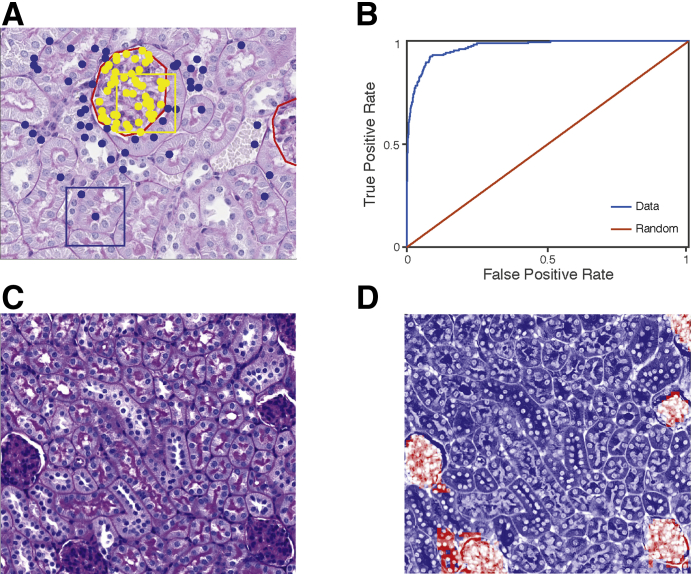
Our strategy to automatically segment glomeruli was as follows. After intensity normalizing all images using the MATLAB histeq function to account for differing stain intensities between sections, an SVM was trained to classify image patches according to whether their center pixel was inside or outside a glomerulus using the 4096 AlexNet features for that image patch (Figure 1A). For training data, glomeruli were hand segmented in eight training images and 100 image patches sampled from each image balanced between glomerular patches and tubule patches (Figure 1A). One image was held out for testing. To enrich the training data for edge cases close to a glomerular boundary, non-glomerular image patches inversely proportional to their distance from a glomerulus were sampled (Figure 1A), which ensured many training images that overlapped a glomerulus with center pixels on either side of the boundary.

Figure 1.

Glomerulus versus tubule classification strategy. A: To train a classifier to distinguish glomeruli, 100 image patches were sampled from eight hand-segmented example images (red lines). Fifty image patches per image whose center pixels were inside glomeruli (yellow dots) and 50 images patches whose center pixels were outside glomeruli (blue dots) were sampled. Yellow boxed area represents glomeruli patch, and blue boxed area represents non-glomeruli patch. B: The receiver operating characteristic curve for glomerular versus non-glomerular predictions shows strong generalization performance, achieving 92% true-positive rate for 10% false-positive rate. C and D: An example segmentation of a testing image shows that the model correctly identifies regions with glomeruli. Moreover, incorrectly classified pixels lie near the boundary of glomeruli, highlighting that the model correctly identifies contiguous regions containing glomeruli. Original magnification, ×40 (A, C, and D).

To automatically segment glomeruli in a new image, a two-step classification process was applied. First, a coarse-grained scan that sampled image patches in a square grid every 100 px (approximately 23 μm) was used, and the above classifier was used to classify patches into glomerulus versus tubule (Figure 2). The second step returns to the glomerulus predictions and samples more finely at 20 px (approximately 4.5 μm) to determine the exact boundary of the detected glomerulus (Figure 2). Final predictions were filtered to include only predicted points that formed contiguous regions of >35 pixels. This cutoff was selected by visual inspection of the distribution of region sizes on the training images (data not shown). Nearest-neighbor interpolation was used to extrapolate from the sampled predictions to a pixel-by-pixel mask of detected glomeruli within the image. Eight images were selected from the analysis set and hand sectioned to validate both the scanning method as well as transferability of the classifier.

Figure 2.

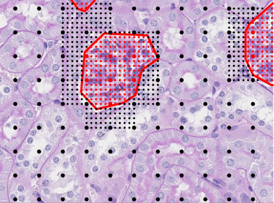
Glomerular segmentation strategy. To perform glomerular segmentation, the trained segmentation model was applied (Figure 1) to a square grid of points spaced 100 pixels (px) apart to classify grid points as inside glomeruli (large red dots) or outside glomeruli (large black dots). Human annotation of glomeruli is represented by red lines. For pixels classified as glomeruli, the segmenter returned to those locations to sample more finely at 20 px to determine glomerular boundaries (small dots). A final mask is generated through nearest-neighbor interpolation. Original magnification, ×40.

SVM Classification of Genotype Using AlexNet Features from Glomeruli

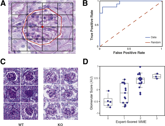
To classify glomeruli on the basis of genotype, 98 glomeruli (25 KO, 41 HET, and 32 WT) were analyzed from 45 kidney sections (17 KO, 16 HET, and 12 WT) from 17 animals (6 KO, 6 HET, and 5 WT). Because a typical glomerulus is larger than the fixed 227 × 227-px size for AlexNet, features were computed for nine overlapping patches around the center-of-mass pixel of the identified glomerulus (Figure 3A). These features were averaged together to produce a final 4096-dimensional feature vector for each glomerulus. An SVM was trained to distinguish KO from WT glomeruli using these averaged features. Seventy-eight glomeruli were held out to test the generalization performance of our classifier (Figure 3B).

Figure 3.

Classifying glomeruli by Far2 genotype. A: Glomeruli are typically larger than the 227 × 227-pixel squared input for AlexNet. To obtain features for classifying glomeruli by genotype, feature vectors obtained by taking nine image patches sampled in a grid around the center-of-mass pixel (center red dot) of the glomerulus were averaged. The human annotation of glomeruli is represented by a red line. B: The receiver operating characteristic curve for wild-type (WT) versus knockout (KO) predictions shows strong generalization performance, achieving an 87% true-positive rate at a 10% false-positive rate. C: The six most confidently predicted WT glomeruli show extensive mesangial matrix expansion (MME), whereas the six most confidently predicted KO glomeruli did not. D: The deep neural network (DNN)–based glomerulus score significantly correlates with MME scored by a pathologist (R² = 0.72; P = 9.03 × 10⁻⁸) in heterozygous glomeruli, which were not used to train the model, demonstrating that the DNN identified a known histopathology to classify genotype. Original magnification, ×40 (A and C). AU, arbitrary unit.

SVM Classification of Genotype Using AlexNet Features from Tubules

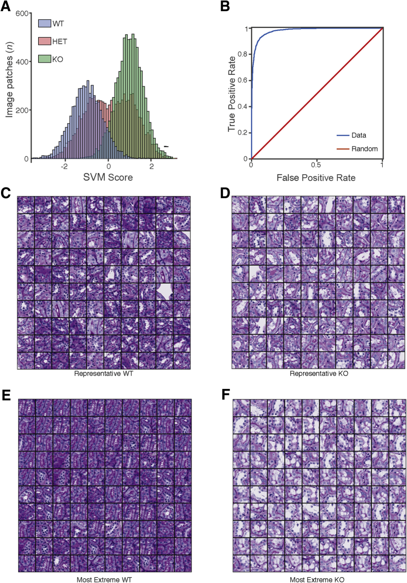
To classify tubules on the basis of genotype, 500 image patches of tubule structure were sampled from the same set of images as the glomeruli above. An SVM was trained to distinguish KO versus WT tubules on the basis of the 4096 features of each of these image patches. Thirty-five histologic slides were held out to test the generalization performance of our classifier (Figure 4B).

Figure 4.

Classifying tubules by Far2 genotype. A: Image patches of non-glomerular structure from wild-type (WT) and knockout (KO) animals were classified according to genotype. The Support Vector Machine (SVM) scores from the model in held-out testing data show that the model confidently distinguishes WT from KO and that heterozygotes (HETs) had an intermediate phenotype. B: The receiver operating characteristic curve for the model shows strong generalization performance, achieving a 95% true-positive rate at a 10% false-positive rate. C: To identify the histopathologic features distinguishing genotype, montages were generated. A total of 100 WT images around the mean of the SVM score (−1.01) showed a range of images with a minimum SVM score of -1.02 and a maximum SVM score of -0.99 (A, blue distributions, median values). D: A total of 100 KO image patches from around the mean of the SVM score (1.00) showed a range of images with a minimum SVM score of 0.99 and a maximum SVM score of 1.01 (A, green distributions, median values). E: Montages were also generated. A total of 100 WT images with the most extreme SVM score are shown (average value, -2.88; minimum SVM score, -3.89; and maximum SVM score, -2.52). F: A total of 100 KO image patches with the highest SVM scores are shown (average, 2.64; minimum SVM score, 2.45; and maximum SVM score, 3.38). These images suggest differences in vacuolization and nuclear counts around the tubule. Original magnification, ×40 (C–F).

Pathologic Scoring of Glomeruli

Mesangial matrix expansion was assessed in the glomeruli, as previously described.¹² Briefly, renal pathologists evaluated 50 glomeruli per animal to score the mesangial matrix [0 indicates no MME; 1, increase in extracellular material (mesangial matrix) and/or cellularity (mesangioproliferation) such that the width of the intercapillary space exceeds two mesangial cell nuclei but does not exceed the mean area of the glomerular capillary lumen; 2, the expanded mesangial area exceeds the mean area of a capillary lumen and often distorts/compresses the capillaries (microaneurysms are sometimes observed); and 3, the mesangium is expanded and/or sclerosed to such extent that capillary lumens are completely collapsed and can no longer be distinguished (collapsing glomerulosclerosis and completely sclerosed obsolescent glomeruli also fall into this category)].

Pathologic Scoring of Tubules

Vacuolization was quantified using ImageJ software version 1.51h (NIH, Bethesda, MD; http://imagej.nih.gov/ij) on representative and extreme image patches classified in the Support Vector Machine (Figure 5). Briefly, a measure of the image covered by tissue is taken by preforming a blur on the images and then using a threshold on the grayscale image. The area of an image covered by vacuoles is measured by using the gray morphology tool with a radius of 10, looking for open circles. Nuclear counts and area were obtained using cell profiler. Specific settings, macros, and cell profiler pipelines can be found on GitHub (https://github.com/TheJacksonLaboratory/ImageFeature, last accessed March 28, 2019).

Figure 5.

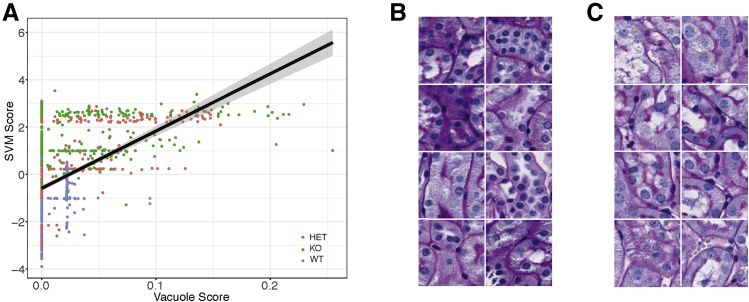
Vacuole score and Support Vector Machine (SVM) in non-glomerular images. A: Correlation of SVM scores from non-glomerular images with vacuole scores determined on the same images, calculated using ImageJ version 1.51h. Black line represents the regression line; gray shading, the 95% CI. B: Montage of examples of wild-type (WT) images with a vacuole score of zero. C: Montage of examples of knockout (KO) images with a vacuole score of zero. Original magnification, ×40 (B and C). HET, heterozygous.

Sodium/Glucose Cotransporter Member 2 (SGLT2) Staining

The kidneys were collected and divided into sections (4 μm thick), as described in the Animals and Samples subsection of Materials and Methods. The slides were processed on the Leica Bond system using an slgt2 antibody (dilution 1:250; 85626; Abcam, Cambridge, UK), 20 minutes of antigen retrieval, and Leica Bond polymer refine detection kit (1298873; Leica Biosystems). Scoring was done by assessing 100 tubuli per animal and scoring each tubule as having a nonconnecting brush boarder or an intact brush boarder. A t-test was performed to determine statistical significance.

Results

DNN analysis was applied to examine if histologic light microscopy image features could be linked with genotype. DNNs were applied to histologic images of kidneys from a previous study in which differences in mesangial matrix expansion were identified (Figure 1).⁹ The study cohort consisted of C57BL/6N males with different alleles for the Far2 gene: i) Far2^{tm2a(KOMP)Wtsi}, hereafter called KO; ii) Far2^B6N, hereafter called WT; and iii) HETs produced by mating the two strains homozygous for both alleles. SVM classifiers were trained using DNN-based QIFs of kidney image patches to make three distinctions: i) between glomerulus and tubule structure, ii) between WT and KO glomeruli, and iii) between WT and KO tubuli.

Glomerular Segmentation

It was first determined if DNNs could perform high-quality glomerular segmentation. The glomerular segmentation SVM model classified pixels within an image as being either inside or outside of a glomerulus (Figure 1). The model was trained on eight example images containing a total of 13 glomeruli that were hand annotated (Figure 1A). Using these training examples, the SVM learned differences in the QIF signatures, distinguishing images whose center pixel is contained within a glomerulus and those whose center pixel is outside of a glomerulus (Figure 1A). The model was then tested on images that were not used for training, including images from animals with different Far2 genotypes than the training examples. The automated pipeline reliably extracted glomerulus locations in images that were not used to train the classifier (Figure 1B). The prediction model is highly accurate, achieving a 92% true-positive rate per pixel at a 10% false-positive rate. Moreover, false-positive pixels cluster around true glomeruli (Figure 1C) rather than being spurious hits in the middle of images. Likewise, false-negative pixels lie just inside the boundary of identified glomeruli (Figure 1C). This model can reliably identify glomeruli, and erroneous predictions are not spurious predictions in tubular tissue, but lie near the boundary of true glomeruli. This allows the model to scan large images of multiple patches to localize glomeruli, which will arise as contiguous blocks of predicted positive pixels (Figure 1D), with few predicted regions not overlapping any glomerulus.

Distinguishing Genotypes Using DNNs

It was next tested whether the DNN features encode measures of kidney histopathology. Aged Far2 KO mice have significantly less MME than WT controls.⁹ Thus, KO and WT mice represent two extremes of glomerular histopathology. An SVM was trained to predict KO versus WT genotype using DNN-based QIFs. For each glomerulus, QIFs were averaged for nine image patches around the center pixel of the glomerulus and an SVM was trained to distinguish WT from KO animals using these averaged glomerular signatures (Figure 3A). The model was trained on 20 example glomeruli (10 from KO animals and 10 from WT animals) and tested on 78 glomeruli from held-out images. The trained model generalized well, achieving an 87% true-positive rate at a 10% false-positive rate (Figure 3B), suggesting that the DNN is sensitive to image features distinguishing the genotypes. In addition to a predicted classification into KO or WT, the SVM classifier reports a score (glomerulus score) quantifying how similar a glomerulus is to the WT versus KO. Large positive scores indicate that a glomerulus is more WT like, and large negative scores indicate that a glomerulus is more KO like. The six glomeruli with the highest scores were from WT animals, and their glomeruli show extensive MME (Figure 3C). Likewise, the six glomeruli with the lowest scores were from KO animals (Figure 3C), and these glomeruli show less MME. Thus, the SVM classification appeared to be specifically sensitive to the MME differences between WT and KO animals. Therefore, glomerulus scores were analyzed for 41 glomeruli from HET animals, which were not used to train the classifier. MMEs were manually scored by eye for these 41 example glomeruli, according to a standard four-point ordinal scale—0 (no damage) through 3 (severe damage).⁹ The DNN-based glomerulus score strongly correlated with the manual MME score (R² = 0.72; P = 9.03 × 10⁻⁸) (Figure 3D), indicating that the model trained to distinguish WT versus KO genotype is implicitly sensitive to MME severity, which it uses to distinguish the genotypes.

Using DNNs for Non-Glomerular Pathology

Because the DNN could distinguish glomeruli from non-glomerular tissue and was sensitive to known histopathology in glomeruli, it was studied whether the DNN could further detect novel pathologic changes in non-glomerular structures. Although MME is well established and widely measured in kidney histopathology, especially in diabetic nephropathy, it is unlikely to be the case that histologic lesions are limited to the glomerulus.¹³ In the original characterization of the Far2 KO renal phenotype, no obvious tubular differences were found on the basis of the manual scoring by a pathologist.⁹ The DNN was applied to image patches outside of glomeruli (ie, images of tubule structures) to test the hypothesis that QIF signatures of non-glomerular structure also differed between the genotypes. An SVM model was trained on 1000 QIF signatures from image patches from KO and WT animals (500 KO, 500 WT), and 21,500 image patches from held-out images of mice from all three different genotypes were tested (Figure 4A). Again, the classifier had strong generalization performance, achieving a 95% true-positive rate at a 10% false-positive rate (Figure 4B), demonstrating that QIFs of non-glomerular structure are sufficient to discern genotype. As with classifying glomeruli as WT or KO, the SVM model reports a confidence score (SVM score) that is significantly different between WT and KO image patches. As with the glomeruli, the HET image patches have an intermediate phenotype, where some HET images classify as WT and others as KO (Figure 4A).

Identification of Differences in Vacuolization and Nuclear Count

To visualize the differences observed by the DNN, montages of 100 representative image patches were generated by selecting the 100 images closest to the mean of the SVM score distributions for KO and WT animals (Figure 4, C and D). These montages show a difference in the number of vacuoles present in the WT proximal tubules compared with the KO tubules. Likewise, montages of the 100 most extreme examples from the KO and WT distributions were generated (Figure 4, E and F), and the difference in vacuoles was confirmed. The extreme examples from WT animals are in the sagittal orientation, whereas the extreme examples from the KO animals are in the transverse orientation. Training and testing data sets for both WT and KO animals contained both sagittal and transverse sections, and the SVM classifier generalized well, demonstrating that it was not confounded by section orientation. Thus, the difference between WT and KO is most easily distinguished in the sagittal plane for the WT and in the transverse plane for the KO. This can be visualized by looking at Figure 4, C and D, which contain representative images for WT and KO animals, respectively. Both montages in Figure 4, C and D, have images in the sagittal and transverse orientation, indicating that the mean SVM score per genotype has examples of each orientation. The separation of sagittal and transverse orientation by genotype only occurs when looking at the extreme examples.

To validate that the SVM classification was sensitive to the presence of vacuoles in non-glomerular tissues, the percentage of non-glomerular tissue covered by vacuoles was quantified using ImageJ. This is referred to as the vacuole score. There is a strong correlation (P < 2.2 × 10⁻¹⁶) between the saturation-based vacuole score and the SVM score (Figure 5A), demonstrating that the SVM score is sensitive to vacuolization.

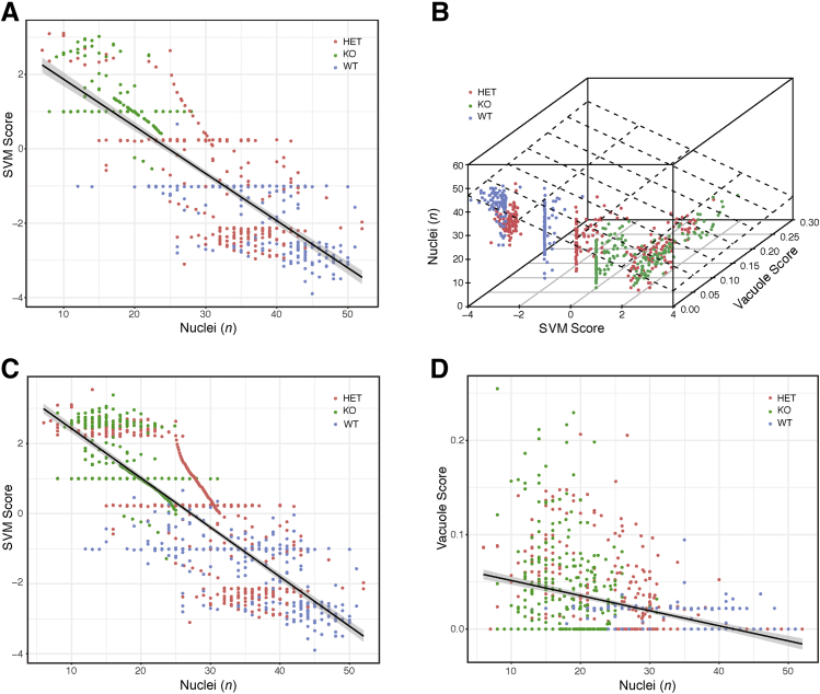
Although the vacuolization result is statistically significant, there was a large range of SVM scores among the image patches that had a vacuole score of zero. When the montages of these images were analyzed, differences in nuclear area and nuclear number were observed (Figure 5, B and C). These differences are quantifiable using standard threshold analysis (GitHub, https://github.com/TheJacksonLaboratory/ImageFeature/tree/master, last accessed March 12, 2019), and they differ between genotypes (Figure 6A). To test whether differences in nuclear count explain differences in the SVM score for images where the vacuole score is not zero, a three-way correlation was performed (Figure 6B) (interactive version available at The Jackson Laboratory, https://www.jax.org/research-and-faculty/resources/histological-phenotyping-and-neural-networks, last accessed March 12, 2019). Figure 6C shows the full cohort of image patches from Figure 5 and that there is a correlation between the SVM score and nuclear count. A combination of vacuole score and nuclear number explains 70% of the variance contained in the SVM score. The nuclear count and vacuole score correlate but not well, and the SVM score is a mixture of both measures (Figure 6D).

Figure 6.

Number of nuclei and Support Vector Machine (SVM) in non-glomerular images. Black line represents the regression line for correlations; gray shading, the 95% CI. A: Correlation between SVM score and number of nuclei for images with a vacuole score of zero. B: Depiction of relationship between vacuole score, nuclear count, and SVM score. An interactive plot is available (The Jackson Laboratory, https://www.jax.org/research-and-faculty/resources/histological-phenotyping-and-neural-networks, last accessed March 28, 2019). C and D: Correlation between SVM (C) and vacuole (D) score and number of nuclei for all non-glomerular images. HET, heterozygous; KO, knockout; WT, wild type.

Relationship between SVM Score and Physiological Measurements

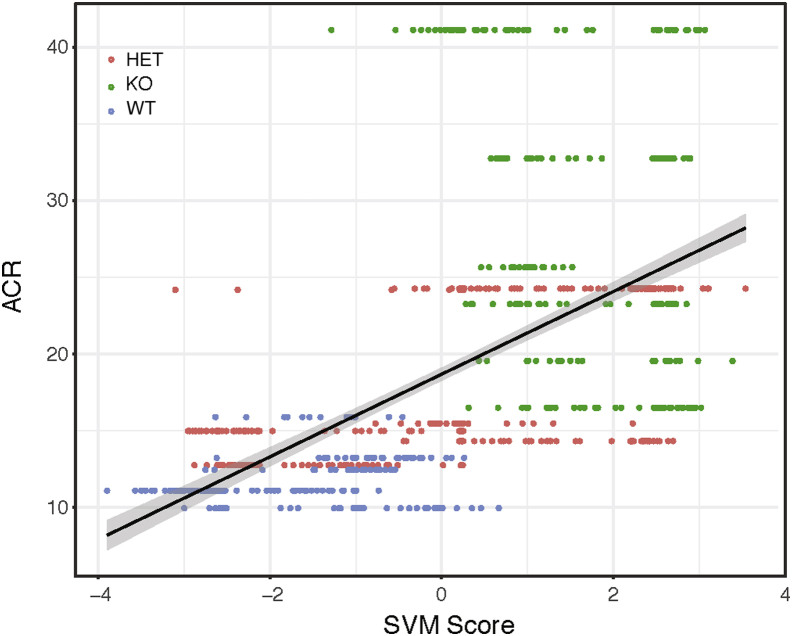
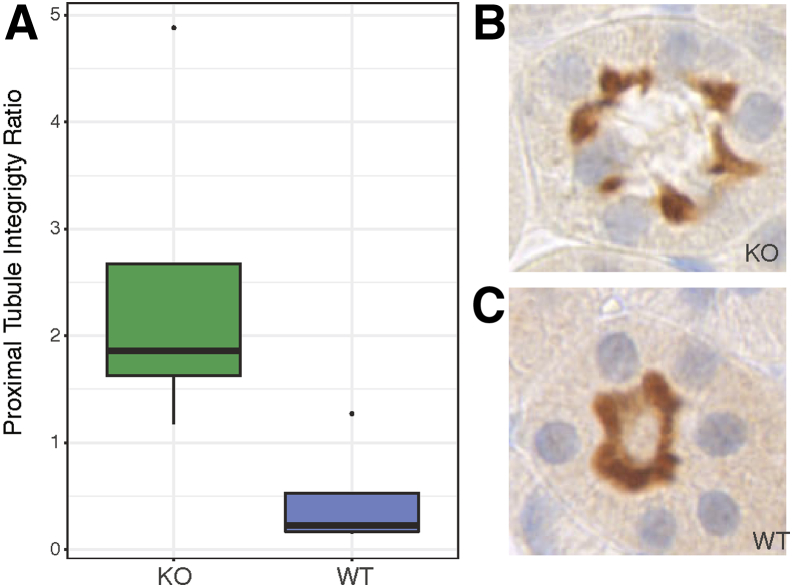
To determine whether the differences in SVM score correlated with renal physiology, non-glomerular SVM scores were studied in relation to glomerular filtration rate data; no relationship was observed. The relationship between non-glomerular SVM scores and urinary albumin/creatinine ratio, however, highlights some interesting findings (Figure 7). There is a threshold of albumin/creatinine ratio/tubular SVM score that separates the KO animals with higher SVM score (>0) and albumin/creatinine ratio (>16 mg/g) from the WT and HET animals. Looking at montages of this separation, a difference was observed in the sharpness of the tubular membranes, with membranes from KO animals having a sharper appearance. This might be due to changes in the integrity of the proximal tubule brush border. Therefore, brush border integrity was studied by staining for SGLT2, and WT animals showed a more intact brush border than KO animals (P = 0.003139) (Figure 8). This clearly links the SVM score from the DNN with a histologic finding relating background genotype to quantifiable differences in the histology and subsequent alterations in physiology. These differences were missed on a labor-intensive traditional scan by trained pathologists (R.E.C.).

Figure 7.

Albumin/creatinine ratio (ACR) and Support Vector Machine (SVM) in non-glomerular image correlation between SVM score and physiological measure of urinary ACR. Black line represents the regression line; gray sharing, the 95% CI.

Figure 8.

SGLT2 staining. A: Quantification of proximal tubule integrity by genotype (P = 0.003139). B: Representative image of a knockout (KO) tubule with loss of SGLT2 positive staining in the lumen of the brush boarder. C: Representative image of a wild-type (WT) tubule stained with SGLT2, depicting an intact brush boarder. Original magnification, ×40 (B and C).

Discussion

There is untapped information in medical images. Much like crime scene investigators on television using information hidden in an image to solve a crime, medical images can be used to explore structure and function beyond traditional clinical and pathologic scores. However, the maximal use of histologic images requires rigorously scoring as much tissue as possible for as many phenotypes as possible. In this study, DNNs were shown to be a significant aid to rigor, throughput, and discovery for histologic analysis. In particular, DNNs were shown to aid in the segmentation and pathologic scoring of kidney tissue and to facilitate the discovery of novel histopathology.

DNNs overcome the time- and labor-intensive rigors of quantitative phenotyping using a reproducible sequence of mathematical transformations without any human-user intervention. The high-dimensional DNN signatures capture thousands of subtle properties of histologic images that can be used to predict other end points, including disease status and physiological outcomes. More important, DNN signatures are unbiased. A significant amount of histologic scoring requires identifying image features of interest and quantifying variation in these features by eye. This process necessarily starts with a researcher's a priori understanding of the relevant histology. In contrast, DNN features were learned by analyzing millions of natural images and learning common patterns.6, 14 The signature of an image across all of these quantitative features encodes histologic features that are not a priori specified, but can be tested for disease relevance. This is analogous to the difference between measuring the expression of a candidate RNA by real-time quantitative PCR and unbiased, genome-wide RNA sequencing. A DNN signature is a holistic readout of a histologic image. As in the genomic revolution, these signatures can be used for both hypothesis testing and hypothesis generation.

In this study, DNN signatures could robustly segment glomeruli from kidney images. Automatic image segmentation is a major field of computer vision research that is currently benefiting greatly from DNN technologies.¹⁵ A pretrained deep neural network is being used to extract features for the downstream machine learning analyses using minimal training data, important for transferring this process to other image problems. These results show that the DNN-based techniques are excellent candidates for general-purpose glomerular segmentation models. The glomerular segmentation pipeline can segment a full-sized mouse kidney section in approximately 40 minutes using 200 cores on the Vermont Advanced Computing Cluster. This makes it possible to analyze more glomeruli than could be accomplished manually. The clustering of incorrect pixel classification around true glomeruli indicates that the boundaries are more difficult for the computer to recognize, but this can be overcome easily when subsequently analyzing the glomeruli themselves. For example, using a box surrounding the detected glomerulus, the genotype classifiers could robustly distinguish genotypes (Figure 3A). Critically, the DNN had few predicted false-positive regions (as opposed to pixels), so post-processing methods are sufficient to address incorrectly classified pixels. At this scale, it is possible to eliminate any technical variation due to subsampling glomeruli from a user-defined region of interest, as effectively all glomeruli in a section can be detected and analyzed. This property makes DNN-based scoring an attractive option for quantitative trait locus mapping and integration into systems biological analysis.

The DNN signatures of both glomeruli and tubule structure were sufficient to classify the Far2 genetic background of the animal. These results demonstrate that DNN signatures encode pathologically relevant features, as these animals are known to differ in both kidney structure and function.⁹ Far2 leads to mesangial matrix expansion through increased production of platelet-activating factor precursors. Increased FAR2 expression in human patients is associated with diabetic nephropathy, lupus nephritis, and IgA nephropathy.⁹ In the case of glomeruli, the DNN signatures specifically encoded MME (Figure 3). The Far2 KO animals are known to have less MME at 12 months of age compared with wild-type controls,⁹ but the traditional scoring system for MME is a subjective ordinal scale.¹² In contrast, the SVM model developed using DNN signatures transformed the categorical distinction between genotypes (WT and KO) into a quantitative glomerular score that strongly correlated with standard MME scores when tested on HET glomeruli. Intuitively, this model asserts that the more similar a HET glomerulus is to a KO glomerulus, the more likely it is to have little MME, and vice versa. An important next step for DNN-based glomerular quantification will be to explicitly model specific glomerular phenotypes as an end point in a multivariate regression using DNN signatures as predictors. Ideally, such a model would be trained using thousands of examples spanning a wide range of models with a spectrum of disease. Our results concerning automatic segmentation and MME demonstrate the feasibility of such efforts.

Machine learning applied to biological image analysis is powerful and advancing rapidly but is often referred to as a black box. This lack of a direct link to definable histology is unsettling to many.¹⁶ The major result of this study is that DNN signatures can distinguish between WT and KO kidney in non-glomerular (mostly tubular) structures. Previous analyses of the tubule structure of these animals by our group and a renal pathologist did not uncover any overt differences.⁹ The DNN signatures, in contrast, robustly distinguished between genotypes (Figure 4). Thus, the DNN is sensitive to subtle patterns that are difficult to pick out from a large set of images but represent true biological differences. However, the DNN signatures have no a priori biological meaning; an image goes in, and a series of numbers comes out. To open the black box and determine the features that the model was using to distinguish the groups, montages of representative and extreme images were used to visualize the subtle distinctions by genotype (Figure 4). This allowed identifying gestalt differences between the groups, including a vacuolization score, number of nuclei, and brush boarder integrity. Renal tubular simplification has been proposed as a response to stress (specifically, hyperglycemia in diabetic conditions).¹³ This difference between WT and KO might be a method of damage control, as MME is delayed in the same mice with the increased tubular damage. The finding that nuclear count correlates with SVM score (Figure 6C) also highlights that the knockout mice have more tubular epithelial cell loss and/or less epithelial proliferation compared with the WT animals. This dovetails nicely with the overall protective mechanisms proposed by the increased vacuoles found in these samples (Figure 5A) and the delayed onset of MME. In addition, with the progression of diabetic nephropathy, tubular membranes can become thick.17, 18 In the KO animals, the DNN has highlighted the presence of tubular simplification, as shown by a lack of SGLT2 staining (Figure 8), which has been shown to occur in diabetic ketoacidosis.¹⁹ In our study, the KO mice lack fatty acyl-CoA reductase 2, a reductase enzyme involved in the conversion of fatty acids to fatty alcohols.²⁰ Albumin reabsorption has been shown to occur in the tubules,²¹ albumin is a normal carrier for free fatty acids, and fatty acid co-uptake in the tubules has already been proposed as a disease mechanism.²² It is possible that the altered lipid profile in the Far2 KO mice causes lipid reabsorption along with albumin, and they increase and accumulate in the tubules. The presence of the vacuoles hampers albumin uptake, resulting in increased urinary albumin. Thus, the tubule alterations observed by the DNN are likely related to functional changes and are consistent with the pathobiology of diabetic nephropathy. All together, these results demonstrate the power of the DNN as an intermediate, hypothesis-generating step that highlights important parts of the image data for deeper analysis (Figure 6B) and points the researcher toward novel mechanistic questions to further explore. Specifically, in this case, non-glomerular changes that make sense in our model were completely missed. The observations were supported by follow-up immunohistochemistry and the enhanced understanding of the role of Far2 in renal function.

The benefits of DNN analysis—rigor, throughput, and discovery—are not limited to kidney histology. These results highlight a paradigm in which histologic images from genetically different strains can be systematically mined for relevant histologic features. The DNN does the grunt work and allows the researcher to hone in on the most relevant features, even those that may have been missed on careful inspection. The DNN is, therefore, a tool to orient us in histologic images and maximize our efforts to those features that are critical for disease processes. As DNN technology steadily improves, more such labor can be moved to machine processing, whereas researcher's effort can be focused on characterizing and validating the most discriminating histologic features.

References

- 1.Matovinović M.S. 1: Pathophysiology and classification of kidney diseases. EJIFCC. 2009;20:2–11. [PMC free article] [PubMed] [Google Scholar]
- 2.Fogo A.B., Kashgarian M. ed 3. Elsevier; Philadelphia, PA: 2016. Vascular diseases. Diagnostic Atlas of Renal Pathology; pp. 295–306. [Google Scholar]
- 3.Johnson R.J., Iida H., Alpers C.E., Majesky M.W., Schwartz S.M., Pritzi P., Gordon K., Gown A.M. Expression of smooth muscle cell phenotype by rat mesangial cells in immune complex nephritis: alpha-smooth muscle actin is a marker of mesangial cell proliferation. J Clin Invest. 1991;87:847–858. doi: 10.1172/JCI115089. [DOI] [PMC free article] [PubMed] [Google Scholar]
- 4.Smolen A.J. Image analytic techniques for quantification of immunohistochemical staining in the nervous system. Quantitative Qual Microsc. 1990;3:208–229. [Google Scholar]
- 5.Janowczyk A., Madabhushi A. Deep learning for digital pathology image analysis: a comprehensive tutorial with selected use cases. J Pathol Inform. 2016;7:29. doi: 10.4103/2153-3539.186902. [DOI] [PMC free article] [PubMed] [Google Scholar]
- 6.Angermueller C., Pärnamaa T., Parts L., Stegle O. Deep learning for computational biology. Mol Systems Biol. 2016;12:878. doi: 10.15252/msb.20156651. [DOI] [PMC free article] [PubMed] [Google Scholar]
- 7.Litjens G., Kooi T., Bejnordi B.E., Setio A.A.A., Ciompi F., Ghafoorian M., van der Laak J.A.W.M., van Ginneken B., Sánchez C.I. A survey on deep learning in medical image analysis. Med Image Anal. 2017;42:60–88. doi: 10.1016/j.media.2017.07.005. [DOI] [PubMed] [Google Scholar]
- 8.Lee J.-G., Jun S., Cho Y.-W., Lee H., Kim G.B., Seo J.B., Kim N. Deep learning in medical imaging: general overview. Korean J Radiol. 2017;18:570–584. doi: 10.3348/kjr.2017.18.4.570. [DOI] [PMC free article] [PubMed] [Google Scholar]
- 9.Backer G., Eddy S., Sheehan S.M., Takemon Y., Reznichenko A., Savage H.S., Kretzler M., Korstanje R. FAR2 is associated with kidney disease in mice and humans. Physiol Genomics. 2018;146:742. doi: 10.1152/physiolgenomics.00118.2017. [DOI] [PMC free article] [PubMed] [Google Scholar]
- 10.Deroulers C., Ameisen D., Badoual M., Gerin C., Granier A., Lartaud M. Analyzing huge pathology images with open source software. Diagn Pathol. 2013;8:92. doi: 10.1186/1746-1596-8-92. [DOI] [PMC free article] [PubMed] [Google Scholar]
- 11.Krizhevsky A., Sutskever I., Hinton G.E. ImageNet classification with deep convolutional neural networks. Commun ACM. 2017;60:84–90. [Google Scholar]
- 12.Sheehan S.M., Korstanje R. Automatic glomerular identification and quantification of histological phenotypes using image analysis and machine learning. Am J Physiol Renal Physiol. 2018;8:296. doi: 10.1152/ajprenal.00629.2017. [DOI] [PMC free article] [PubMed] [Google Scholar]
- 13.Pourghasem M., Shafi H., Babazadeh Z. Histological changes of kidney in diabetic nephropathy. Caspian J Intern Med. 2015;6:120–127. [PMC free article] [PubMed] [Google Scholar]
- 14.Kan A. Machine learning applications in cell image analysis. Immunol Cell Biol. 2017;95:525–530. doi: 10.1038/icb.2017.16. [DOI] [PubMed] [Google Scholar]
- 15.Chilamkurthy S: A 2017 guide to semantic segmentation with deep learning. Available at blog.qure.ai/notes/semantic-segmentation-deep-learning-review (accessed July 19, 2019)
- 16.Ching T., Himmelstein D.S., Beaulieu-Jones B.K., Kalinin A.A., Do B.T., Way G.P. Opportunities and obstacles for deep learning in biology and medicine. J R Soc Interf. 2018;15:20170387. doi: 10.1098/rsif.2017.0387. [DOI] [PMC free article] [PubMed] [Google Scholar]
- 17.Kern W.F., Laszik Z.G., Nadasdy T., Silva F.G., Bane B.L., Pitha J.V. Saunders; Philadelphia, PA: 1999. Atlas of Renal Pathology. [Google Scholar]
- 18.Tyagi I., Agrawal U., Amitabh V., Jain A.K., Saxena S. Thickness of glomerular and tubular basement membranes in preclinical and clinical stages of diabetic nephropathy. Indian J Nephrol. 2008;18:64–69. doi: 10.4103/0971-4065.42336. [DOI] [PMC free article] [PubMed] [Google Scholar]
- 19.Tse R., Garland J., Kesha K., Triggs Y., Yap Z., Stables S. Basal subnuclear vacuolization, Armanni-Ebstein lesions, Wischnewsky lesions, and elevated vitreous glucose and β-hydroxybuyrate. Am J Forensic Med Pathol. 2018;1–3 doi: 10.1097/PAF.0000000000000380. [DOI] [PubMed] [Google Scholar]
- 20.Cheng J.B., Russell D.W. Mammalian wax biosynthesis I: identification of two fatty acyl-coenzyme A reductases with different substrate specificities and tissue distributions. J Biol Chem. 2004;279:37789–37797. doi: 10.1074/jbc.M406225200. [DOI] [PMC free article] [PubMed] [Google Scholar]
- 21.Christov M., Alper S.L. Tubular transport: core curriculum 2010. Am J Kidney Dis. 2010;56:1202–1217. doi: 10.1053/j.ajkd.2010.09.011. [DOI] [PMC free article] [PubMed] [Google Scholar]
- 22.Kees-Folts D., Sadow J.L., Schreiner G.F. Tubular catabolism of albumin is associated with the release of an inflammatory lipid. Kidney Int. 1994;45:1697–1709. doi: 10.1038/ki.1994.222. [DOI] [PubMed] [Google Scholar]