Dejittered Spike-Conditioned Stimulus Waveforms Yield Improved Estimates of Neuronal Feature Selectivity and Spike-Timing Precision of Sensory Interneurons

Abstract

What is the meaning associated with a single action potential in a neural spike train? The answer depends on the way the question is formulated. One general approach toward formulating this question involves estimating the average stimulus waveform preceding spikes in a spike train. Many different algorithms have been used to obtain such estimates, ranging from spike-triggered averaging of stimuli to correlation-based extraction of “stimulus-reconstruction” kernels or spatiotemporal receptive fields. We demonstrate that all of these approaches miscalculate the stimulus feature selectivity of a neuron. Their errors arise from the manner in which the stimulus waveforms are aligned to one another during the calculations. Specifically, the waveform segments are locked to the precise time of spike occurrence, ignoring the intrinsic “jitter” in the stimulus-to-spike latency. We present an algorithm that takes this jitter into account. “Dejittered” estimates of the feature selectivity of a neuron are more accurate (i.e., provide a better estimate of the mean waveform eliciting a spike) and more precise (i.e., have smaller variance around that waveform) than estimates obtained using standard techniques. Moreover, this approach yields an explicit measure of spike-timing precision. We applied this technique to study feature selectivity and spike-timing precision in two types of sensory interneurons in the cricket cercal system. The dejittered estimates of the mean stimulus waveforms preceding spikes were up to three times larger than estimates based on the standard techniques used in previous studies and had power that extended into higher-frequency ranges. Spike timing precision was ∼5 ms.

Introduction

Three questions often addressed in studies of neural coding include the following. What is the optimal stimulus waveform for eliciting a spike in a neuron? What is the nature of the distribution of the waveforms around this “optimal feature” that can elicit a spike? What is the temporal precision with which a spike is linked to the occurrence of a stimulus feature? One general approach toward answering these questions involves presenting a long-duration stimulus waveform capturing the “natural” stimulus regime of the neuron under study, recording the train of spikes elicited by that stimulus, and estimating the average stimulus waveform that precedes each spike (or multiple-spike pattern) in the elicited spike train. Many different algorithms have been used to obtain such estimates, ranging from spike-triggered averaging of stimuli to correlation-based extraction of “stimulus-reconstruction” kernels (Bryant and Segundo, 1976) and spatiotemporal receptive fields (STRFs) (Theunissen et al., 2001). These approaches yield estimates that differ mainly in the manner through which they are normalized and decorrelated from biases in the stimulus set.

As we demonstrate here, these methods all lead to entanglement of the three questions listed above and may result in significant errors with respect to each question. These errors arise from the manner in which the stimulus waveforms are aligned to one another during the averaging or cross-correlation operations. Specifically, these algorithms register the waveform segments to one another based on the precise time of spike occurrence. We know, however, that the biophysical processes underlying sensory transduction, synaptic integration, spike initiation, and synaptic transmission are not perfectly deterministic, and some significant degree of “jitter” in stimulus-to-spike latency is always observable after repeated presentation of identical stimuli (Bryant et al., 1973; Berry et al., 1997; Marsálek et al., 1997; Liu et al., 2001; Zoccolan et al., 2002; Hsu et al., 2004; Uzzell and Chichilnisky, 2004). By ignoring this “intrinsic” jitter, these analytical algorithms all yield distorted estimates of the relevant stimulus waveform and of the variance around that waveform.

We present an algorithm that takes this stimulus-to-spike latency jitter into account and that enables the partial disentanglement of the three questions listed above. The dejittered estimates of the feature selectivity of a neuron provide better estimates of the mean waveform eliciting a spike and have smaller variance around that waveform than estimates obtained using the standard techniques. This procedure disambiguates the uncertainty about the time of occurrence of the stimulus feature from the uncertainty about its waveform and also provides insight into the intrinsic temporal precision with which information from a nerve cell can be decoded.

We applied this technique to study feature selectivity and spike-timing precision of two types of identified sensory interneurons in the cricket cercal system, designated as IN10-3 and IN10-2. The feature selectivity of these cell types was studied in previous experiments using first-order Volterra kernel analysis (Theunissen et al., 1996). Application of the dejittering procedure yields significantly different estimates of the stimulus feature selectivity of these cells. Furthermore, calculations of the lower bound of information encoding rates by these cells, using the “direct method” (Strong et al., 1998) yielded values that were substantially greater than those obtained through the previous kernel-based estimates.

Materials and Methods

Preparation. Experiments were performed on 14 adult female crickets (Acheta domestica) obtained from Bassett's Cricket Ranch (Visalia, CA). Each specimen was selected within 4 h after the final molt and anesthetized on ice for 3-5 min. The legs, ovipositor, and wings were removed, and a window was cut into the dorsal cuticle. Digestive, reproductive, and fat tissues were removed. The abdominal cavity was filled with hypotonic saline solution (O'Shea and Adams, 1981). The preparation was pinned to a plate of silicone elastomer, and a stainless steel platform was inserted beneath the terminal abdominal ganglion and elevated to provide tension on the cercal nerves to facilitate electrode penetration. The mounted preparation was placed within a multidirectional air current stimulator. The stimulator consisted of a central chamber linked to four sets of loudspeakers through enclosed channels (Dimitrov et al., 2003). Movements of the speakers were controlled by power-amplified, computer-generated waveforms, such that the coordinated movement of the speakers generated controlled movements of air across the preparation, thereby stimulating the filiform mechanosensory hairs on the cerci.

Electrophysiology. Neural activity was monitored from the axon of each interneuron in the abdominal nerve cord, near its exit from the terminal abdominal ganglion, using a sharp intracellular microelectrode containing 3 m KCl. Activity was elicited by the presentation of Gaussian noise (GN), air-current stimuli that were band-passed between 5 and 300 Hz and had a root mean square (RMS) speed of 35 mm/s, as calibrated with a low-velocity, air-current sensor (MicroFlown Technologies, Zevenaar, The Netherlands). The stimulus waveforms and neural responses were digitally sampled at 10 kHz (NI PCI-6070E, LabWindows-based proprietary data-logging system; National Instruments, Austin, TX) and stored for subsequent analysis.

Calculation of a dejittered mean stimulus waveform. The algorithm used to dejitter the mean waveform was as follows. First, we collected a set of stimuli, x, from the stimulus-response data set, conditioned on isolated spikes (i.e., spikes that were preceded by a period of ≥30 ms segments devoid of any other spikes and followed by a spike-free interval of ≥30 ms.) Note that this restriction of the analysis to isolated spikes is not essential in general but is done here for the sake of simplicity in illustrating the method. In fact, the procedure could be conditioned on any arbitrary single- or multiple-spike pattern with any arbitrary bounding intervals. Second, we calculated the mean m_x0 of this stimulus set [i.e., the spike-triggered average (STA) for isolated single spikes]. This became our initial model for the mean stimulus waveform preceding a spike. In any association between stimuli and spiking responses of single cells, the STA is equivalent to the stimulus-response correlation. In the case discussed here, m_x0 can be obtained from the STA by normalizing the latter by the response power spectrum, which makes m_x0 equivalent to the first-order Volterra reconstruction kernel (Rieke et al., 1997). Third, we assumed an initial model for the jitter, equivalent to a truncated Gaussian distribution. The core assumption was that the latencies of the recorded spikes had been jittered with respect to the time of the occurrence of the stimulus feature that had elicited those spikes, according to a Gaussian distribution with some variance, σ_t. Note that making this assumption is equivalent to assuming that the temporal resolution of this particular neural response is limited by this variance (i.e., that the time of occurrence of the stimulus feature eliciting a spike would not be resolvable from the spike train of this cell with precision greater than σ_t). For the particular cell under study, the initial value we assumed for this variance (σ_t0) was 3 ms. (As shown below, the technique is robust under a fairly wide range of initial assumed values for the temporal jitter, as long as the value falls within the physiologically realistic range.) We also defined a minimum stimulus-response latency, l_min. In the subsequent realignment procedure, l_min served as a lower bound for shifting the stimuli with respect to the mean. Shifts in time, which were more negative than l_min, were assumed to violate causality in the sense that the spike occurrence time would have occurred before the significant part of the stimulus feature. Fourth, for each individual stimulus waveform sample in the set, we formed all possible time shifts of that waveform in the range l_min to 3σ_t0; for each of the time-shift values for this waveform sample, we calculated the distance between the time-shifted waveform and the mean stimulus waveform calculated in the previous iteration. The distance measure we used was the weighted squared difference between the shifted waveform and the mean waveform, penalized by the weighted square of the shift time (details are presented below). We chose the value of the time shift for this waveform sample that yielded the smallest distance, and we replaced the original waveform sample with this new time-shifted sample. Fifth, after all stimulus waveforms in the set were shifted to minimize their distance from the mean waveform, we calculated a new mean m_x1 of this time-shifted stimulus set. This became the seed value of the mean for the next iteration of dejittering. Sixth, we assessed the temporal variance of the output distribution as the SD of the shift times across the entire data set. This value (σ_ti) became the penalty term for the next iteration of dejittering. Finally, we looped to the fourth step and repeated the subsequent processing steps until the convergence criterion was attained (described in more detail below). The convergence condition results in a minimization of the variance of the dejittered stimulus waveforms around their dejittered mean.

The final mean waveform (m_xf) was assumed to be the best approximation of the dejittered mean waveform preceding a spike, and the distribution of the shift times was likewise taken as our best approximation of the distribution of spike jitter times.

Calculation of shift times from a distance measure. The shift time, t, for a stimulus segment during one iteration of the dejittering procedure was calculated by minimization of a Gaussian distance, d, between that segment and the mean of all segments calculated from the previous iteration as follows:

where x is the residual between the stimulus segment sample and the mean stimulus from the previous iteration, C is the covariance matrix of the stimulus ensemble, σ_t is the assumed variance of the jitter distribution, and t is the specific shift time tested. This distance can be seen as the negative log likelihood of a joint Gaussian model of stimulus and time shifts. Here, for simplicity, we used a diagonal approximation of C, which assumes that individual time samples are independent. This distance, d, was calculated for a range of t values between l_min and +3σ_t at a sampling resolution of 0.1 ms, and the value of t that minimized d was selected as the shift time for that stimulus segment. A shift time was calculated for each different stimulus sample independently, and all segments were realigned according to these relative shift times. The mean of these realigned segments was then calculated and used as the basis for calculating the convergence criterion (see below, Convergence criteria) and, if convergence was not achieved, for calculating the residuals x during the next iteration cycle of the procedure. An additional simplification of the covariance matrix to a multiple of the identity matrix will turn the stimulus distance into a Euclidean distance (sum of squares). Such distance and the iterative re-estimation of features are typically used in standard clustering algorithms, like the k-means (Duda et al., 2000).

Convergence criteria. Convergence of the dejittering procedure was achieved through the minimization of an error function Err_i. The error function corresponded to the percentage change in the square of the residual of the dejittered mean waveforms (see Fig. 4 F) calculated between successive iterations as follows:

Figure 4.

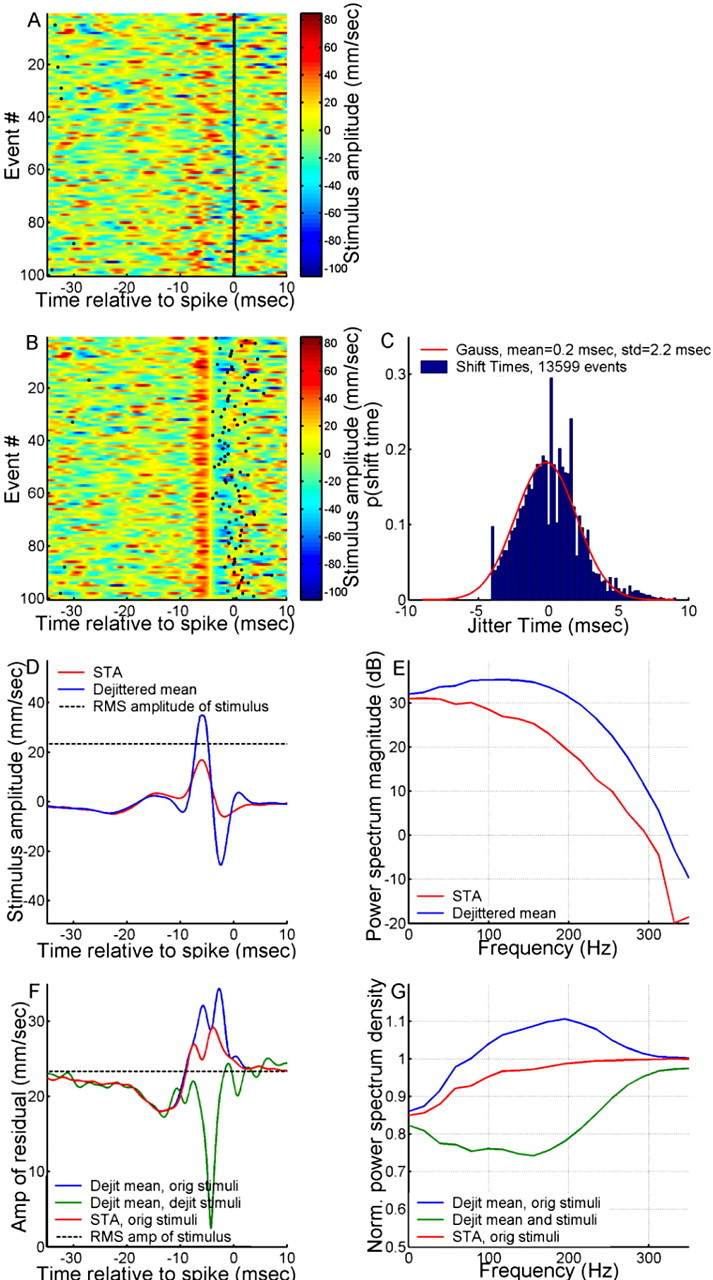
Characteristics of a dejittered mean stimulus. A, Random representative subset of 100 sample segments of stimulus-response data aligned to time of spike occurrence. The vertical black line at t = 0 is the raster plot of spikes superimposed on the color-coded traces of air-current velocity versus time. B, The same random subset of 100 segments of stimulus-response data from A but now dejittered so that their alignment is based on minimal variance of the stimuli. C, Shift times for all 13,600 samples (blue histogram) compared with a Gaussian having an STD of 2.2 ms (red line). D, STA (red trace) and dejittered mean (blue trace). The RMS amplitude of the stimulus is indicated with the dashed black line. E, Power spectra of the STA (red trace) and dejittered mean stimulus (blue trace). F, Red trace, Mean-square residual between the STA and the original (orig) stimulus segments. Blue trace, Mean-square residual between the dejittered (Dejit) mean and the original stimulus segments. Green trace, Mean-square residual between the dejittered mean and the dejittered stimulus segments. The RMS amplitude (amp) of the stimulus is indicated with the dashed black line. G, Power spectra of the residuals, normalized by power spectra of stimulus segments. Colors and abbreviations are the same as in F.

where 〈.〉 denotes the average of the values of the sample waveforms at each time point across all time points, Var(.) denotes the variance vector at each time point across all time points in all samples, stim is the ensemble of dejittered stimulus waveform samples, and i denotes the ith iteration of the dejittering process. Iteration was stopped when Err_i ≤ 10^-6 (i.e., when the relative change between iterations fell to <0.0001%). In general, convergence was achieved in 10-50 iterations.

Calculation of information rates. Estimates of information-encoding rates were calculated from the stimulus-response measurements via two different approaches. The first approach yielded a linear estimate, obtained through the use of stimulus reconstruction techniques (Theunissen et al., 1996; Rieke et al., 1997). The coherence between the air-current stimulus waveform and the spike train response was calculated [Theunissen et al. (1996), their Eq. 8]. Information per frequency was calculated as the negative of the logarithm base 2 of (1 - coherence), and the total information rate was then estimated as the integral of this quantity from 0 Hz up to the highest frequency at which there is significant power in the stimulus [Theunissen et al. (1996), their Eq. 11].

A second estimate of information rate was obtained using the direct method (Strong et al., 1998). Briefly, the unconditional and stimulus-conditioned response probabilities were estimated from data for several different word lengths. Debiased estimates of mutual information rates between the stimuli and associated responses were then obtained using Paninski's “best upper-bound” estimator (Paninski, 2003) for each word length. The best estimate for the information rate was obtained by extrapolating to infinite word length. Note that by using debiased estimates for the information rates, the problem of extrapolation becomes essentially trivial, because rate estimate versus word length becomes essentially a straight line (Kennel et al., 2005).

Results

Illustration of the problem using a thought experiment, formulated as a simulation

Imagine that we are studying a sensory interneuron that is known to operate as a feature detector, that the “optimal stimulus feature” for eliciting a spike has been determined, and that this optimal feature has been presented repeatedly to the cell in the absence of significant background noise (Fig. 1A). We know that the biophysical processes of sensory transduction, synaptic integration, spike initiation, and synaptic transmission at all stages of the nervous system providing input to this interneuron are not perfectly deterministic (Berry et al., 1997; Marsálek et al., 1997; Hsu et al., 2004), and thus we expect that the observed ensemble of stimulus-to-spike latencies in our experiment will have some observable variability around a mean latency. If we create a histogram of spike occurrence times relative to the repeated presentation of a stimulus waveform (Fig. 1B), that distribution will not be a perfect δ function but will have some observable jitter around the mean. Consider the error that will occur in our estimation of the stimulus waveform that we presented, if we calculate an STA of the stimulus waveforms preceding the spikes. The procedure starts with the alignment of all instances of the presented waveforms relative to the time of occurrence of the spike elicited by each waveform (Fig. 1C). The observed distribution of spike times in Figure 1B is translated into a jittering of the actual presented waveforms with respect to one another in C. The subsequent averaging of the waveforms with this imposed jitter (Fig. 1C, bold trace) yields an estimated stimulus waveform that is distorted with respect to the true waveform. Figure 1D shows a comparison of this jittered mean (solid black trace) with the original waveform (solid gray trace). This distortion is equivalent to a blurring of the true waveform with a point-spread function identical to the actual spike train jitter distribution, similar to the manner in which an image is blurred by the point-spread function of an optical system. We note that calculation of a Volterra or Wiener stimulus-reconstruction kernel (Bryant and Segundo, 1976; Rieke et al., 1997), an STRF (Theunissen et al., 2001), or any other method based on the cross-correlation between each spike in the ensemble and the stimulus waveforms preceding those spikes would also result in such a blurring of the estimated waveform.

Figure 1.

A thought experiment to define the jitter problem using simulated recordings. A, Top trace, A segment of simulated stimulus consisting of three identical optimal features presented at random intervals, with no background noise. Bottom trace, Three spikes elicited by those stimulus features. B, Superposition of 500 examples of the stimulus waveform at an expanded timescale, with a raster plot of the jittered occurrence times of spike selicited by those 500 repetitions, and a histogram of those times immediately below. C, A total of 24 randomly selected samples of the stimulus wave form of the total data set of 500. These stimulus segments have been shifted with respect to one another to bring all of their elicited spikes into alignment (i.e., the vertical line to the lower right of the set of waveforms is the realigned spike raster). The mean of all realigned waveforms (i.e., the STA) is shown with the solid line. D, Comparison of the STA from C (solid line) with the actual stimulus waveform from B (gray line) and the dejittered mean (dotted trace).

A much-improved estimate of the true mean stimulus waveform can be obtained by taking the spike-timing jitter into account. This dejittering is achieved by shifting the ensemble of sample waveforms with respect to one another in a manner that minimizes the variance around the subsequent mean while penalizing large shifts (see Materials and Methods). The application of this procedure to the simulated data in Figure 1C yielded the dotted black trace in Figure 1D, which is a much better estimate of the actual waveform (solid gray trace) than the STA (solid black trace).

We note that it is possible, in principle, to use an approach to dejittering that is the inverse of the approach presented here (i.e., to shift spike train segments that code for the stimulus features in a manner that maximizes the correlation between those spike train segments). This would require different measures of closeness, specific to the response space of the neuron, such as the metric space approach developed by Victor and Purpura (1996).

Time scale of the stimulus-to-spike latency jitter in a sensory interneuron

We applied this algorithm to study the stimulus-response properties of two pairs of mirror-symmetric primary sensory interneurons in the cercal sensory system of the cricket Acheta domestica. This mechanosensory system mediates the detection and analysis of low-velocity air currents and can be thought of as a low-frequency, near-field extension of the animal's auditory system (Palka et al., 1977; Bacon and Murphey, 1984; Kämper and Kleindienst, 1990; Miller et al., 1991; Theunissen et al., 1996). The interneurons receive direct excitatory synaptic input from filiform mechanosensory hairs on the animal's two antenna-like cerci at the rear of the abdomen. The sensory stimuli we used to drive the interneurons were dynamic air currents with velocity waveforms characterized by GN, band-passed between 5 and 300 Hz. Figure 2 shows one typical segment from an experiment in which a 10 s stimulus was repeated 100 times. Figure 2A3 shows a 500 ms segment of this GN stimulus waveform, and A1 shows the corresponding raster plot of the spike trains elicited by the 100 repeated presentations of that waveform segment. Figure 2A2 is the histogram of these spike-occurrence times (peristimulus time histogram). This segment of data demonstrates the wide range of stimulus-to-spike latency distributions that are typically elicited by GN stimuli. The three panels in Figure 2B show the central 60 ms segment of the data shown in Figure 2A at an expanded time scale, which captures the sharpest distribution of spike times from that segment.

Figure 2.

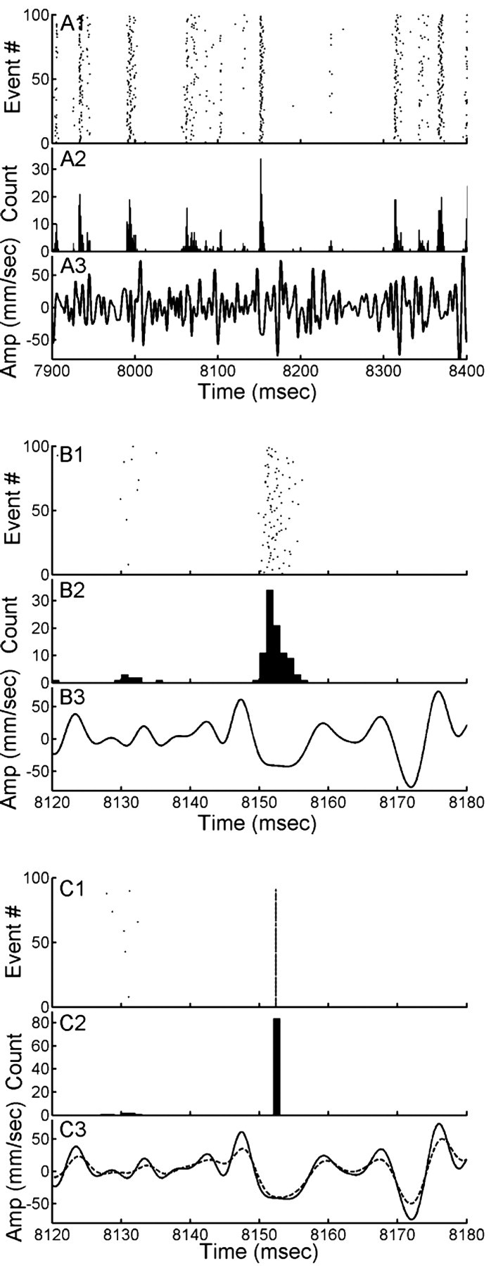
An experiment to illustrate the jitter problem, using a mechanosensory interneuron. A1, Raster of the spike times elicited by 100 repetitions of this waveform. A2, Histogram of this raster plot using 1 ms time bins. A3, A 0.5 s segment of the Gaussian noise stimulus waveform. B, The central 60 ms segment of the data shown in A at an expanded time scale. C1, Spike-time raster plot after realignment of the spikes in the distribution shown in B. C3, Dashed line, Mean of all stimulus segments realigned to the evoked spikes (i.e., the STA). C3, Solid line, The actual stimulus waveform (as in B). Amp, Amplitude.

Figure 2C illustrates the result of calculating the STA of the stimulus waveform segments from the subset of data shown in Figure 2B. Figure 2C1 is the raster plot of spikes after their realignment into precise registration. Figure 2C2 is the histogram of these spikes (i.e., all fall into a single bin), and the dashed trace in C3 is the average of all 100 stimulus segments after their realignment (i.e., the STA for these spikes). For comparison, the solid line in that bottom panel is the actual stimulus waveform that had been presented repeatedly to the animal (and was therefore the real mean waveform leading up to any spikes). It is clear that the STA yields a distorted image of the true waveform.

Dejittering a sample of spike-conditioned stimulus waveforms

Although the thought experiment (Fig. 1) and the demonstration of spike jitter (Fig. 2) were based on repeated presentations of identical stimulus waveforms for the sake of illustration, the dejittering protocol we introduce below does not require such repeated stimulus presentations nor does it require a priori knowledge about the optimal stimulus. Rather, we used a single nonrepeating, long-duration, band-passed, Gaussian noise waveform. Figure 3A shows a 500 ms segment of the air current stimulus waveform. The corresponding spike train response (containing five spikes) elicited by this segment is shown directly above the stimulus trace. The times of spike occurrence are indicated on the stimulus waveform (Fig. 3A) with small colored circles. Figure 3B shows the superposition of the stimulus waveform segments preceding all five spikes, aligned with respect to the times of spike occurrence (defined as t = 0; note that Fig. 3B-D are at an expanded time scale). The bold, dashed red curve is the STA of all stimulus segments. Figure 3C shows the results of shifting this set of stimulus segments with respect to one another to recover an estimate of the stimulus waveform that minimizes the distortion caused by spike-timing jitter. The extent to which each of the five waveforms was shifted in time is indicated by the small colored circles. The mean of the set of shifted waveforms is shown as the bold blue curve. Figure 3D compares the preshifted STA from B with the dejittered mean from C. The dejittered mean clearly has larger amplitude than the standard STA, with the frequency composition of the increased component biased toward the higher-frequency range of the waveform.

Figure 3.

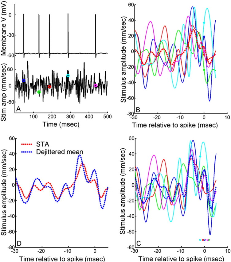
Illustration of the dejittering algorithm. A, A 500 ms segment of stimulus (bottom trace) and corresponding intracellular membrane potential with five spikes elicited by that stimulus (top trace). The time of spike occurrences are marked on the stimulus waveform with colored circles. Stim amp, Stimulus amplitude. B, Five 35 ms segments of the stimulus waveforms preceding each of the five spikes in A, locked to the times of spike occurrence at t = 0 ms. The color of each stimulus waveform matches the colored markers in A. The mean (i.e., spike-triggered average) waveform is shown with the dashed red line. C, The same five 35 ms segments, as shown in B, but now dejittered. The time-shifted spike times are shown by the markers under the waveforms. The mean is shown with the dashed blue line. D, Comparison of dejittered mean (blue dashed trace) with STA (red dashed trace) for the data.

The results of a complete analysis of this IN10-3 stimulus-response dataset are shown in Figure 4. All instances of isolated single spikes (preceded and followed by spike-free intervals of ≥30 ms) were extracted from a 33 min recording, yielding a sample size of ∼13,600 stimulus segments. Figure 4A shows raster plots of a random representative subset of 100 of the sample segments of stimulus-response data. Each horizontal raster line is color coded to indicate the stimulus velocity versus time, with colors toward red indicating positive velocity and colors toward blue representing negative velocity. The black dot at time 0 indicates the time of occurrence of the spike elicited by the waveform within that particular sample. All of the stimulus waveforms in Figure 4A are locked in their alignment to the spike occurrence times. Figure 4B shows the result of dejittering these waveforms, assuming a value of 3 ms for σ_t0 during the procedure. The redistribution of the stimulus-response raster lines resulting from this dejittering procedure results in a visibly sharpened registration of the stimulus waveforms across the raster set and a visibly scattered deregistration of the spike occurrence times. The distribution of shift times to achieve the optimal dejittered mean had a σ_t value of 2.2 ms (Fig. 4C). Figure 4D compares the uncorrected spike-conditioned mean (i.e., the STA; red trace) with the dejittered mean (blue trace) across all 13,600 samples in the dataset. The dejittered mean stimulus had a peak amplitude 2.6 times higher than that of the STA. The dejittered mean also had a greater relative proportion of its power extending into the higher-frequency range than did the STA, as can be seen from a comparison of the power spectral densities of the STA and dejittered mean waveforms (Fig. 4E). Note that, as discussed previously, the STA is equivalent to the first-order Volterra kernel calculated with the same data in this particular case, because the correlation time of the mean was less than the interspike interval.

Functional significance of the dejittered mean waveforms

The dejittered mean waveform is visibly different from the STA. However, it is somewhat problematic to assess the functional significance of this difference. It is not meaningful, for instance, to simply perform a stimulus reconstruction using the different types of waveforms (e.g., dejittered mean and STA or Volterra kernel), calculate the mean-squared error between the estimated and actual stimulus in all cases, and compare the results. The STA (equivalent to the Volterra kernel for this case) will always give a lower mean-squared error than a dejittered mean, because the Volterra kernel is derived precisely to minimize the mean-squared error (without taking the jitter into account). The animal could not, of course, take the jitter into account (i.e., it could not perform the dejitter operation a priori), because it can't recover the precise times at which the dejittered estimates occurred before the spike. Within this context, the jitter σ_t can be interpreted as the degree of uncertainty about the timing of the feature that elicited the spike (i.e., the limiting temporal resolution of the cell).

The experimentor can, however, perform an informative calculation that takes jitter into account and illustrates how the use of dejittered mean stimuli can help to disambiguate the uncertainty about the time of occurrence of a stimulus feature from the uncertainty about its waveform. The red trace in Figure 4F is the SD between the stimulus and the STA at each time sample in the experimental ensemble, with the STA and sample both aligned to the time of spike occurrence. This residual reflects the combination of all factors that contribute to error in the estimation, including temporal jitter of the spikes, coarseness in the tuning of the cell to a distribution of suboptimal waveforms around the optimal mean waveform, any correlation structure in the stimulus set, and all other biological factors that contribute to “noisiness” in the neural processing stream. The corresponding red trace in Figure 4G is the power spectrum of that residual, normalized by the power spectrum of the stimulus. This shows the fraction of the power in the signal that is not explained by the STA and is analogous to the mean-squared error of a reconstruction (Roddey et al., 2000).

In contrast, the green traces in Figure 4, F and G, were calculated using the dejittered mean waveform and dejittered stimulus segments. That is, before subtracting the dejittered mean waveform from each stimulus segment sample in the test ensemble, that stimulus segment was time shifted to the alignment with respect to the dejittered mean that had been determined to yield the minimal residual for that specific segment. This procedure specifically excluded the contribution of the temporal uncertainty to the residual error, leaving only the uncertainty about the stimulus waveform. The gap between the red and green traces in both panels corresponds to the error introduced by the STA (or Volterra kernel) in estimating the waveform of the mean stimulus: the higher the red trace above the green, the greater is the relative error of the STA compared with that of the dejittered mean. It is clear that the dejittered mean yields a much lower residual error than the STA over the most significant segment of the stimulus waveform preceding the spikes. The spike jitter contributed a significant amount of residual error to the STA-based estimate of the stimulus waveform, and this error is biased toward the high-frequency end of the sensitivity range of the cell.

Note that the red and green traces in Figure 4F are equivalent to the SDs across all of the spike-locked and dejittered stimulus traces, respectively. Consideration of these different estimates of variance leads to substantially different interpretations of the feature selectivity and stimulus-response dynamics of the cell. The variance across all of the dejittered stimulus signals around the dejittered mean waveform (green trace) is lower than the signal RMS throughout the entire duration of the segment shown here, with the lowest point (i.e., the greatest significance) associated with the period between 3 and 5 ms before the spike. The residual decreases to nearly 0 at ∼4 ms before the spike, indicating an extremely high degree of significance near this time point in the stimulus waveform (i.e., a very high degree of stimulus waveform selectivity).

Consideration of the variance around the STA (Fig. 4F, red trace) is problematic: within the critical time segment leading up to the spike, the variance across all stimulus signals around the STA residual actually climbs to a maximum value that is larger than the RMS signal amplitude itself, and would indicate that the shape of the STA has no significance during that period. Interpretation of that red curve would lead to the conclusion that the significant part of the waveform was the segment between 10 and 20 ms preceding the spike, in which the amplitude of the STA is negligible. Thus, interpretation of the feature selectivity and stimulus-to-spike latency on the basis of an STA is problematic. Here, again, a conventional Volterra kernel or STRF would also yield the same problematic results.

The blue traces in Figure 4, F and G, were calculated by subtracting the dejittered mean waveform directly from each of the stimulus segments, locked to the spike time rather than shifting the dejittered mean to the position yielding the smallest residual. (This is equivalent to performing a stimulus reconstruction using the dejittered mean instead of the Volterra kernel.) As expected, the residual and its power spectrum are both greater (i.e., worse) than those obtained with the STA. This is a corollary to the fact that the STA was constructed to give the minimum least-squared fit to the unshifted set of stimulus segments; although the dejittered kernel is a more accurate and precise estimate of the actual mean waveform that elicited each spike, it results in a poorer estimate of the stimulus if the jitter is not taken into account.

Sensitivity of the technique to the value of σ_t0 used for the calculations

In general, the dejittering procedure is robust over a broad range of values for the assumed spike jitter penalty term σ_t0, as long as that value is kept within a physiologically reasonable range. Figure 5A is a surface plot comparing the dejittered mean waveforms obtained from several independent dejittering procedures, run on the same data set, using different values for σ_t0 (y-axis). The STA corresponds to the first horizontal color band at the top of the plot (σ_t0 = 0). Each successive color band below that first one was calculated with σ_t0 increased by 0.2 ms. Calculations initiated with all values of σ_t0 converged to essentially identical estimates. Figure 5B is a surface plot of the distributions of shift times for each value of the penalty term σ_t0. Each horizontal color band represents the output distribution of shift times for a different value of the penalty term. The probability of a specific shift time is shown by color, with blue colors indicating a low probability of that shift time and red colors indicating a high probability. The curve in Figure 5C shows SDs of the final shift distributions (σ_tf). The SDs stop increasing for values of σ_t0 greater than ∼4 ms, demonstrating that the dejittered mean is insensitive to variation of the penalty term beyond that value.

Figure 5.

Dependence of the dejittered mean shape and σ_tf on σ_t0. A, Mean output stimulus for each value of input penalty term σ_t0. The top row (σ_t0 = 0) shows the original STA. B, Probability distributions of the output shift times at 1 ms resolution for each value of the penalty term σ_t0. The top row (σ_t0 = 0) shows the spike times before dejittering. The color scale has been truncated from a maximum value of p (shift time) = 1 at σ_t0 = 0, shift time = 0. C, STD of dejitter shift times (σ_tf) for each value of input penalty term σ_t0.

Interanimal variability of the dejittered mean stimuli and σ_t for this type of interneuron

The data presented in the preceding sections were recorded from a single identified interneuron designated as a left IN10-3 [the 10-3 interneurons exist as mirror-symmetric pairs in the terminal abdominal ganglion, with one right (R) IN10-3 and one left (L) IN10-3]. To assess the interanimal and interpair variability in the dynamic response characteristics of this cell type, we repeated the experimental analysis and extracted dejittered mean stimuli for a sample of seven R IN10-3s and seven L IN10-3s from different animals. The results are shown in Figure 6. The uncorrected STAs are shown in Figure 6A, and the dejittered means are shown in Figure 6B. The dejittered means were very similar to one another in duration, amplitude, and waveform. Each dejittered mean was significantly larger in amplitude than its corresponding uncorrected STA by a factor ranging from 2 to 3. Figure 6C shows the jitter distributions for these seven cells on an expanded time scale. The mean σ_t for this sample of seven IN10-3 cells was 2.08 ± 0.26 ms.

Figure 6.

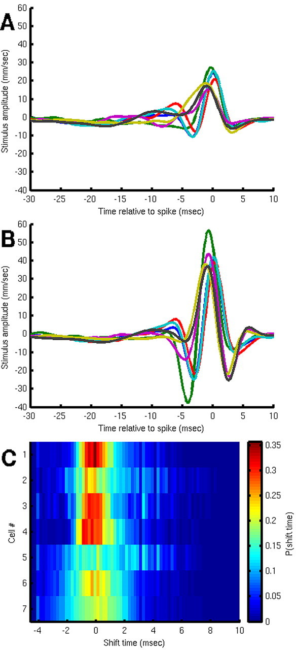
Composite average stimulus waveforms for a sample of seven cells from class 10-3. A, Standard STAs. B, Dejittered means. C, Histograms of the shift times for the seven IN10-3 cells at an expanded time scale, with color coding for the fraction of samples shifted by the indicated time.

Every terminal abdominal ganglion in each cricket also contains another mirror-symmetric pair of interneurons designated as right and left IN10-2 (Jacobs and Murphey, 1987). The four 10-3 and 10-2 INs comprise a functionally discrete subunit of the cercal system: they have the lowest stimulus threshold of all of the cercal interneurons and are the only cells that encode information about the direction of air-current stimuli in the horizontal plane in this low-stimulus velocity range (Miller et al., 1991). Their directional sensitivities are mutually orthogonal: each has a selectivity for stimuli primarily originating from within one quadrant, and their peak directional selectivities are distributed at 90° intervals around the horizontal plane. Previous studies using Volterra analysis suggested that the 10-2 and 10-3 cells have indistinguishable dynamical sensitivities (Theunissen et al., 1996). To assess the dynamic response characteristics of IN10-2, we repeated the experimental analysis and extracted dejittered mean stimuli for a sample of seven R and L IN10-2s from different animals. The results are shown in Figure 7. The uncorrected STAs are shown in Figure 7A, and the dejittered means are shown in Figure 7B. The dejittered means were very similar to one another in duration, amplitude, and waveform. Each dejittered mean was significantly larger in amplitude than its corresponding uncorrected STA by a factor ranging from 2 to 2.5. Figure 7C shows the jitter distributions for these seven cells on an expanded time scale. The mean σ_t for this sample of seven IN10-2 cells was 2.33 ± 0.12 ms.

Figure 7.

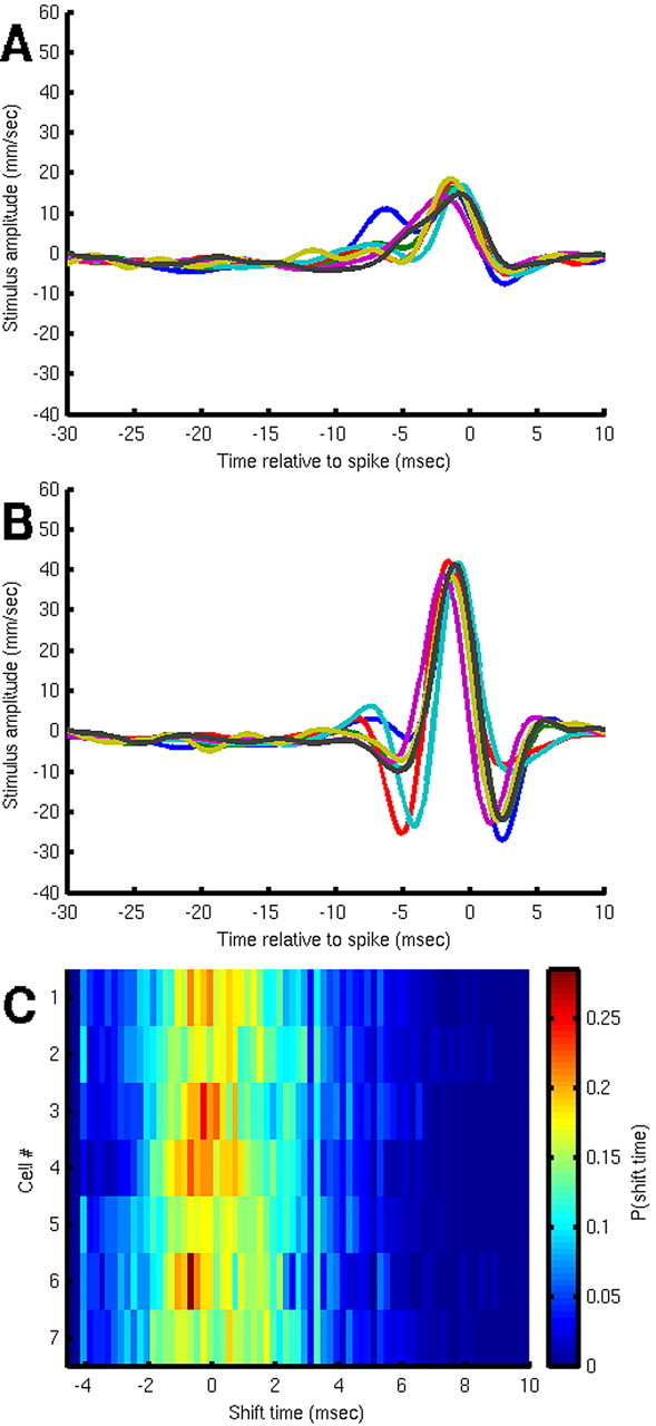
Composite average stimulus waveforms for a sample of seven cells from class 10-2. A, Standard STAs. B, Dejittered means. C, Histograms of the shift times for the seven IN10-2 cells at an expanded time scale, with color coding for the fraction of samples shifted by the indicated time.

Figure 8 shows a comparison of the composite averages of the dejittered mean stimulus waveforms for the IN10-3 (solid black trace) and IN10-2 (dashed gray trace) sample sets. There is no significant difference between the two composite means, nor was there a significant difference between the two values for σ_t. This indicates that all four cells have functionally equivalent dynamic stimulus-response selectivities and characteristics within the stimulus regime tested here.

Figure 8.

Comparison of the composite average dejittered mean stimulus waveforms for seven examples of each of the cell classes 10-3 (solid black curve) and 10-2 (dashed gray curve). Error bars on each curve represent 1 SD across the corresponding sample.

Calculation of the information rate for IN10-3 using a direct method

In previous studies, the information-encoding rates for a sample of 10-2 and 10-3 interneurons were calculated on the basis of a Volterra kernel-based analysis (Theunissen et al., 1996). Considering the extent to which the Volterra kernels were shown above to misrepresent the stimulus selectivities of these cells, we recalculated the encoding rate for an IN10-3 using a method that was independent of assumptions about stimulus selectivity (Buracas et al., 1998; Borst and Theunissen, 1999). This was done using a version of the direct method (Strong et al., 1998; Paninski, 2003). The calculation was based on stimulus-response data from the same IN10-3 preparation used for Figures 2, 3, 4, 5, within a regime in which the mean spike rate was 10.8 spikes/s. The information rate for this cell was calculated to be 27.2 ± 0.4 bits/s using the direct method. In contrast, the kernel-based calculation identical to that used in our previous studies, applied to the same data, yielded a rate of 20.3 ± 1.5 bits/s. This represents an upward revision of the calculated encoding rate by a factor of 1.34.

Discussion

Jitter happens. Although spike jitter has been characterized and considered in many studies (Bryant et al., 1973; Mainen and Sejnowski, 1995; Victor and Purpura, 1996; Berry et al., 1997; Marsálek et al., 1997; Reich et al., 1997; Reinagel and Reid, 2000; Keat et al., 2001; Liu et al., 2001; Zoccolan et al., 2002; Hsu et al., 2004; Uzzell and Chichilnisky, 2004), it is not taken into account fully when analyzing feature selectivity with standard analysis techniques. Conventional methods for the derivation of the STA, STRF, or Volterra and Wiener kernels misrepresent the class of stimulus waveforms that elicit spikes in a cell: those techniques underestimate the amplitude and bandwidth of the mean stimulus waveform and overestimate the variance of the waveforms around that mean. Application of this dejittering algorithm to cercal sensory interneurons 10-2 and 10-3 yielded estimates of the mean waveforms preceding isolated spikes that were up to three times larger in amplitude than the STAs extracted from the same data sets and also had greater relative power extending into a higher-frequency range. In addition, the dejittered estimates of the feature selectivity of IN10-3 were more accurate and more precise than estimates obtained using the STA: the variance of the dejittered stimuli around the mean stimulus was substantially lower than the variance around the STA.

Conventional techniques also obscure the statistical structure of the stimulus-response latency relationship. Dejittered estimates disambiguate the uncertainty about the time of occurrence of the stimulus feature from the uncertainty about its waveform. In addition, and perhaps more important, the variance σ_t of the jitter distribution provides an explicit metric for assessing the temporal precision with which a spike is linked to the occurrence of a specific stimulus feature. An implicit assumption is that the sensory system knows its own feature selectivity as well as its intrinsic temporal uncertainty and does not need such tools to obtain that information. The output of the cell provides information about the stimulus waveform and its time of occurrence, but that information has some irreducible degree of uncertainty.

It is important to emphasize that dejittering cannot violate the data processing inequality. Information rates cannot be “improved” by dejittering; rather, the model of stimulus selectivity is improved, enabling a better estimation of stimulus-response properties than other similar models that do not take explicit account of uncertainties in spike timing and/or feature waveform.

Implications for the assessment of temporal precision

A consideration of the magnitude of σ_t is informative with respect to assessments of the time scale for neural coding. Many analyses of neural coding require an explicit determination (or assumption) of the intrinsic or natural time scale with which the spike train of a cell must be decoded. The width of the jitter distribution provides a rough estimate for the lower bound on that precision, assuming a linear encoding scheme (Theunissen and Miller, 1995). Regardless of the precision with which an upstream decoder could resolve the time of occurrence of a postsynaptic potential from one of the interneurons we studied, the time of occurrence of the stimulus event that triggered the corresponding spike in that interneuron could not be resolved in time with more precision than the jitter distribution we observed. In the cells studied here, the temporal uncertainty of the occurrence time for isolated spikes (calculated as ±2 σ_t of the jitter distribution) was ∼5 ms, which was ∼20% of the duration of the significant portion of the dejittered waveform. This jitter in the stimulus-to-spike latency therefore appears to impose a significant constraint on the temporal accuracy of any linear decoding operation that could be performed on the spike train from this cell. However, that overall system-level temporal precision could be improved beyond this limit at a subsequent stage, through ensemble processing of the spike train of this cell along with spike trains from additional cells carrying redundant and/or complimentary information (Chichilnisky and Kalmar, 2003).

Note that information about other independent stimulus features cannot, in principle, be extracted from the distribution of spike latencies, even if latencies correlate with such features. This is because the absolute latencies are not available to later stages of the nervous system. However, additional information about feature identity is potentially obtainable from relative latencies in population responses. In this case, the response of a single cell should not be considered in isolation but as part of a multicell response pattern.

Factors contributing to stimulus-to-spike timing jitter

Although the dejittered mean yields a more accurate estimate of the feature and frequency selectivity of a cell, this approach still cannot completely disambiguate the different intrinsic and extrinsic factors that contribute to the observed spike-timing variance. The GN waveforms we used for our determination of the dejittered means and σ_t values contained a broad range of stimulus waveforms. As shown in Figure 2, some waveform segments elicited spikes with relatively high-timing precision (i.e., low-jitter σ_t). Such segments are very similar to the dejittered mean waveforms, and we might surmise that these are near-optimal stimuli. However, the long-duration GN stimuli also contained many more segments that were significantly different from the dejittered mean waveform but were still similar enough that they elicited spikes. The inclusion of the responses from these suboptimal stimulus segments in the dejittering procedure would be expected to increase the value calculated for σ_t relative to the value that would be derived for spikes elicited by near-optimal stimuli. This is because the net blurring function can be conceptualized as a convolution of the “minimal jitter” distribution (e.g., resulting from presentation of a truly optimal stimulus, attributable to all lumped factors contributing to biophysical noise) with the distribution emerging from the responsiveness of the cell to a range of stimuli around the mean. Although the shape of the dejittered mean will not necessarily be effected by the inclusion of these less-than-optimal stimulus-response samples (i.e., if their deviation from the mean waveform is symmetric), the estimated σ_t will depend on the specific dataset used for the calculation and will always overestimate the minimal jitter resulting from biophysical noise alone.

Implications for kernel-based analyses of information-encoding rates

To the extent that the time scale of spike jitter is significant with respect to the correlation time of the mean waveform and to the extent that the dejittered mean differs in shape from a kernel, we lose confidence in the relevance of the stimulus-reconstruction approach and the measure of “gain” as a means for characterizing information-coding rates. The use of a distorted kernel to generate an estimate of the stimulus waveform leads to a severely low-passed underestimate of that stimulus. The subsequent use of this distorted stimulus estimate to derive a lower bound to the encoding rate results in a bound that is lower than we had imagined, to a degree that is difficult to quantify. To borrow a term from the realm of political science, we misunderestimate the true coding rate (for discussion, see Hsu et al., 2004).

There are alternate approaches for estimating encoding rates that make no explicit assumptions about details of stimulus representation, such as the direct method (Strong et al., 1998; Paninski, 2003). Although these methods provide no explicit information about the feature selectivity of a cell, they can provide accurate estimates of the total information available to potential downstream decoders that are insensitive to spike jitter. Our application of the direct method to stimulus-response data from IN10-3 yielded an estimate for the information encoding rate that was a factor of 1.3 higher than the rate estimated using the conventional kernel-based stimulus reconstruction method we used in previous studies. Thus, even in the case of this IN10-3, which appears to be well approximated as having a nearly linear encoding scheme, calculation of the lower bound on information-encoding rate by integration under the gain curve led to a substantial underestimate of its channel capacity.

Reappraisal of encoding by this four-cell group of cricket cercal interneurons

Beyond this upward revision of the estimate of the coding capacity by IN10-3, the results of this analysis also led us to a refinement of our understanding of the feature sensitivity of this set of interneurons. These four interneurons appear to have much higher feature selectivity than was realized previously, and the mean stimulus waveform eliciting a spike differs significantly from kernel-based estimates with respect to amplitude and frequency composition. Previous estimates indicated a stimulus-frequency selectivity limited to the range between 5 and 80 Hz, with peak sensitivity at 15 Hz (Theunissen et al., 1996). The new estimates, based on the dejittered means, indicate that stimulus frequency selectivity extends to ≥200 Hz, with peak sensitivity ranging between 100 and 150 Hz.

This range brackets the wing-beat frequencies of predatory wasps (Gnatzy and Heusslein, 1986) and other signals of neuro-ethological significance that had been considered previously as undetectable by these cells. One possible role for this group of low-threshold, directionally selective cells is as an “early warning” system for detecting the approach and direction of such flying predators.

References

- Bacon JP, Murphey RK (1984) Receptive fields of cricket (Acheta domesticus) are determined by their dendritic structure. J Physiol (Lond) 352: 601-613. [DOI] [PMC free article] [PubMed] [Google Scholar]
- Berry MJ, Warland DK, Meister M (1997) The structure and precision of retinal spike trains. Proc Natl Acad Sci USA 94: 5411-5416. [DOI] [PMC free article] [PubMed] [Google Scholar]
- Borst A, Theunissen FE (1999) Information theory and neural coding. Nat Neurosci 2: 947-957. [DOI] [PubMed] [Google Scholar]
- Bryant HL, Segundo JP (1976) Spike initiation by transmembrane current: a white-noise analysis. J Physiol (Lond) 260: 279-314. [DOI] [PMC free article] [PubMed] [Google Scholar]
- Bryant HL, Marcos AR, Segundo JP (1973) Correlations of neuronal spike discharges produced by monosynaptic connections and by common inputs. J Neurophysiol 36: 205-225. [DOI] [PubMed] [Google Scholar]
- Buracas GT, Zador AM, DeWeese MR, Albright TD (1998) Efficient discrimination of temporal patterns by motion-sensitive neurons in primate visual cortex. Neuron 20: 959-969. [DOI] [PubMed] [Google Scholar]
- Chichilnisky EJ, Kalmar R (2003) Temporal resolution of ensemble visual motion signals in primate retina. J Neurosci 23: 6681-6689. [DOI] [PMC free article] [PubMed] [Google Scholar]
- Dimitrov AG, Miller JP, Gedeon T, Aldworth Z, Parker AE (2003) Analysis of neural coding using quantization with an information-based distortion measure. Network 14: 151-176. [PubMed] [Google Scholar]
- Duda RO, Hart PE, Stork DG (2000) Pattern classification, Chap 10, Ed 2. New York: Wiley.
- Gnatzy W, Heusslein R (1986) Digger wasp against crickets. I. Receptors involved in the antipredator strategies of the prey. Naturwissenschaften 73: 212-215. [Google Scholar]
- Hsu A, Borst A, Theunissen FE (2004) Quantifying variability in neural responses and its application for the validation of model predictions. Network 15: 91-109. [PubMed] [Google Scholar]
- Jacobs GA, Murphey RK (1987) Segmental origins of the cricket giant interneuron system. J Comp Neurol 265: 145-157. [DOI] [PubMed] [Google Scholar]
- Kämper G, Kleindienst H-U (1990) Oscillation of cricket sensory hairs in a low-frequency sound field. J Comp Physiol [A] 167: 193-200. [Google Scholar]
- Keat J, Reinagel P, Reid RC, Meister M (2001) Predicting every spike: a model for the responses of visual neurons. Neuron 30: 803-817. [DOI] [PubMed] [Google Scholar]
- Kennel M, Shlens J, Abarbanel HDI, Chichilnisky EJ (2005) Estimating entropy rates with Bayesian confidence intervals. Neural Comp, in press. [DOI] [PubMed]
- Liu RC, Tzonev S, Rebrik S, Miller KD (2001) Variability and information in a neural code of the cat lateral geniculate nucleus. J Neurophysiol 86: 2789-2806. [DOI] [PubMed] [Google Scholar]
- Mainen ZF, Sejnowski TJ (1995) Reliability of spike timing in neocortical neurons. Science 268: 1503-1506. [DOI] [PubMed] [Google Scholar]
- Marsálek P, Koch C, Maunsell J (1997) On the relationship between synaptic input and spike output jitter in individual neurons. Proc Natl Acad Sci USA 94: 735-740. [DOI] [PMC free article] [PubMed] [Google Scholar]
- Miller JP, Theunissen FE, Jacobs GA (1991) Representation of sensory information in the cricket cercal sensory system. I. Response properties of the primary interneurons. J Neurophysiol 66: 1680-1689. [DOI] [PubMed] [Google Scholar]
- O'Shea M, Adams ME (1981) Pentapetide (proctolin) associated with an identified neuron. Science 213: 576-569. [DOI] [PubMed] [Google Scholar]
- Palka J, Levine R, Schubiger M (1977) The cercus-to-giant interneuron system of crickets. I. Some aspects of the sensory cells. J Comp Physiol 119: 267-283. [Google Scholar]
- Paninski L (2003) Estimation of entropy and mutual information. Neural Comput 15: 1191-1253. [Google Scholar]
- Reich DS, Victor JD, Knight BW, Ozaki T, Kaplan E (1997) Response variability and timing precision of neuronal spike trains in vivo. J Neurophysiol 77: 2836-2841. [DOI] [PubMed] [Google Scholar]
- Reinagel P, Reid RC (2000) Temporal coding of visual information in the thalamus. J Neurosci 20: 5392-5400. [DOI] [PMC free article] [PubMed] [Google Scholar]
- Rieke F, Warland D, de Ruyter van Steveninck R, Bialek W (1997) Spikes: exploring the neural code, Chap 2. Boston: MIT.
- Roddey JC, Girish B, Miller JP (2000) Assessing the performance of neural encoding models in the presence of noise. J Comput Neurosci 8: 95-112. [DOI] [PubMed] [Google Scholar]
- Strong SP, Koberle R, de Ruyter van Steveninck RR, Bialek W (1998) Entropy and information in neural spike trains. Phys Rev Lett 80: 197-200. [Google Scholar]
- Theunissen F, Miller JP (1995) Temporal encoding in nervous systems: a rigorous definition. J Comput Neurosci 2: 149-162. [DOI] [PubMed] [Google Scholar]
- Theunissen FE, Roddey JC, Stufflebeam S, Clague H, Miller JP (1996) Information theoretical analysis of dynamical encoding by four identified primary sensory interneurons in the cricket cercal system. J Neurophysiol 75: 1345-1364. [DOI] [PubMed] [Google Scholar]
- Theunissen FE, David SV, Singh NC, Hsu A, Vinje WE, Gallant JL (2001) Estimating spatio-temporal receptive fields of auditory and visual neurons from their responses to natural stimuli. Network 12: 289-316. [PubMed] [Google Scholar]
- Uzzell VJ, Chichilnisky EJ (2004) Precision of spike trains in primate retinal ganglion cells. J Neurophysiol 92: 780-789. [DOI] [PubMed] [Google Scholar]
- Victor JD, Purpura KP (1996) Nature and precision of temporal coding in visual cortex: a metric-space analysis. J Neurophysiol 76: 1310-1326. [DOI] [PubMed] [Google Scholar]
- Zoccolan D, Pinato G, Torre V (2002) Highly variable spike trains underlie reproducible sensorimotor responses in the medicinal leech. J Neurosci 22: 10790-10800. [DOI] [PMC free article] [PubMed] [Google Scholar]