Limited Segregation of Different Types of Sound Localization Information among Classes of Units in the Inferior Colliculus

Abstract

The auditory system uses three cues to decode sound location: interaural time differences (ITDs), interaural level differences (ILDs), and spectral notches (SNs). Initial processing of these cues is done in separate brainstem nuclei, with ITDs in the medial superior olive, ILDs in the lateral superior olive, and SNs in the dorsal cochlear nucleus. This work addresses the nature of the convergence of localization information in the central nucleus of the inferior colliculus (ICC). Ramachandran et al. (1999) argued that ICC neurons of types V, I, and O, respectively, receive their predominant inputs from ITD-, ILD-, and SN-sensitive brainstem nuclei, suggesting that these ICC response types should be differentially sensitive to localization cues. Here, single-unit responses to simultaneous manipulation of pairs of localization cues were recorded, and the mutual information between discharge rate and individual cues was quantified. Although rate responses to cue variation were generally consistent with those expected from the hypothesized anatomical connections, the differences in information were not as large as expected. Type I units provide the most information, especially about SNs in the physiologically useful range. Type I and O units provide information about ILDs, even at low frequencies at which actual ILDs are very small. ITD information is provided by a subset of all low-frequency neurons. Type V neurons provide information mainly about ITDs and the average binaural intensity. These results are the first to quantify the relative representation of cues in terms of information and suggest a variety of degrees of cue integration in the ICC.

Introduction

A natural hypothesis is that parallel pathways of the brainstem auditory system have arisen to process different aspects of acoustic information. This hypothesis seems to hold true at lower stages in the auditory pathway, especially for the processing of sound localization cues. The medial superior olive (MSO) extracts interaural time difference (ITD) information from low-frequency sounds and is relatively insensitive to interaural level differences (ILDs) (Goldberg and Brown, 1969; Yin and Chan, 1990). Conversely, lateral superior olivary units are dominated by ILD cues (Boudreau and Tsuchitani, 1968; Guinan et al., 1972a,b; Tollin and Yin, 2002). Meanwhile, units in the dorsal cochlear nucleus (DCN) have been implicated in the processing of monaural spectral cues through both behavioral (Sutherland et al., 1998; May, 2000) and physiological (Young et al., 1992; Imig et al., 2000; Reiss and Young, 2005) studies.

Projections from these nuclei (along with others) form partially overlapping maps within the central nucleus of the inferior colliculus (ICC), presumably producing regional variations of connections (Roth et al., 1978; Adams, 1979; Brunso-Bechtold et al., 1981; Oliver et al., 1997). The nature of the convergence of sound localization information within the ICC is an important outstanding question.

Work by Ramachandran et al. (1999) provides some hypotheses about ascending projections to ICC neurons. They describe three classes of neurons in the ICC of decerebrate cats exhibiting sustained responses to tone bursts (see Fig. 1). Type V units (see Fig. 1A) are found only in the low-frequency region of the nucleus, are binaurally excited (EE), and are sensitive to ITDs (Ramachandran and May, 2002). Because the physiology of these neurons mimics that of MSO neurons (Yin and Chan, 1990), it is hypothesized that the MSO is their dominant source of input. Type I units (see Fig. 1B) are found in all frequency regions; they are excited by contralateral tones and inhibited by ipsilateral tones (EI). Because they are sensitive to ILD cues (Davis et al., 1999), the lateral superior olive (LSO) is hypothesized to be their dominant input. Finally, type O cells (see Fig. 1C) are found in all frequency regions and have complex binaural response maps (Davis et al., 1999), the contralateral portion of which resembles that of a DCN type IV unit. Evidence from blocking the dorsal acoustic stria suggests that their dominant input arises from the DCN (Davis, 2002).

Figure 1.

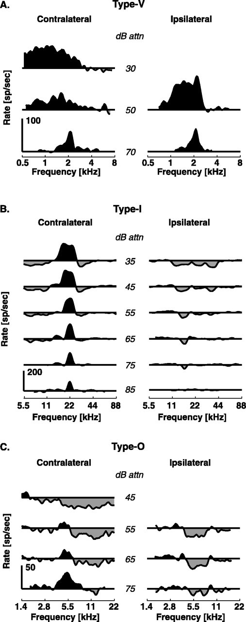
Response maps typical of the classes of ICC units exhibiting sustained responses to tones. Driven rates are calculated over a 200 ms tone duration, and spontaneous rates are subtracted to reveal inhibition. At 0 dB attenuation (attn), the sound level is ∼100 dB sound pressure level. A, Type V unit, characterized by EE responses and little to no inhibition. B, Type I unit, characterized by EI responses and sideband inhibition. C, Type O unit, characterized by an island of excitation at low levels of contralateral stimulation turning to inhibition at higher levels. Responses to ipsilateral tones are typically inhibitory.

The hypothesized segregation of inputs from the various sources described above suggests a partial segregation of different classes of sound localization information in the ICC. Using information theoretical techniques, this work addresses how information about spatial localization cues is represented among the physiological classes of ICC neurons. Emphasis is placed on the convergence of information about different cue types (ITD, ILD, and spectral cues) under the assumption of a rate code. The representation is examined under conditions in which two different cues are manipulated simultaneously, to examine the effects of cue interaction. Although there are differences among the physiological types defined by Ramachandran et al. (1999), it is clear that considerable integration of different classes of localization cues occurs at the level of the ICC.

Materials and Methods

Surgical procedure. Experiments were performed on adult cats with clean external ears and middle ears free from infection. At the beginning of surgery, cats were given atropine sulfate (0.1 mg, i.m.) to reduce mucous secretions and dexamethasone (2.0 mg, i.m.) to reduce edema. A surgical plane of anesthesia was achieved with xylazine (1 mg/kg, i.m.) and ketamine (40 mg/kg, i.m.) and maintained with supplemental doses (∼15 mg/kg ketamine, i.v.) as needed. The cat was decerebrated by opening a hole through the parietal bone and aspirating the brain between the superior colliculus and the thalamus, completely severing the thalamus and cortex from the brain stem. Once the decerebration was complete, anesthesia was discontinued. The cephalic vein was cannulated to allow the intravenous perfusion of drugs and fluids during the course of the experiment. A tracheotomy was performed to facilitate breathing. The cat's temperature was maintained between 37.5 and 38.5°C with a feedback-controlled heating pad.

The IC was exposed dorsally by drilling through the skull overlying the occipital cortex and aspirating cortex until the IC was visible. In most cases, the bony part of the overlying tentorium was removed to gain full access to the IC. The ear canals were exposed and fitted with ear tubes for sound delivery, and the bullae on both sides were vented with ∼30 cm of PE 90 tubing to prevent pressure buildup in the middle ear. At the end of the experiment, the cat was killed with an overdose of barbiturate anesthetic. All procedures were performed in accordance with the guidelines of the Institutional Animal Care and Use Committee of the Johns Hopkins University.

Recording procedure. Recordings were made in a sound-attenuating chamber. Sounds were presented via speakers placed on the free end of the hollow ear bars. The acoustical system was calibrated in situ for both ears with a probe tube microphone placed ∼2 mm from the cat's tympanic membranes. This system produces a fairly uniform response between 40 Hz and 35 kHz [see Rice et al. (1995) for typical examples of the calibration]. Platinum/iridium microelectrodes were used for single-unit recording. Single units were isolated with a Schmitt trigger or a template-matching program (Alpha-Omega Engineering, Nazareth, Israel). All data are based on clear single-unit recordings.

Electrodes were advanced dorsoventrally through the IC to sample units with various best frequencies (BFs). Electrode entry into the central nucleus was determined by physiological cues as follows. As the electrode was advanced, BFs first decreased, then increased. This frequency reversal occurred ∼1-2 mm below the surface and signified transition from the dorsal cortex or external nucleus into the central nucleus (Rose et al., 1963; Merzenich and Reid, 1974; Aitkin et al., 1975). Neurons in the dorsal cortex or external nucleus were often tuned poorly, adapted rapidly, or exhibited marked offset responses; neurons within the ICC were usually sharply tuned with short latencies (Merzenich and Reid, 1974; Aitkin et al., 1975). The ventral edge of the ICC was reached when the BF jumped abruptly from high frequencies (∼30-40 kHz) to low frequencies (<1 kHz), signifying entry into the dorsal nucleus of the lateral lemniscus (Aitkin et al., 1970), or when background activity to auditory stimulation disappeared.

The BFs of isolated single units were determined manually, and characterization stimuli were presented to compare the unit to known response types of ICC neurons, as in Figure 1. All characterization stimuli were 200 ms in length including 10 ms linear rise/fall edges, followed by an 800 ms silent interval. The average discharge rate over the entire 200 ms interval was used for the classification; Ramachandran et al. (1999) used the last 150 ms of the stimulus for their rate calculations; the response classifications are robust and do not change if rates are computed from 150 or 200 ms. If rates are computed over shorter intervals (say the first 50 ms), inhibitory regions become harder to see, so classification becomes more difficult. Spontaneous rates were calculated over the last 400 ms of the silent period.

Classification was done as follows. Units that were excited by monaural tones presented to either ear and that had little inhibition in the response map were classified as type V. Units that had responses to contralateral BF tones that were excitatory at low levels but turned to inhibition at high sound levels were classified as type O. Units that were excited at all contralateral BF tone levels and displayed clear sideband inhibition were classified as type I. The majority of these units were also inhibited by ipsilaterally presented tones, although there were three high BF units classified as type I that were binaurally excited with clear sideband inhibition. Consistent with Ramachandran et al. (1999), no type V neurons were found with BFs >4.8 kHz. The classification of very low BF (<1 kHz) neurons is difficult; almost all of the low-BF neurons in our sample had type V characteristics.

Once the unit was characterized as type V, I, or O, analysis stimuli (described below) were presented for the remainder of the recording time. The stimulus level was chosen to be near the center of the dynamic range of the unit under study.

Stimulus design. Three sets of virtual space stimuli were constructed. Each stimulus set consisted of a 330 ms broadband frozen noise token (sampled at 100 kHz; interstimulus interval, 1 s) that was manipulated to vary independently over two parameters. Each parameter was adjusted in five steps, for a total of 25 stimuli per set. These 25 stimuli were presented in fixed order, and the individual stimuli were interleaved; that is, all 25 stimuli were presented once, then the entire stimulus set was repeated, etc.

The first stimulus set, shown in Figure 2 A, was designed to probe the differential sensitivity to ITD and ILD cues. The noise token was filtered through a spatially averaged head-related transfer function (HRTF); the HRTFs used here were obtained from the cat data of Rice et al. (1992). Filtering the noise token through a spatially averaged HRTF imparts to the stimulus the spectral characteristics of the head and ear canal, independent of spatial location. The stimulus was then split into two streams (one for each ear) that were delayed relative to one another to impart an ITD. Five ITDs were used, at -160, -80, 0, 80, and 160 μs, in which a positive value indicates the contralateral stimulus is leading. Physiological ITD-azimuth functions vary with frequency, elevation, and head size and depend on whether transient or steady-state values are measured (Kuhn, 1977; Roth et al., 1980). The values chosen here correspond approximately to spatial locations in the horizontal plane of -60, -30, 0, 30, and 60° azimuth, on a hard sphere with the approximate diameter of a cat's head; transient measurements for clicks yield somewhat longer delays for the same azimuths (Roth et al., 1980). Finally, the two streams were attenuated relative to one another to impart an ILD. Five ILDs were used, at -13.8, -8.4, 0, 8.4, and 13.8 dB. When averaging the ILDs measured from cat HRTF functions over frequency and elevation, these values also correspond approximately to -60, -30, 0, 30, and 60° azimuth. The two most popular methods of imposing ILDs in the literature are the contra-constant method, in which the contralateral level is held fixed while the ILD is manipulated with the level in the ipsilateral ear (Rose et al., 1966; Geisler et al., 1969; Davis et al., 1999; Park et al., 2004), and the average binaural intensity (ABI) constant method, in which the average summed level is held constant and the levels in both ears are adjusted to create the ILD (Phillips and Irvine, 1981; Wise and Irvine, 1985; Semple and Kitzes, 1987). In the first two stimulus sets, a variation of these methods was used. For the five ILDs, the levels in the ipsilateral ear were set to 0, 0, 0, -8.4, and -13.8 dB (regarding the reference level), and the levels in the contralateral ear were set to -13.8, -8.4, 0, 0, and 0 dB. This nonstandard method of ILD adjustment was originally done so that, in a plot of response rate versus ILD, the effects of ILD could be dissociated from the effects of monaural response to either contralateral or ipsilateral stimulation, something that cannot be done with either the contra-constant or the ABI constant method. The third stimulus set (described below) was designed to disambiguate binaural and monaural responses more directly.

Figure 2.

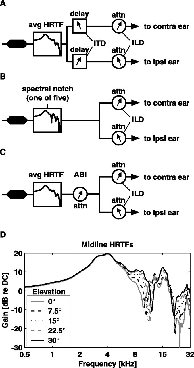
Stimulus construction. A, ITD/ILD stimulus set. Frozen noise was filtered through a cat HRTF, averaged over spatial location to give the location-independent spectral characteristics of the pinnae and ear canal. The noise was then copied into two streams, on which an ITD and an ILD were placed. B, SN/ILD stimulus set. The frozen noise was filtered through one of five HRTFs showing a prominent SN, split into two streams and attenuated relative to one another. C, ABI/ILD stimulus set. As in A, the frozen noise was filtered through the spatially averaged HRTF. It was then attenuated to one of five levels before being split into two streams that are attenuated relative to one another. The ILD was imposed such that the ABI was preserved. D, The five HRTFs used in the SN/ILD stimulus set. All were taken from the midline, at 0° azimuth. Note the prominent first SN, which shifts to higher frequencies as the elevation is increased. The SN/ILD stimulus set was resampled before presentation such that the notch for 15° elevation fell on the BF. avg, Average; attn, attenuation; contra, contralateral; ipsi, ipsilateral; DC, zero frequency.

The second stimulus set was designed to probe the differential sensitivity to ILD and spectral notch (SN) cues (Fig. 2 B). The SN cue was imparted by filtering the frozen noise token through one of five HRTFs containing a prominent SN. These HRTFs, shown in Figure 2 D, were taken from the azimuth midline and correspond to 0, 7.5, 15, 22.5, and 30° elevations. The stimulus was then split into two streams, and an ILD cue was imparted as in the ITD/ILD stimulus set. Note that, because the stream splitting occurs after filtering, the same spectral shape is sent to each ear. Interaural spectral differences are not considered in this study. Before presentation, the stimuli in this set were resampled to place the SN of the 15° stimulus at the BF of the unit under study. Although this resampling sometimes drew the SNs outside of the physiological range (6-20 kHz) (Musicant et al., 1990; Rice et al., 1992), these stimuli are useful in probing general spectral encoding properties of the neurons.

The third stimulus set (Fig. 2C) was designed to probe the segregation of ABI and ILD cues and disambiguate monaural level responses from true binaural sensitivity. In this set, the frozen noise was again filtered through the spatially averaged HRTF. The ABI of the resultant stimulus was adjusted to range in five steps from -8 to +8 dB, referenced to the average system attenuation. This stimulus was then split into two streams that were attenuated relative to one another in such a manner as to preserve the ABI. For this set, ILDs of -16, -8, 0, 8, and 16 dB were used.

Information analysis. The mutual information (MI) between the response of a neuron, R, and an individual localization cue, X, is defined as follows (Cover and Thomas, 1991):

(1)

Similarly, the MI between R and both localization cues X and Y is as follows:

(2)

For notational convenience, the MI between the response and both localization cues will be referred to as MI_FULL, and the MI between the response and a single cue X will be referred to as MI_X.

In this analysis, the response of the neuron was defined as the spike count during stimulus presentation. The window for counting spikes began at stimulus onset and extended 20 ms past stimulus offset, to fully capture any stimulus-dependent effects.

The probability distribution of the stimulus parameters, p(x,y), is uniform at 1/25, because there are 25 stimuli in every set presented an equal number of times. The number of stimuli sets the maximum value of MI_FULL at log₂(25) = 4.64 bits. Similarly, the maximum value of MI_X (or MI_Y)islog₂(5) = 2.32 bits, because there are five equally likely values for X or Y. The joint probability function p(x,y,r) was estimated as the number of times spike count r was observed while the stimulus with parameters (x,y) was presented, divided by the total number of stimulus presentations.

The relationship of MI_FULL to MI_X and MI_Y is important in understanding how individual neurons can represent multiple cues. A full derivation, provided in the appendix, yields the following:

(3)

Equation 3 shows that the mutual information between the response and the full stimulus set is not necessarily equal to the sum of the information about the individual cues. The difference, MI(X;Y|R), is known as the confounded information (introduced by Reich et al., 2001). A non-zero value of the confounded information occurs when the spike count in response to parameter X changes depending on the value of Y. Although the stimulus parameters X and Y were originally independent of one another, conditioning on the spike count can induce mutual information between them. From a coding point of view, the information a neuron provides about X can be increased by independent knowledge of Y, although the stimuli are formally independent a priori.

Because MI cannot be negative, small or noisy samples are subject to estimation bias (Treves and Panzeri, 1995). The sample size bias was estimated by a bootstrap procedure as the difference between the mean of 500 bootstrap estimations of MI and the measured MI (Efron and Tibshirani, 1998). The bootstrap data sets for each stimulus were computed by randomly selecting, with replacement, N spike counts from the set of recorded spike counts for that stimulus, where N is the number of stimulus repetitions. Because of the high number of stimulus repetitions typically achieved (median, 70 repetitions), the estimated bias for MI_FULL was quite low (median, 0.1 bits or 8.3% of the median value of raw MI). Simulations using homogeneous Poisson processes reveal that this debiasing technique leaves a residual bias that declines with the number of stimulus repetitions. The debiased MI estimates converge to within 20% of the true value at ∼20 stimulus repetitions. Other debiasing techniques (Panzeri and Treves, 1996; Strong et al., 1998) give almost identical results. In this study, a small number of units (10) were included from which between 10 and 20 stimulus repetitions were collected; these units do not influence the reported data trends. All values of MI presented in this report are debiased.

The monaural index. For analysis of ABI versus ILD encoding, the monaural index was used. This index compares the fraction of variance in the rate response accounted for by the contralateral sound level (fv_c) to the fraction of variance accounted for by the ipsilateral sound level (fv_i). If r_i,(j,k) is the ith response to the stimulus with the contralateral level equal to j and the ipsilateral level equal to k, then fv_c is calculated as follows:

(4)

Here, μ represents the mean rate response to all stimuli with the ipsilateral level equal to 0, regardless of contralateral level, and μ_j represents the mean to all stimuli with the contralateral level equal to j and the ipsilateral level equal to 0. There are five such stimuli in the ABI/ILD set, with levels (16,0), (8,0), (0,0), (-8,0), and (-16,0), where the values in parentheses are the contralateral and ipsilateral levels, respectively. fv_i is calculated in a similar manner, but from a different set of stimuli with the contralateral level held constant at 0 and the ipsilateral level allowed to vary. With these values, the monaural index is as follows:

(5)

When the monaural index is equal to 1, none of the variance in the rate is accounted for by the ipsilateral level; the unit is monaural to the contralateral ear. Similarly, when the monaural index is equal to -1, the unit is monaural to the ipsilateral ear. When the monaural index is 0, the rate variance accounted for by the contralateral level exactly matches that accounted for by the ipsilateral level (i.e., the neuron is fully binaural). Note that a binaural unit can be sensitive to ABI or to ILD, and in either case, the monaural index will go to zero.

Results

At least 10 repetitions of one or more stimulus sets were collected from 124 units in 31 cats. A total of 105 of these units were successfully classified according to the scheme of Ramachandran et al. (1999), including 32 type O cells, 46 type I cells, and 27 type V cells. The remaining units represent 11 onset units, 3 units with ambiguous BFs and 8 units with unclassifiable response maps, and are not considered in this study.

Responses to the SN/ILD and ITD/ILD stimulus sets

Figure 3 presents two examples of the relationship between spatial cue information and spike count. The top row shows data for a 6 kHz type I unit investigated with the SN/ILD stimulus set. The spike rate is plotted as a function of the two stimulus parameters in Figure 3A. For this example, MI_FULL is 1.75 bits. The contours on the back walls show the mean and SD of the spike rate when considering only the response to the individual cues, achieved by collapsing the surface along one axis (i.e., averaging across the other cue). Figure 3, B and C, replots these spike rate contours as a function of the ILD and SN, respectively. This neuron is much more sensitive to changes in the ILD than in the SN, because MI_ILD is 1.29 bits, whereas MI_SN is only 0.21 bits. As indicated by Equation 3, MI_FULL does not equal the sum of the MIs carried about the individual localization cues. The bottom row presents SN/ILD data collected from another type I unit with a similar BF (5.1 kHz). This unit is more sensitive to changes in the SN than to changes in the ILD.

Figure 3.

Extracting the MI to the full stimulus set and to the individual location cues. A, The surface shows the mean response rate as a function of the ILD and SN (surface-smoothed with cubic spline interpolation). Contours on the vertical walls of the plot show the mean (±1 SD) of the rate as a function of ILD or SN only. The debiased MI is given above the plot with the bias estimate in parentheses. B, Mean rate versus ILD. C, Mean rate versus SN. D-F, Same for another unit showing more SN sensitivity. sp, Spikes.

To show that there are consistent differences among the responses dependent on unit type, examples of the normalized discharge rate profiles to the localization cues are plotted in Figure 4. For every stimulus set, each neuron produced five rate profiles in response to each parameter. Because these five rate profiles often changed as a function of the second parameter, all five are included in this analysis. Rate profiles are normalized to their maximum discharge rate for comparison across units. Because in many cases there are too many data to see details in the plots, only the 40 rate profiles with the largest single-cue MIs are shown. Profiles corresponding to MI_X < 0.1 bits are not included to eliminate insensitive units.

Figure 4.

Rate profiles of responses to the SN/ILD and ITD/ILD stimulus sets. Each profile has been normalized to its maximum response. Thin gray lines represent individual rate profiles, and thick black lines represent the means of all rate profiles in each category. oct, Octave.

Fig. 4 (left column) shows the rate profiles of the three unit types in response to the ILD. Type I units (Fig. 4, middle row) have the most consistent responses to the ILD stimuli, with almost all of the rate profiles showing a peak when the contralateral stimulus is louder, corresponding to sound sources in the contralateral hemifield. Type V units (Fig. 4, top row) usually show a peak at midline, at which the overall binaural level is highest for these stimulus sets. Type O units (Fig. 4, bottom row) show the most diversity in their responses, with both contralateral and ipsilateral selectivity. These results are in agreement with those described by Davis et al. (1999).

Fig. 4 (middle column) shows the rate profiles of the three unit types in response to SN manipulations, plotted as a function of the center frequency of the SN in octaves referenced to the BF. Type I units show a trough-shaped response centered on the BF, in which the notch is centered directly over the excitatory area of the unit. This profile is consistent with the type I response map (Fig. 1B) in that the response is weakest when the SN is centered directly over the excitatory portion of the response map and strengthens as the SN moves away from the BF. This occurs although the frequency range spanned by the SNs is narrow and does not usually extend beyond the excitatory area of the type I units.

The type V rate profiles show little modulation by the SN. This is possibly because of their wide excitatory bandwidths, which are not obviously truncated by inhibition. The type O units again show the most diversity in their rate profiles. In particular, there are a few peak-like responses to the SN, some monotonically increasing responses, and a number of trough-like responses.

Fig. 4 (right column) shows the rate profiles in response to ITD manipulations. The ITD responses are quite variable across all unit types, although this diversity is most marked in the type O population. Indeed, of all the unit types, the type O units seem to exhibit the most rate modulation in response to ITD cues.

The three unit types differ slightly in terms of MI_FULL, the information carried about the entire stimulus ensemble. Figure 5A shows MI_FULL plotted as a function of the BF for all units studied with the SN/ILD and ITD/ILD stimulus sets. There were no differences between the two stimulus sets, so they are not differentiated in this plot. Note that type V units were seen only at BFs <4.8 kHz,; at very low BFs (<1 kHz), unit types converge, and almost all units appear to be type V. There is considerable overlap in MI_FULL across the unit types, especially at low BFs; however, for BFs >4 kHz, the type I units carry slightly more information about these virtual space stimuli than the type O units (p < 0.05; rank sum).

Figure 5.

MI plotted against the BF for the SN/ILD and ITD/ILD stimulus sets. SN/ILD stimuli are not differentiated from ITD/ILD stimuli, as the two groups overlap. A, MI_FULL. B, MI_ILD. C, MI_SN. D, MI_ITD. Freq, Frequency.

Figure 5B-D shows how each of the unit types codes for individual localization cues. In these plots, MI_X is plotted as a function of the BF of the unit for the ILD, SN, and ITD cues. In the ILD data (Fig. 5B), there is complete overlap in the coding of MI_ILD across the unit types. Although type I units encode the ILD in a straightforward manner (Fig. 4), they do not convey more information about the ILD than do types V and O (p_I/O= 0.78; p_I/V= 0.25; rank sum). However, at this stage, ILD sensitivity cannot be dissociated from an overall level sensitivity. This point is addressed below, where the sensitivity of type V units to the ILD is shown to be smaller when ABI is controlled. The largest difference among the populations is that there is a significant negative correlation between MI_ILD and the BF for the type V population (r = -0.41; df = 23; p < 0.05), whereas there is no significant correlation with the BF for the type I or type O populations (p > 0.1 for both).

The coding of the SN (Fig. 5C) exhibits some BF dependence, with higher BF units showing more sensitivity than lower BF units. This corresponds to the fact that cat HRTF SNs are restricted to the range 6-20 kHz (Musicant et al., 1990; Rice et al., 1992) and suggests that neurons in the ICC may be tuned to extract SNs where they are most likely to occur, physiologically. In fact, information about the SN is found mainly in a subset of the type O and type I populations, in that only 3 of 11 type V neurons have MI_SN >0.2 bits, as opposed to 17 of 32 type I and 11 of 19 type O units. No type V units have MI_SN >0.5 bits. In comparison, only 20% of neurons from the SN/ILD set (3 of 11 type V, 6 of 32 type I, and 4 of 19 type O) have MI_ILD <0.2 bits. The highest values of MI_SN achieved in these experiments were in type I units. The difference between the type I and type O populations with BFs >4 kHz is small, not quite significant at the 0.05 level (type I mean, 0.5 bits; type O mean, 0.3 bits; p = 0.06; rank sum).

Figure 5D shows the coding of MI_ITD as a function of the BF. There is a strong BF dependence in the coding of this cue. Within similar BF ranges, however, it appears that type I and type O units code the ITD as well as type V units. Ramachandran and May (2002) have reported sensitivity to binaural tone beats in 10 of 10 type V units, 15 of 22 type I units, and 6 of 14 type O units in the low BF (<3 kHz) population. The present results show a larger scatter (especially among type V units), but agree qualitatively with their results.

Coding interactions across cues

By presenting stimuli that vary in two stimulus features simultaneously, the relative sensitivity of the neuron to those features can be evaluated. Figure 6 shows plots of the fraction of MI_FULL devoted to the SN versus the ILD (Fig. 6A) or to the ITD versus the ILD (Fig. 6B); the axes plot MI_X/MI_FULL as a percentage. This way of plotting the data also allows the effects of differences in the total information encoded by a neuron, because of experimental effects like the sound level of the stimuli relative to the dynamic ranges of the neurons, to be normalized.

Figure 6.

The proportion of MI_FULL used in coding individual cues. A, MI_SN is plotted against MI_ILD for all units studied with the SN/ILD stimulus set, both expressed as a fraction of MI_FULL. B, Same for MI_ITD versus MI_ILD. Only units with BFs <4 kHz are plotted in B.

The diagonal black lines in Figure 6 show the expected behavior of the data if MI_FULL were the sum of the MIs to the two stimuli separately. Deviations from these lines are the confounded information derived in Equation 3. There is confounded information because the response variable, rate, is unidimensional and is shared by the responses to two cues. Confounded information is maximal for neurons that encode the two stimuli approximately equally. It is minimal when one stimulus dominates the responses of the neuron, at the top left or bottom right corners of the plots.

For SN versus ILD information (Fig. 6A), there is a range of behaviors, with many units dominated by the ILD (bottom right corner). There are no signs of coding specialization within the type O and type I populations, in that neurons of both types distribute across the entire range of relative sensitivity. Type V units, however, never have >50% of MI_FULL accounted for by MI_SN.

The tradeoff between ITD and ILD coding is shown in Figure 6B. Units with BFs >4 kHz are not shown, because ITD sensitivity is weak for high-frequency units, and these points all cluster in the ILD corner of the plot. Among low-frequency neurons, there is a range of ITD coding sensitivity for all unit types. Type V units show significant ITD coding, but the other unit types are represented there as well. Note that some of these low-BF units are sensitive to ILD cues in the absence of ITD sensitivity (Fig. 6B, bottom right corner of the plot), despite the small size of physical ILD cues at low frequencies (Irvine, 1987).

Responses to the ABI/ILD stimulus set

The ABI/ILD stimulus set was designed to help disambiguate true ILD coding from monaural or binaural sound-level coding. The normalized rate profiles are plotted in Figure 7, to show the differences in the form of responses to these cues across unit types.

Figure 7.

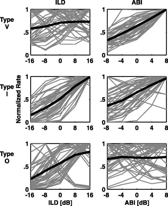
Normalized rate profiles of responses to the ABI/ILD stimulus set. Plotting conventions are the same as for Figure 4.

The type V units (Fig. 7, top row) display consistent increases in rate with increasing ABIs and a diverse range of response to ILDs. This result implies that the information provided about the ILD by type V units in their responses to the SN/ILD and ITD/ILD stimulus sets was mainly a response to the overall stimulus level, as opposed to a tuned response to midline azimuths as implied by Figure 4. For both stimulus sets shown in Figure 4, ABI peaks at the midline. The type V rate-profile results agree with the hypotheses of Ramachandran et al. (1999) and are consistent with the EE nature of type V units.

The type I rate profiles (Fig. 7, middle row) show a clear contralateral hemifield preference when using the ABI constant method, although in a few instances, there are mildly tuned responses to midline azimuths. This result is generally consistent with the data in Figure 4. Most of the cases studied here also show an increase in response with increasing ABIs.

The type O population again shows the most diverse rate profiles. Although the majority of units show a contralateral hemifield preference to ILDs, as in Figure 4, some neurons show a tuned ILD response, and in some cases, there are ipsilateral hemifield preferences. The response to increasing ABI shows no consistency in this population.

The representation of ABI-constant ILD cues is shown in Figure 8A. When the ABI is held constant, type I units carry significantly more ILD information than type V units (p < 0.01; rank sum). Conversely, MI_ABI (Fig. 8B) is higher in type V units than in type I units (p < 0.05; rank sum), and type V units have a larger ABI percentage (Fig. 8C) than type I units (p < 0.01; rank sum). The difference between type V and type O units is not significant in any of the three figures, although in each case, the type O units distribute more similarly to the type I units than to the type V units.

Figure 8.

The differential coding of the average level and level difference information. A, MI_ILD versus BF for the ABI/ILD stimulus set. B, MI_ABI versus BF. C, MI_ABI plotted against MI_ILD for each unit, expressed as a percentage of MI_FULL. Freq, Frequency.

The essentially binaural nature of the responses is demonstrated by the fact that MI_ABI is generally small (mean, 0.37 bits), most often <30% of MI_FULL (Fig. 8C) (most of the exceptions are type V units). In contrast, most MI_ILD measurements are larger (mean, 0.80 bits) (Fig. 8A), with values comparable with those given in Figure 5B. If neurons were truly monaural, MI_ABI and MI_ILD would be equal.

To explore how monaural or binaural sensitivity might contribute to the segregation of ABI and ILD coding, a histogram of the monaural indices computed for all of the units measured with ABI/ILD stimuli (Eq. 5) is plotted in Figure 9A. This index is 0 for binaural units, defined as equal sensitivity to sound level in both ears; it is +1 for units affected by the contralateral ear only and -1 for those affected by the ipsilateral ear only. As expected, this distribution is skewed toward positive values (contralateral sensitivity). There is some BF dependence to the monaural index, with values less than -0.2 only occurring for BFs ≤3 kHz (data not shown).

Figure 9.

Binaural sensitivity and coding. A, Histogram of monaural indices broken down by unit type. Values near 0 are the most binaural. Type O units cluster near 0, whereas type V units are more broadly distributed. B, MI_ILD is plotted against the absolute value of the monaural index, shown on a log scale. C, MI_ABI versus the monaural index. Mon Ind, Monaural index.

Surprisingly, the type O population turns out to show the most binaural sensitivity, with a tight cluster of responses around zero. The type V population, on the other hand, shows the least binaural sensitivity, having the most responses that approach 1 or -1. The absolute value of the monaural index can be used as a measure of the degree of binaural level interaction (with 0 being the most and 1 being the least). With this measure, the type V population has significantly less binaural interaction than either the type I or type O populations (p < 0.05; rank sum).

As expected, MI_ILD is largest in units with values of monaural index near 0 (Fig. 9B). Although MI_ABI (Fig. 9C) does not show much correlation with the monaural index, MI_ILD decreases almost linearly with the log of the monaural index. With one exception in the type V category, binaural units code ILD information much better than ABI information.

Discussion

Sound localization cues are segregated, to some extent, in brainstem nuclei: DCN neurons respond to SNs (Young et al., 1992) but not to ITDs and only weakly to ILDs (Young and Brownell, 1976; Joris and Smith, 1998); MSO neurons respond to ITDs but weakly to ILDs (Goldberg and Brown, 1969); and LSO neurons respond strongly to ILDs but weakly to ITDs (Joris and Yin, 1995). Of course, neurons in both MSOs and LSOs should respond to SNs, like any tuned neuron. Although quantitative comparisons cannot be done, our results suggest that localization cues are less segregated in the IC than in the brainstem nuclei. Given the hypothesis that IC response types are dominated by input from distinct brainstem nuclei, one expects to see similarities between LSO and type I units, DCN and type O units, and MSO and type V units. The limited segregation of localization cues expected on the basis of this hypothesis is not observed.

There is complete overlap in the type O and type I populations in the coding of ILD cues, despite weak ILD coding in the DCN and strong ILD coding in the LSO. SN cues are represented similarly in the type I and type O populations, and, in fact, there is slightly more information about SNs in the type I population, especially at BFs appropriate to notch sensitivity. This result is contrary to the suggestion that the DCN and type O neurons form a specialized channel for SNs (Young and Davis, 2002; Davis et al. 2003). Both type I and type O units encode ITD cues, which would not be expected from the characteristics of DCN or LSO neurons.

Unlike type I and type O units, type V units show properties similar to their hypothesized input from MSO neurons. They are sensitive to ITDs and ABIs (Goldberg and Brown, 1969) and relatively less sensitive to ILDs. They are not sensitive to SNs, but low BF neurons in general do not provide much rate information about SNs.

In summary, these results suggest substantial convergence of information across ascending pathways within the IC, especially for the type I and type O classes. This is consistent with the finding that type O units require a convergence of inputs with diverse properties to explain their responses to noise notches (Davis et al., 2003), although they have been shown to depend on inputs from the DCN for their primary properties (Davis, 2002).

It is possible that other classification schemes might result in a better segregation of localization cue information. However, the majority of units in this study respond to multiple cues, as shown by the percentage of units in Figure 6 that cluster toward the center of the plots. It is difficult to envision a classification scheme that would segregate these responses.

These results also suggest that studies aimed at the integration of localization cues in the IC will be profitable. The process of constructing the spatial location of sounds relies on varying degrees of cue integration, depending on conditions (Wightman and Kistler, 1992). In addition, particular cues may be useful in solving various discrimination problems: ITD cues are predominant in binaural unmasking, and SN cues are essential for elevation and front/back disambiguation. The relative reliability of ILD versus ITD cues depends on the frequency spectrum of the stimulus and the degree of reverberation. It is likely that the auditory system requires different degrees of convergence of localization cues in different conditions; the existence of neurons with widely varying degrees of cue integration, as suggested in Figures 6 and 8, would allow adaptation to different listening conditions and tasks.

Limitations of this approach

Because of the sparse sampling of the stimulus space, it is possible that the sensitivity of narrowly tuned units was underestimated. In general, however, units in the IC have fairly broad spatial receptive fields, with azimuth half-widths for tuned units averaging ∼60° (Aitkin and Martin, 1987; Delgutte et al., 1999; Sterbing et al., 2003). Furthermore, ITD discrimination thresholds for single neurons in the IC of guinea pigs have been estimated to range from tens to hundreds of microseconds (Shackleton et al., 2003), the range tested in this study. Although elevation per se was not tested, the SNs used represent elevations ranging in 7.5° steps from 0° to 30°. Units in the IC that show elevation tuning tend to have half-widths >20° (Aitkin and Martin, 1990; Sterbing et al., 2003). The range of parameters used should sample these receptive fields adequately.

Comparison with other studies

Only a few studies have looked at the effects of multiple cues simultaneously. Semple and Kitzes (1987) examined the interaction of ABI and ILD sensitivity in the IC of gerbils using pure tone stimuli, as did Irvine and Gago (1990) in cats and Wenstrup et al. (1988) in bats. The interaction of ITD and ILD sensitivity in the IC of cats has been investigated with clicks (Benevento and Coleman, 1970) and with tones and broadband noise (Caird and Klinke, 1987). Delgutte et al. (1995) manipulated virtual space stimuli directly to selectively target the effects of ITD and ILD cues on azimuth tuning. In general, these studies have found populations of neurons dominated by ILD cues, ITD cues, both cues, or neither cue. This study extends these results by quantifying sensitivity in terms of MI and correlating spatial response properties with frequency response maps.

Among studies that classified IC units in the same way as this study, Davis et al. (2003) looked at the processing of SNs in the type O pathway. They found that the majority of type O units showed an excitatory peak when a SN was slightly below the BF. In contrast, only some of the type O units in this study show an excitatory peak to the SN cue, with about one-half exhibiting a trough-like response. One possible explanation for this discrepancy is the limited sampling of SN center frequencies, because the study by Davis et al. (2003) sampled notches in a two-octave range around the BF compared with 0.2 octaves for this study. It is unlikely that this fully explains the differences, however, because the stimuli used here differed enough to produce significant rate modulations. Another possible explanation is that their study used straight-walled, full-depth notches embedded in otherwise white noise, whereas this study used more natural HRTF-filtered white noise.

Tollin and Yin (2002) showed that LSO azimuth tuning is primarily determined by the ILD in a narrow frequency band near the BF. In contrast to the results presented here for type I units, spectral shape did not determine a significant component of the responses in their study. This apparent difference probably derives from differences in the way SN stimuli were presented. Here, the spectra were shifted to center the SN frequency range on the BF, whereas Tollin and Yin (2002) used natural SN frequencies, which only occasionally aligned with the BF.

Individual HRTFs

The stimuli used in this study were based on HRTFs from Rice et al. (1992), despite the fact that Xu and Middlebrooks (2000) have found that precise spectral features of individual HRTFs vary across cats. This was done for two reasons. First, cats have mobile pinnae, and Young et al. (1996) have shown that HRTF shapes depend on pinna position. It is therefore difficult to ensure that even individual HRTFs would be appropriate, because one would have to ensure that internal proprioceptive information about ear position was appropriate to the SN stimuli (Kanold and Young, 2001). Second, there is a significant statistical disadvantage in using individual HRTFs for these experiments. The ultimate purpose of this study is to measure the sensitivity of units to sound localization cues, not sound location. As such, the stimuli were constructed to vary the localization cues over a constant set of values while minimizing other possible sources of variance, including those that might come from individual HRTF differences.

Interpretation of MI results

When using information theory to characterize neural responses, there are always questions of interpretation. It is worthwhile to stress that MI is a measure of neural sensitivity, not selectivity; this study does not provide insight into how information is functionally distributed across physiological classes. In other words, these results tell us where the information is, not how it might be used behaviorally.

Information analyses were important in obtaining the results in this study. For example, the rate profiles in Figures 4 and 7 show that type I units provide a simpler, more intuitive representation of both SNs and ILDs that is more uniform across the population than type O units. Nevertheless, there is little difference between the populations in terms of the information provided. Responses that are not systematic may still be useful to the brain in deciphering stimulus attributes. Stecker and Middle-brooks (2003) showed that a neural network model can extract spatial location from distributed codes in the auditory cortex. These codes need not be systematic in form; it is merely necessary that single units change their response when source location changes. Using MI to quantify neural sensitivity allows the identification of possible sources of information that do not take on a systematic form and might otherwise be overlooked.

Appendix

Here, a derivation of Equation 3 expressing MI_FULL in terms of MI_X and MI_Y is given. As shown in the study by Cover and Thomas (1991), the MI can also be expressed as a difference of entropies as follows:

(A1)

where the entropy H(Y) quantifies the uncertainty in the random variable Y and the conditional entropy H(Y|X) quantifies the residual uncertainty about Y, given knowledge of X. These entropies are defined in terms of the probability distributions as follows:

(A2)

Using the Chain Rule for information (Cover and Thomas, 1991), Equation 2 for MI_FULL can be rewritten as follows:

(A3)

where the conditional information is defined in terms of entropies as follows:

(A4)

Using Equation A1 to substitute for H(Y|X) in Equation A4 yields the following:

(A5)

The stimulus sets used in this study are designed such that MI(X; Y) = 0, because every combination of localization cues is presented an equal number of times. Ignoring this term, and substituting Equation A5 back into Equation A2 yields the following:

(A6)

which is exactly Equation 3.

References

- Adams JC (1979) Ascending projections to the inferior colliculus. J Comp Neurol 183: 519-538. [DOI] [PubMed] [Google Scholar]
- Aitkin LM, Martin RL (1987) Neurons in the inferior colliculus of cats sensitive to sound-source elevation. Hear Res 50: 97-105. [DOI] [PubMed] [Google Scholar]
- Aitkin LM, Martin RL (1990) The representation of stimulus azimuth by high best-frequency azimuth-selective neurons in the central nucleus of the inferior colliculus of the cat. J Neurophysiol 57: 1185-1200. [DOI] [PubMed] [Google Scholar]
- Aitkin LM, Anderson DJ, Brugge JF (1970) Tonotopic organization and discharge characteristics of single neurons in nuclei of the lateral lemniscus in cat. J Neurophysiol 33: 421-440. [DOI] [PubMed] [Google Scholar]
- Aitkin LM, Webster WR, Veale JL, Crosby DC (1975) Inferior colliculus. I. Comparison of response properties of neurons in central, pericentral, and external nuclei of adult cat. J Neurophysiol 38: 1196-1207. [DOI] [PubMed] [Google Scholar]
- Benevento LA, Coleman PD (1970) Responses of single cells in cat inferior colliculus to binaural click stimuli: combinations of intensity levels, time differences, and intensity differences. Brain Res 17: 387-405. [DOI] [PubMed] [Google Scholar]
- Boudreau JC, Tsuchitani C (1968) Binaural interaction in the cat superior olive S segment. J Neurophysiol 31: 442-454. [DOI] [PubMed] [Google Scholar]
- Brunso-Bechtold JK, Thompson GC, Masterton RB (1981) HRP study of the organization of auditory afferents ascending to central nucleus of inferior colliculus in cat. J Comp Neurol 197: 705-722. [DOI] [PubMed] [Google Scholar]
- Caird D, Klinke R (1987) Processing of interaural time and intensity differences in the cat inferior colliculus. Exp Brain Res 68: 379-392. [DOI] [PubMed] [Google Scholar]
- Cover TM, Thomas JA (1991) Elements of information theory. New York: Wiley.
- Davis KA (2002) Evidence of a functionally segregated pathway from dorsal cochlear nucleus to inferior colliculus. J Neurophysiol 87: 1824-1835. [DOI] [PubMed] [Google Scholar]
- Davis KA, Ramachandran R, May B (1999) Single-unit responses in the inferior colliculus of decerebrate cats. II. Sensitivity to interaural level differences. J Neurophysiol 82: 164-175. [DOI] [PubMed] [Google Scholar]
- Davis KA, Ramachandran R, May B (2003) Auditory processing of spectral cues for sound localization in the inferior colliculus. J Assoc Res Otolaryngol 4: 148-163. [DOI] [PMC free article] [PubMed] [Google Scholar]
- Delgutte B, Joris PX, Litovski RY, Yin TCT (1995) Relative importance of different acoustic cues to the directional sensitivity of inferior-colliculus neurons. In: Advances in hearing research (Manley GA, Klump GM, Köppl C, Fastl H, Oeckinghaus H, eds), pp 288-299. River Edge, NJ: World Scientific.
- Delgutte B, Joris PX, Litovski RY, Yin TCT (1999) Receptive fields and binaural interactions for virtual-space stimuli in the cat inferior colliculus. J Neurophysiol 81: 2833-2851. [DOI] [PubMed] [Google Scholar]
- Efron B, Tibshirani RJ (1998) Introduction to the bootstrap. Boca Rotan, FL: CRC.
- Geisler CD, Rhode WS, Hazelton DW (1969) Responses of inferior colliculus neurons in the cat to binaural acoustic stimuli having wide-band spectra. J Neurophysiol 32: 960-974. [DOI] [PubMed] [Google Scholar]
- Goldberg JM, Brown PB (1969) Response of binaural neurons of dog superior olivary complex to dichotic tonal stimuli: some physiological mechanisms of sound localization. J Neurophysiol 32: 613-636. [DOI] [PubMed] [Google Scholar]
- Guinan Jr JJ, Guinan SS, Norris BE (1972a) Single auditory units in the superior olivary complex. I: Responses to sounds and classifications based on physiological properties. Int J Neurosci 4: 101-120. [Google Scholar]
- Guinan Jr JJ, Norris BE, Guinan SS (1972b) Single auditory units in the superior olivary complex. II: location of unit categories and tonotopic organization. Int J Neurosci 4: 147-166. [Google Scholar]
- Imig TJ, Bibikov NG, Poirier P, Samson FK (2000) Directionality derived from pinna-cue spectral notches in cat dorsal cochlear nucleus. J Neurophysiol 83: 907-925. [DOI] [PubMed] [Google Scholar]
- Irvine DR (1987) Interaural intensity differences in the cat: changes in sound pressure level at the two ears associated with azimuthal displacements in the frontal horizontal plane. Hear Res 26: 267-286. [DOI] [PubMed] [Google Scholar]
- Irvine DRF, Gago G (1990) Binaural interaction in high-frequency neurons in inferior colliculus of the cat: effects of variations in sound pressure level on sensitivity to interaural intensity differences. J Neurophysiol 63: 570-591. [DOI] [PubMed] [Google Scholar]
- Joris PX, Smith PH (1998) Temporal and binaural properties in dorsal cochlear nucleus and its output tract. J Neurosci 18: 10157-10170. [DOI] [PMC free article] [PubMed] [Google Scholar]
- Joris PX, Yin TC (1995) Envelope coding in the lateral superior olive. I. Sensitivity to interaural time differences. J Neurophysiol 73: 1043-1062. [DOI] [PubMed] [Google Scholar]
- Kanold PO, Young ED (2001) Proprioceptive information from the pinna provides somatosensory input to cat dorsal cochlear nucleus. J Neurosci 21: 7848-7858. [DOI] [PMC free article] [PubMed] [Google Scholar]
- Kuhn GF (1977) Model for the interaural time differences in the azimuthal plane. J Acoust Soc Am 62: 157-167. [Google Scholar]
- May BM (2000) Role of the dorsal cochlear nucleus in the sound localization behavior of cats. Hear Res 148: 74-87. [DOI] [PubMed] [Google Scholar]
- Merzenich MM, Reid MD (1974) Representation of the cochlea within the inferior colliculus of the cat. Brain Res 77: 397-415. [DOI] [PubMed] [Google Scholar]
- Musicant AD, Chan JCK, Hind JE (1990) Direction-dependent spectral properties of cat external ear: new data and cross-species comparisons. J Acoust Soc Am 30: 237-246. [DOI] [PubMed] [Google Scholar]
- Oliver DL, Beckius GE, Bishop DC, Kuwada S (1997) Simultaneous anterograde labeling of axonal layers from lateral superior olive and dorsal cochlear nucleus in the inferior colliculus of cat. J Comp Neurol 382: 215-229. [DOI] [PubMed] [Google Scholar]
- Panzeri S, Treves A (1996) Analytical estimates of limited sampling biases in different information measures. Network: Comput Neural Syst 7: 87-107. [DOI] [PubMed] [Google Scholar]
- Park TJ, Klug A, Holinstat M, Grothe B (2004) Interaural level difference processing in the lateral superior olive and the inferior colliculus. J Neurophysiol 92: 289-301. [DOI] [PubMed] [Google Scholar]
- Phillips DP, Irvine DRF (1981) Responses of single neurons in physiologically defined area AI of cat cerebral cortex: sensitivity to interaural intensity differences. Hear Res 4: 299-307. [DOI] [PubMed] [Google Scholar]
- Ramachandran R, May BJ (2002) Functional segregation of ITD sensitivity in the inferior colliculus of decerebrate cats. J Neurophysiol 88: 2251-2261. [DOI] [PubMed] [Google Scholar]
- Ramachandran R, Davis KA, May BJ (1999) Single-unit responses in the inferior colliculus of decerebrate cats. I. Classification based on frequency response maps. J Neurophysiol 82: 152-163. [DOI] [PubMed] [Google Scholar]
- Reich DS, Mechler F, Victor JD (2001) Formal and attribute-specific information in primary visual cortex. J Neurophysiol 85: 305-318. [DOI] [PubMed] [Google Scholar]
- Reiss LJ, Young ED (2005) Encoding of rising spectral edges by neural circuits in the dorsal cochlear nucleus. J Neurosci 25: 3680-3691. [DOI] [PMC free article] [PubMed] [Google Scholar]
- Rice JJ, May BJ, Spirou GA, Young ED (1992) Pinna-based spectral cues for sound localization in cat. Hear Res 58: 132-152. [DOI] [PubMed] [Google Scholar]
- Rice JJ, Young ED, Spirou GA (1995) Auditory-nerve encoding of pinna-based spectral cues: rate representation of high-frequency stimuli. J Acoust Soc Am 97: 1764-1776. [DOI] [PubMed] [Google Scholar]
- Rose JE, Greenwood DD, Goldberg JM, Hind JE (1963) Some discharge characteristics of single neurons in the inferior colliculus of the cat. I. Tonotopical organization, relation of spike counts to tone intensity, and firing patterns of single elements. J Neurophysiol 26: 294-320. [DOI] [PubMed] [Google Scholar]
- Rose JE, Gross NB, Geisler CD, Hind JE (1966) Some neural mechanisms in the inferior colliculus of the cat which may be relevant to localization of a sound source. J Neurophysiol 29: 288-314. [DOI] [PubMed] [Google Scholar]
- Roth GL, Aitkin LM, Andersen RA, Merzenich MM (1978) Some features of the spatial organization of the central nucleus of the inferior colliculus of the cat. J Comp Neurol 182: 661-680. [DOI] [PubMed] [Google Scholar]
- Roth GL, Kochar RK, Hind JE (1980) Interaural time differences: implications regarding the neurophysiology of sound localization. J Acoust Soc Am 68: 1643-1651. [DOI] [PubMed] [Google Scholar]
- Semple MN, Kitzes LM (1987) Binaural processing of sound pressure level in the inferior colliculus. J Neurophysiol 57: 1130-1147. [DOI] [PubMed] [Google Scholar]
- Shackleton TM, Skottun BC, Arnott RH, Palmer AR (2003) Interaural time difference discrimination thresholds for single neurons in the inferior colliculus of guinea pigs. J Neurosci 23: 716-724. [DOI] [PMC free article] [PubMed] [Google Scholar]
- Stecker GC, Middlebrooks JC (2003) Distributed coding of sound location in the auditory cortex. Biol Cybern 89: 341-349. [DOI] [PubMed] [Google Scholar]
- Sterbing SJ, Hartung K, Hoffmann KP (2003) Spatial tuning to virtual sounds in the inferior colliculus of the guinea pig. J Neurophysiol 90: 2648-2659. [DOI] [PubMed] [Google Scholar]
- Strong SP, Koberle R, de Ruyter van Steveninck RR, Bialek W (1998) Entropy and information in neural spike trains. Phys Rev Lett 80: 197-200. [Google Scholar]
- Sutherland DP, Masterton RB, Glendenning KK (1998) Role of acoustic striae in hearing: reflexive responses to elevated sound-sources. Behav Brain Res 97: 1-12. [DOI] [PubMed] [Google Scholar]
- Tollin DJ, Yin TCT (2002) The coding of spatial location by single units in the lateral superior olive of the cat. II. The determinants of spatial receptive fields in azimuth. J Neurosci 22: 1468-1479. [DOI] [PMC free article] [PubMed] [Google Scholar]
- Treves A, Panzeri S (1995) The upward bias in measures of information derived from limited data samples. Neural Comput 7: 399-407. [Google Scholar]
- Wenstrup JJ, Fuzessery ZM, Pollak GD (1988) Binaural neurons in the mustache bat's inferior colliculus. I. Responses of 60-kHz EI units to dichotic sound stimulation. J Neurophysiol 60: 1369-1383. [DOI] [PubMed] [Google Scholar]
- Wightman FL, Kistler DJ (1992) The dominant role of low-frequency interaural time differences in sound localization. J Acoust Soc Am 91: 1648-1661. [DOI] [PubMed] [Google Scholar]
- Wise LZ, Irvine DRF (1985) Topographic organization of interaural intensity difference sensitivity in deep layers of cat superior colliculus: implications for auditory spatial representation. J Neurophysiol 54: 185-211. [DOI] [PubMed] [Google Scholar]
- Xu L, Middlebrooks JC (2000) Individual differences in external-ear transfer functions of cats. J Acoust Soc Am 107: 1451-1459. [DOI] [PubMed] [Google Scholar]
- Yin TCT, Chan JCK (1990) Interaural time sensitivity in medial superior olive of cat. J Neurophysiol 64: 465-488. [DOI] [PubMed] [Google Scholar]
- Young ED, Brownell WE (1976) Responses to tones and noise of single cells in the dorsal cochlear nucleus of unanesthetized cats. J Neurophysiol 39: 282-300. [DOI] [PubMed] [Google Scholar]
- Young ED, Davis KA (2002) Circuitry and function of the dorsal cochlear nucleus. In: Integrative functions in the mammalian auditory pathway (Oertel D, Fay RR, Popper AN, eds), pp 160-206. New York: Springer.
- Young ED, Spirou GA, Rice JJ, Voigt HF (1992) Neural organization and responses to complex stimuli in the dorsal cochlear nucleus. Philos Trans R Soc Lond B Biol Sci 336: 407-413. [DOI] [PubMed] [Google Scholar]
- Young ED, Rice JJ, Tong SC (1996) Effects of pinna position on head-related transfer functions in the cat. J Acoust Soc Am 99: 3064-3076. [DOI] [PubMed] [Google Scholar]