Widely Distributed Magnetoencephalography Spikes Related to the Planning and Execution of Human Saccades

Abstract

With sufficiently fast data sampling, ubiquitous sharp transients appear in magnetoencephalography (MEG) data. Initially, no known collective neuronal activity could explain MEG signal generation well above 100 Hz, so it was assumed that these transients were entirely composed of background electronic noise that could be eliminated by filtering and averaging. Recent studies at the cellular level provided evidence for synchronous synaptic input to dendrites and volleys of near-simultaneous action potentials. MEG studies have also identified high-frequency oscillations well above 200 Hz after averaging large number of somatosensory evoked responses. In this study, we searched for evidence of high-frequency neuronal activity in the raw MEG signal using the highest sampling rate available with our hardware. Two human subjects participated in three experiments using visual cues to define planning, preparation, and execution or inhibition of saccades. Tomographic analysis identified “MEG spikes” that were widely distributed across the cortex, cerebellum, and brainstem during cue presentations and saccades. Here we demonstrate how these MEG spikes can be recorded and localized in real time and show that task demands influence their properties. The MEG spikes were organized into feedforward and corollary discharge sequences that could, when combined with the slower activity-linked processing in discrete brain areas over long periods, lasting hundreds of milliseconds. Preparation for impending saccade began as soon as relevant information became available. Cues providing partial information initiated competing motor programs for as yet undecided future actions that were maintained until cues with new information resolved the uncertainty.

Introduction

After Dawson (1954) successfully isolated the evoked cortical potential by superimposing responses, averaging became the choice method for extracting useful signals from noisy data to reveal significant signals that are not readily identifiable in single trials. Averaging assumes that the signal can be separated into contributions evoked by the stimulus and noise from unrelated signals. However, recent results are challenging this assumption (Liu and Ioannides, 1996; Ioannides, 2001; Makeig et al., 2002; Laskaris et al., 2003), vindicating our suggestion that the average may be a “sandwich of histories” (Liu and Ioannides, 1996) and not one unitary sequence of events that repeats across trials.

The raw magnetoencephalography (MEG) signal shows peaks over 1 pT in amplitude, made up of large slow waveforms having smaller transients. These appear as irregular kinks with amplitudes ranging from tens to many hundreds of femtoteslas. Neuronal activity is not thought to be responsible for the sharpest, most fleeting events that last no more than a few milliseconds. We studied MEG spikes by analyzing single-trial MEG data using magnetic field tomography (MFT) (Ioannides et al., 1990) that built on two recent studies. The first used functional magnetic resonance imaging (fMRI) as the gold standard and showed localization of focal activity in the cortex with an accuracy of a few millimeters (Moradi et al., 2003). The second showed common saccade-related activation patterns in the cortex, cerebellum, and brainstem (Ioannides et al., 2004) that matched findings about nonhuman primate physiology (Keller, 1989; Lisberger et al., 1994). Activity from each gaze center was identified on either side of the brainstem. On each side, the direction of the current density vector before saccade onset changed consistently for saccades in the four cardinal directions. For each single trial, fast MEG activity was identified in the cortex and brainstem that was related to each other and to transients in the electrooculogram (EOG) in a task-dependent manner. We used a block design for saccade directions and a regular rhythm for each saccade and did not attempt to separate contributions attributable to planning, initiation, and execution of each saccade. To determine which part of the activity contributed significantly to the control of saccades, we teased apart these elements in the experimental design and used a fast sampling rate to record signals. We conducted three experiments. First, we used a detailed eye movement paradigm for one subject and isolated the three elements of eye movement using our standard sampling rate (1.6 ms) with an infrared eye tracker and EOG channels. Our results showed spike-like activity that changed too fast to be accurately described with the 1.6 ms MEG samples. Although the eye tracker was clearly useful to confirm EOG waveform, it also had disadvantages and provided no other information. The second experiment, using the same subject, took an important subset from the first experiment and used a fast sampling rate (0.48 ms). The third, with a new subject, used a fast sampling rate and EOG channels.

Materials and Methods

General background. Three separate basic neuronal events are likely candidates to generate a measurable magnetic field: action potentials traveling along the axon away from the soma, postsynaptic currents at the apical dendrites of neurons, and backpropagating spikes into the dendrites. A snapshot of an action potential in a myelinated axon shows sodium and potassium ion influxes separated by one node of Ranvier. The arrangement is a quadrupole with current dipoles 1 mm apart and pointing in opposite directions along the axon. From a fixed position along the axon, a propagating action potential appears as a rapid change of 100 mV in the membrane potential with a depolarization and repolarization spikes following each other within ∼1 ms. The repolarization is followed by the refractory period, an undershoot in the membrane potential that last for a couple of milliseconds during which the generation of a second action potential is inhibited. A single neuron can therefore generate only one action potential at a time. The next event is associated with current flows at the postsynaptic sites at the apical dendrites, which are relatively weak (∼10 mV) and slow (approximately tens of milliseconds). At any one time, many synaptic events can contribute to the activity of the same neuron, even if only a small fraction of the many thousand synapses are activated at any one time. It is possible that a sharp transient current is generated at the dendrites when significant number of inputs occur simultaneously. The third is backpropagating spikes that, under favorable conditions, drive a current from the soma into the dendrites. Whereas the strength and form of backpropagating action potentials depends on cell history and local membrane state, strength and duration are likely to fall somewhere between synaptic events and orthodromic action potentials.

Estimates for current density are ∼100 fA/m for current dipole moment of each dipole in the action potential quadrupole and ∼20 fA/m for a single postsynaptic event (Hamalainen et al., 1993). Even when more liberal estimates are used that increase the dipole moment by as much as an order of magnitude and allow a sizable fraction of synaptic events to contribute, the magnetic field generated by just any one neuron is still far below that which can be detected by MEG. To generate an observable MEG signal of ∼100 fT requires a current density strength that is at least many tens, possibly hundreds, times that produced by a single neuron. Finding the required number of neurons is easy, even in a tiny brain area well below a millimeter in diameter, but it is not enough. Elemental events do not add up constructively. Constructive summation requires temporal and spatial organization of the contributing neuronal population. Temporal organization, i.e., synchrony, is required to sum elemental events, and the vector nature of the magnetic field and the current density that generates it demands spatial organization, too. The MEG signal is a measure of the projection of the magnetic field vector along the normal direction to the sensing coil plane. Two nearby elemental sources with equal but opposite current density vectors generate the same MEG signal but with opposite signs, thus canceling the magnetic field of each other even at short distances. In a population with a large number of randomly oriented generators, the same number of current density vectors would point to any one of two diametrically opposite directions, so on average the same number could be found in any two opposite directions. Therefore, the strength and direction of the magnetic field generated by a population of randomly oriented elemental sources will be zero. In the brain, however, the current density of elemental events is not random because the shape of neurons dictates the intracellular currents and the architecture of the arrangements of neurons dictates the path of lowest resistance that extracellular currents follow. Put another way, the orientations of the neuron (its axon and/or dendritic arbor) and its neighbors determine the direction of the effective current density and the resulting magnetic field outside. A good arrangement for constructive summation is exhibited by large pyramidal neurons aligned perpendicularly to the cortical surface. An argument along similar lines suggests that action potentials are not good candidates for the generation of MEG signal. The two opposite dipoles in the quadrupole cancel each other out, at least in straight-line portions of the axon. It has therefore been assumed that action potentials do not contribute substantially to the generation of the MEG signal partly because of the current pattern they generate and partly because they are too fast to be synchronous. Excluding action potentials and ignoring the possibility of large-scale synchrony of elemental events led researchers to believe that no normal physiological processes generate a macroscopic MEG signal at frequencies above 100 Hz. Much of the thinking behind previous MEG studies was dominated by this view. Hence, high-frequency “contamination” continues to be routinely eliminated by averaging and/or filtering of the data. Slow postsynaptic events in the apical dendrites of pyramidal neurons are very likely generating that part of the MEG signal that remains after averaging and filtering the data below 100 Hz. However, theoretical considerations and accumulating evidence from invasive electrophysiological recordings and new imaging modalities for cellular neuroimaging suggest that a faster neuronal mechanism may also contribute to the MEG signal at frequencies well above 100 Hz.

Synchronous neuronal activity is increasingly being implicated in theories explaining the effective transmission of information in the brain (Abeles, 1991; Konig et al., 1996). Models of temporal jitter in excitatory and inhibitory synaptic input and of variability in spike output timing show how the rise time can remain equally sharp (on the order of 1 ms) over successive stages of processing in the striate and extrastriate visual cortex (Marsalek et al., 1997). Intracranial recordings in nonhuman animals support models of precise timing in neuronal firing patterns (Riehle et al., 1997) and synchrony in firing across many cells (Barth, 2003). New imaging techniques for large cell populations that use two-photon microscopy (Hubener and Bonhoeffer, 2005) show how precise spatial organization (Ohki et al., 2005) and temporal synchrony (Ikegaya et al., 2004) are in the neural machinery. Synchrony appears important for effective communication in the brain, but the studies do not show that this enhancement of high-frequency activity is enough to generate a measurable MEG signal. Recent biomagnetic recordings with special instrumentations have demonstrated that sodium spikes can be detected magnetically (and electrically), at least from in vitro preparations of longitudinal CA3 slices of guinea pig hippocampus (Murakami et al., 2002). Direct evidence for high-frequency brain activity (in the 200–800 Hz range) in humans was identified from EEG and MEG data for strong electrical stimulation of the median nerve (Haueisen et al., 2001). Often called high-frequency oscillations, this activity was identified after averaging many hundreds or thousands of trials. If such activity is strong but very brief and intermittent, then it might show as well, or even better, in single trials if the analysis can disentangle it from background noise. Later, we will describe very fast transient events, or MEG spikes, lasting just a few milliseconds, that are ubiquitous throughout the brain. These spikes are strong enough to be recorded and localized with MEG in real time. Moreover, they appear to reflect ongoing task demands, but they are not precisely time locked to any of these events.

It is necessary to augment the standard model for generation of the MEG signal guided by the recent evidence for massive synchrony to test these new ideas. Plausible mechanisms that may generate these high-frequency MEG signals may involve highly synchronous inputs at the synaptic level or synchronous discharge of action potentials. The usual arguments against action potentials can be easily fended off. Near the border of gray and white matter, axons bend sharply as they exit the gray matter, so the two dipoles of the quadrupole would momentarily appear on either side of the bend at an angle closer to 90° rather than 180°, a configuration that leads to strong MEG signal. These considerations coupled to the rapid changes in the MEG spike time course make action potentials more plausible candidates rather than slower synaptic events for MEG signal generation.

Subjects. Two right-handed healthy male subjects, 32 and 30 years old, with no history of neurological or psychiatric illness or drug abuse and normal visual acuity, binocular vision, and normal optic fundi participated in the MEG experiments. The first subject participated in two experiments, and the second subject participated in the third. The experimental procedure and the goals of the study were explained to the subjects who gave informed consent before each experiment. The RIKEN Research Ethics Committee approved the study.

Trial sequences and subject tasks. The two MEG experiments for the first subject (EXP1, standard sampling every 1.6 ms; EXP2, fast sampling every 0.48 ms) used runs with different sequences of stimuli designed to control cue information about the initiation of horizontal saccades. In EXP1, the subject was lying down and wore eye-tracker goggles with an incorporated stimulus screen, whereas in EXP2, he was sitting and looking at a translucent back-projection screen. For the second subject, in EXP3, fast sampling (0.48 ms) was used, and the subject sat in the same position as the first subject in EXP2. All cues used three kinds of symbols, which subtended 1° of visual angle (Fig. 1). A cross was always used for fixation, and it occupied either the center of the screen or was moved by 10° to either side. A square block marked possible target location of the next saccade and was either at the center or placed 10° on either side of the center or on both sides. A triangle was used to mark GO (up triangle), NOGO (down triangle), or saccade direction (left or right) and was presented at the current fixation point either at the center or moved by 10° to one side. For ease of reference, in Figure 1, the order of each cue in a trial sequence is denoted by a number on the bottom right of each box (both the number and box were not presented to the subject). Hereafter, we will use a number prefixed by cue (e.g., cue 3) to identify each cue. Cues providing information about the saccade (Fig. 1 B, cues 3, 6, 9) were presented for 500 ms, whereas all other linking cues (Fig. 1 B, cues 1–2, 4–5, and 7–8) were shown randomized between 1 and 3 s. A trial was defined by a complete sequence of cue presentations (Fig. 1 B, cues 1–9). A run was made up of 6–40 trials. Numbers of trials and runs are listed in Table 1. In each run, the trial order (Fig. 1 B, first saccades to left or right) was randomized.

Figure 1.

Stimuli and temporal sequences for control (type 0) and task runs (type 1–4) used in the saccade experiment. For details, see Materials and Methods. A–C, Types 0, 3, and 4 in EXP1, EXP2, and EXP3, respectively. D, E, Type 1 in EXP1. F, G, Type 2 in EXP1 and EXP3. For the results reported in this paper, we analyzed the MEG signal recorded around the onset of the cues highlighted in thick black boxes. Note that, for demonstration purposes, only the first saccade from center to right is shown in B, D, and F. During the experiment, the first saccade could be to the left or to the right, randomized within a run.

Table 1.

Recording details for EXP1 and EXP2 (subject 1) and EXP3 (subject 2)

Experiment	Notes	Recording order	Type	Number of sequences	Number of trials for each sequence	Total number of trials
EXP1, subject 1	With EOG and ET; supine position; SR, 625 Hz	Run 1	0	4	10	40
		Run 2	1	4	3	12
		Run 3	1	4	3	12
		Run 4	3	2	3	6
		Run 5	3	2	3	6
		Run 6	4	3	3	9
		Run 7	4	3	3	9
		Run 8	2	4	3	12
		Run 9	2	4	3	12
		Run10	0	4	10	40
EXP2, subject 1	No EOG/ET; sitting position; SR, 2083 Hz	Run 1	0	4	10	40
		Run 2	3	2	6	12
		Run 3	3	2	6	12
		Run 4	4	3	6	18
		Run 5	4	3	6	18
		Run 6	0	4	10	40
EXP3, subject 2	With EOG; sitting position; SR, 2083 Hz	Run 1	0	4	10	40
		Run 2	2	4	3	12
		Run 3	2	4	3	12
		Run 4	3	2	6	12
		Run 5	3	2	6	12
		Run 6	4	3	6	18
		Run 7	4	3	6	18
		Run 8	0	4	10	40

In each run, the sequences were presented randomly. SR, Sample rate.

The main experiment consisted of several runs of types 1–4. Control runs were introduced before (pre-EXP) and after (post-EXP) the main experiment. These control runs were of type 0. In these control runs, the symbols carried no experimental meaning because the subject viewed them passively. Figure 1 A shows the sequence of stimuli for control, type 0 runs: cue 1, central cross; then cue 2, 10° blocks and cross; finally, cue 3, 10° blocks and a central triangle pointing left or right, or up or down.

Figure 1, B and C, shows the next two types of runs, type 3 and type 4. Cues 1 and 2 were identical for both types 3 and 4 runs. Type 3 consisted of GO trials only, whereas type 4 had GO and NOGO trials intermixed. For types 3 and 4 GO trials, cue 3 was a central left- or right-pointing triangle. When this cue appeared, the subject immediately made a saccade of 10° in the direction of the cue triangle and held their eyes there until cue 6 appeared. For type 4 NOGO trials, cue 3 was a central downward-pointing triangle (Fig. 1C).

Finally, the two remaining types, types 1 and 2, were used to disentangle the direction (D) and the command to move or not (M). In these two cases, the final command initiating the sequence of saccades was given after the nature of the saccade was completely defined by earlier direction (D) and move (M) cues. For type 1 (Fig. 1 D, E), the stimuli were as follows: cue 1, central cross; cue 2 (direction cue D), central triangle pointing to the direction to be made; cue 3, central cross and blocks; cue 4 (move cue M), upward-pointing triangle GO or downward-pointing NOGO trial; cue 5, central cross and blocks; and cue 6 [cue to initiate action (A)], a left- or right-pointing triangle in the direction of D. For a GO trial, the subject had to execute the saccade as soon as possible after action cue 6 by moving their fixation from the center to 10° to the block in the direction defined by D. For a NOGO trial, the sequence ended at cue 6 with no eye movement. For type 2, the stimuli and the sequence were the same as for type 1, except cue 2 and cue 4 (D and M) were reversed. In both type 1 and type 2 runs, the subject knew whether or not to move and in which direction for seconds before the action cue 6 was delivered.

In GO trials, each saccade initiated by the first action cue of the trial as described above was followed by a standard sequence of additional saccades that went automatically through the following steps: Cues 4–9 for types 3 and 4 (Fig. 1 B) and cues 7–12 for types 1 and 2 (Fig. 1 D, F). In NOGO trials, the trial ended at cue 3 for type 4 (Fig. 1C) and at cue 6 for types 1 and 2 (Fig. 1 E, G).

In Figure 1, we used thick black boxes to outline the periods used for data analysis leading to the results reported in this paper. Specifically, we analyzed activity elicited by the action cues initiating or demanding inhibition of the first saccade for all available cases of EXP1 (types 1, 2, 3, and 4), EXP2 (types 3 and 4), and EXP3 (types 2, 3, 4) and for all control stimuli (pre-EXP and post-EXP). We also analyzed the activity elicited by cue 4, the setting of direction cue, in type 2 GO/NOGO trials in EXP1 and EXP3. For type 2, the GO/NOGO cue 2 was given first, 1–3 s before the saccade direction cue 4, and then the action cue 6 followed 1–3 s after cue 4. Therefore, when cue 4 was presented to the subject, he knew whether the trial was GO or NOGO and he was just informed which direction the saccade should be made (in GO trials), but he was not to make any saccade for the next 1–3 s until cue 6. Therefore, brain activity observed just after cue 4 (in type 2 GO trials) is related to processing of information about saccade direction and is free from any large activity that saccade execution may introduce.

MEG, EOG, eye-tracking, and electrocardiogram recordings. EXP1 and EXP2 were performed on different days on the same subject, whereas EXP3 was performed on another subject. The MEG signal was recorded with a whole-head 151-channel system (CTF Systems, Vancouver, British Columbia, Canada) inside a magnetically shielded room. In EXP1, data were sampled at 625 Hz (1.6 ms) with low-pass filtering at 200 Hz. In EXP2 and EXP3, data were sampled at 2083 Hz (0.48 ms) with low-pass filtering at 600 Hz (the upper limit of 600 Hz is imposed by the MEG acquisition hardware). In EXP1, eye movement was monitored by the horizontal and vertical EOG and an infrared eye-tracking system housed in goggles (Avotec, Jensen Beach, FL). The continuous eye monitoring of the mechanical motion of the eye during the MEG signal recording was demanding because frequent recalibration of the eye tracker and head position were necessary to compensate for occasional loss of image. The sampling rate provided by the eye tracker was also limited to 60 Hz, which was well below that of the MEG signal (625 Hz). Eye movement monitoring therefore consisted of two fast records (the MEG and EOG signal) and a slower record from the eye tracker. Binocular fusing of the independent goggle screens required effort, so convergence effects could not be avoided. EXP2 solved this problem by using a screen presentation without EOG or goggles, and EXP3 was similar but used EOG. In EXP1 and EXP3, the subject's heart function was monitored using four pairs of electrocardiogram (ECG) electrodes placed on the left and right wrists, left and right ankles, and lead V2. For EXP2, one pair of ECG electrodes was placed as for lead V2.

Signal processing. Off-line, environmental noise was first removed from the raw single-trial data by forming the third gradient of the magnetic field and notch filtering (50 Hz and its harmonics). In EXP1, three trials with eye blinks as indicated by EOG and eye tracker around saccade onset were rejected: one trial each from type 3, run 4, and type 1, runs 2 and 3. In EXP3, one trial was rejected from type 4, run 6. Independent component analysis (ICA) (Jahn et al., 1999) was then applied to remove subject artifacts such as heart function as recorded by ECG. ICA also identified eye-movement-related activity, but these components were not removed.

Tomographic analysis. Simple point-like descriptions of generators can usually explain the average MEG data evoked when simple sensory stimuli are repeatedly presented, but results using such models and data averaging can be mis-leading (Ioannides, 2001). We used MFT (Ioannides et al., 1990) to extract tomographic estimates of activity from single-trial MEG data. MFT produces probabilistic estimates for the nonsilent part of the primary current density vector J(r, t). Although MFT exploits forward problem linearity, it relies on a nonlinear algorithm to obtain a distributed solution for sparse and compact current densities in the brain (Taylor et al., 1999). Numerous recent studies have demonstrated that MFT analysis can identify evoked responses in single trials (Liu and Ioannides, 1996; Ioannides, 2001; Liu et al., 2003). Our MFT analysis followed the same procedure as our previous studies, using four separate source spaces to cover the left, right, superior, and occipital parts of the brain. In addition, fifth source space was added for the anterior part of the brain that included eyes and ocular muscles. The left and right source spaces were enlarged to allow for coverage of the orbit. The results from the five source spaces were combined into one large source space covering the entire brain.

Localization accuracy and depth sensitivity. How precisely MEG can localize has been hotly debated for many years. In a real experiment, MEG signals are generated by patterns of generators that change continuously from trial to trial. The question of localization accuracy, therefore, must be addressed within a statistical framework and for biologically realistic conditions. We recently tested MFT localization accuracy by measuring activity elicited within a small part of V1 using identical stimuli with the same subjects in fMRI and MEG (Moradi et al., 2003). This study demonstrated localization accuracy of ∼3 mm at cortical level.

Accurate localization for superficial generators does not automatically imply good localization for deeper sources. Deep generators produce weaker MEG signals, first, because of the inverse power law that relates strength of magnetic field and the distance to the source, and, second and more critically, because sources very close to the center of a conducting sphere, like the head, produce no external magnetic field. Because the cerebellum and brainstem, the two deep generators of interest in the present study, are well away from the center of the head, it is the distance from the sensors that will weaken their contributions. Compared with superficial generators (e.g., in V1), the MEG signal from the cerebellum and brainstem is approximately one order of magnitude less, well within the dynamic range of modern MEG hardware. The noise level of our MEG system is below 10 fT, i.e., two to three orders of magnitude below the range of typical single-trial MEG signal. It is therefore expected that, although the localization of deep generators would not be as good as for superficial ones, the deterioration would be moderate. Recent MEG studies from our group (Ioannides et al., 2004) and others (Hashimoto et al., 2003; Tesche and Karhu, 1997) have reported such activity in the brainstem and cerebellum. A review of MEG studies of cerebellar activity with emphasis on recent real-time reconstructions using the techniques used in this work can be found elsewhere (Ioannides and Fenwick, 2005).

Properties of current density vectors. For the computation of sensor sensitivity profiles (lead fields) needed for the MFT analysis, a separate sphere model was used with center chosen to fit optimally the inner surface of the skull for each individual source space. For a spherical conductor, the radial direction is silent, i.e., any current element pointing along the direction joining its position and the center of the conducting sphere produces no magnetic field outside the conductor. By construction, the MFT solutions for each of the five source spaces produce a current density vector J(r, t) without any radial component. Because different sphere centers are used for each of the five source spaces, there is no single radial direction and hence no completely silent direction. Nevertheless, because the human head is nearly spherical, the direction from the center of the head to a given point on the cortex is almost a silent direction, so non-zero values for J(r, t) are almost entirely confined to the local tangential plane. This plane contains the point r, and its local normal is along the direction from the center of the head to r.

Current density units. The nonlinear nature of MFT allows for changes in the lead fields at different sensor locations in different runs. The MFT algorithm uses a regularization step to resolve the conflicting requirements of high spatial accuracy and insensitivity to noise (Ioannides et al., 1990). The strength of the current density is effectively renormalized by an arbitrary constant that fixes how much a point-like generator will be spread in the reconstruction. The precise value of the renormalization constant depends on the level of noise in the data and the relative contribution of intracellular and extracellular currents, i.e., fine details of local geometry that have a minimal effect as long as one is not interested in microscopic details. The actual value of the overall normalization does not affect relative changes of activity either in time or across different conditions and stimuli. We therefore present the MFT results in arbitrary units acknowledging the uncertainty in determining this overall normalization constant.

Data used in tomographic analysis. For EXP1, we analyzed trial segments 1 s before and 1 s after cue onset, making 1250 time slices for each single trial analyzed. We analyzed this long period because our previous eye-movement study showed that activity related to saccade planning, preparation, and execution extended to many hundreds of milliseconds before and after saccade onset. Eye movements were identified independently from the EOG and eye tracker. Only the EOG was used to define the saccade onset in EXP1 and EXP3. Because EXP2 did not have EOG electrodes or eye tracker, the precise time of saccade onset, after detailed visual inspection of the frontal MEG channels, was marked by hand and verified by an independent rater. For EXP2 and EXP3, the data around the saccade were analyzed, from 200 ms before to 500 ms after saccade onset, yielding 1458 time slices per single trial. A tomographic image was obtained for each time slice of the above single-trial MEG data.

Pattern analysis. The availability of a very large number of MFT solutions millisecond by millisecond provides an opportunity to apply powerful pattern analysis techniques (Laskaris and Ioannides, 2001). At each time slice t for each trial and condition (collectively identified by the index i), a pattern X_i(t, p; Δt) is defined over a time window of w = p ×Δt. It consists of p samples around t, spaced Δt units from each other (Δt is an integer multiple of the original time step in the data). Specifically,

The samples x_i(t) are single value scalar quantities (e.g., the projection of the current density vector along a given direction), a vector (e.g., the current density vector at a given point in the source space), or a collection of vectors (e.g., the full vector field defining the MFT solution at a given time slice). With considerable computational effort, the application of pattern analysis on sets of patterns X_i produces time-dependent measures that either summarize regional activity across a set of single trials of a given condition or contrast the single-trial responses between conditions. Some of these methods reduce to conventional approaches such as ensemble averaging and measures of signal power (SP) when individual responses are used instead of patterns of data.

Data summaries for one-type time-locked responses. Two kinds of markers can be used to search for time-locked events in the single trials. The onset of any one of the visual cues can be used to align single trials and seek activations that recur at similar latencies relative to the cue onset. The beginning of saccades, as defined by the EOG onset, can also be used to align single trials and look for time-linked activations before and after saccade initiation. We have shown previously that very different kinds of information can be obtained from the same data after aligning single trials to the onset of either visual or auditory cues or to movement (Ioannides, 2001). For the control runs only, image onset is available as a marker, whereas for the task runs, both image ONset (I-on) and saccade ONset (S-on) are available. S-on alignment is only available for GO trials at action cues when a saccade is executed. After alignment, the current density vector in different single trials can be processed in a number of conventional ways. Here, we use three data summaries, namely, averaging, statistical parametric mapping (SPM), and signal-to-noise ratio (SNR) computations.

Averaging. In this case, the aligned MFT solutions are averaged across single trials at each source space point (voxel). Either the current density vector or its modulus can be averaged. Additional smoothing (over latencies) makes the results less sensitive to time jitter across single trials.

Statistical parametric mapping. Because the MFT computation for each time slice is performed independently, we can treat the modulus of the current density vector at each time slice as an independent random variable and apply post-MFT SPM analysis (Ioannides, 2001). Specifically, following the same voxel-by-voxel procedure used for fMRI data analysis, we applied SPM analysis using t test to compare MFT solutions between an active and a baseline condition or between two active conditions. The SPM analysis is used to identify statistically significant changes in activity over the aligned segments of data. For saccade onset, the statistical comparison was made between two conditions (Fig. 1 B, between the saccade right cases for types 3 and 4, as shown in cue 3). For cue image onset, the comparison was made between an active condition and control runs (pre-EXP and post-EXP) with identical visual cues (Fig. 1, between the saccade right cue 3 in B and the visual cue 3 in A). The SPM analysis uses MFT solutions from a time window covering a finite range of latencies. This window can be just a few milliseconds across and stepped every time slice or many hundreds of milliseconds across and stepped every hundred or more milliseconds. A long window allows for latency jitter at the expense of time resolution and insensitivity to sharp transient events. A short window offers better time resolution, but it misses changes in activity with latency jitter comparable with the window size. Both long and short windows will miss changes between active and baseline distributions if the variance in the active condition is high because of changes as the run progresses (e.g., habituation).

Signal-to-noise ratio. The signal content of the ensemble of single trials is quantified using an SNR estimator with a moving window. First, single trials are aligned with respect to either S-on or I-on. Then a window is defined around each time t relative to the alignment time. In terms of the notation established above, the average signal (X̄), SP, noise power (NP), and SNR for this window are defined as below (Laskaris and Ioannides, 2001):

The average X̄ is the ensemble average of N single-trial patterns, each with p samples. The noise power NP is the ensemble average of single-trial deviations from X̄, computed with the L₂ norm. The signal power SP is the noise-corrected L₂ norm of X̄. The SNR can be thought of as the ratio of the “energy” in the reproducible part of the signal divided by the “energy” of the residual signal across single trials.

Simple identification of regions of interest. The definition of a region of interest (ROI) is simple when a stimulus evokes strong activity in a primary sensory area because the early response is focal and it is usually associated with one dominant current density direction. In such cases, consistently activated SPM loci correspond to the expected anatomical landmarks defined on the subject's structure MRI. Invariably, Talairach coordinates (Talairach and Tournoux, 1988) of these SPM foci are consistent with what have been reported in the literature by other methods. The direction of the dominant current density can then be simply read off from the direction of the local current density at the peak of the average of the single trial MFT solutions.

Location of gaze center ROIs was simpler in our previous study, because blocks of saccades in the same direction were executed continuously with a regular tempo once every 4 s (Ioannides et al., 2004). The regular rhythm used in that study was reflected in the stereotyped activation of gaze centers on each side of the brainstem, producing coherent activity across trials and prominent vector averages that also changed polarity around saccade onset. In that study, the activation in the last 100 ms before saccade onset, initiated by an auditory cue (providing a clear time-locking signal) was strong compared with control periods of many hundreds of milliseconds and regular enough to produce clear SPM foci at the gaze center on the ipsilateral side to the saccade direction for horizontal movements. In the same period, just before saccade onset, the current density direction was consistent across single trials at the foci identified by SPM, allowing the definition of both the location and the main direction for the ROI.

In the present study, two opposite current directions were again identified in each gaze center for all three experiments. However, the saccade direction was randomized within each run, and thus the subject was unaware which direction the saccade should be until a trial started. As a result, in the presaccadic period, there were two candidate directions that elicited a complex pattern of activation in both the brainstem and frontal eye fields (FEFs), particularly for the first subject (EXP1 and EXP2). With two predominantly opposite current density directions active in the same time period, aligning the single trials based on either image or saccade onset did not always result in the visualization of clear focal activations in either the cortex or gaze centers. For these cases, the more elaborate strategy described below was used for the definition of ROIs.

Data summaries for multiple-type time-locked responses using circular statistics. When a unimodal distribution is present and latency jitter is small, averaging across single trials can isolate significant patterns. Averaging is ineffective in the presence of latency jitter, or still worse if current density vectors are in nearly opposite directions at similar latencies across single trials or there are changes of vector direction in quick succession in the same trial. Averaging is particularly ineffective for spikes because of their short-lived and intermittent nature. We anticipated that different types of single-trial responses would correspond to different current density directions. Because the current density vector contributing to the MEG signal is essentially confined in two dimensions, its variation can be conveniently quantified and displayed using circular statistics (Fisher, 1993). Circular statistics provides an established framework for the identification of statistically significant distributions based on both the magnitude and direction of current density vectors within a finite time range, which can be many hundreds of milliseconds long, and/or across single trials and conditions. The ROI activation for each single trial is inspected and all peaks in the target latency range are identified. The strength of each peak is rescaled by dividing by the overall maximum value (strength of the strongest spike in the latency range). Peaks with relative strength above a predefined relative threshold (usually set to 0.5) are selected and their directions are noted. The selected instantaneous peaks are then used in the circular statistics and displayed as circular diagrams. In the circular diagram, each MEG spike is represented by a line in a polar plot. The line length represents the (relative) peak amplitude of each identified MEG spike and its polar angle the direction of the current density vector at the peak relative to some reference direction. Because numbers of peaks in any single trial are not equal, there will not be equal numbers of lines in the graphs of circular statistics from different ROIs, trials, or at different latency ranges from the same ROI. In a circular diagram, maxima (of slow activity or MEG spikes) with amplitude at least half as strong as the maximum in the range are shown together with the probability density function (PDF) obtained after smoothing across the identified maxima. A χ² criterion is used to determine whether the PDF departs significantly from uniform distribution, and, if so, the significant directions are defined and shown as white arrows on the circular statistics diagram. The graphical representations of the results of circular statistics analysis are easy to interpret because statistically significant recurring patterns show up as easily recognized features.

Endogenously generated organization analysis. For capturing and quantifying spikes in brain activations, we used an analysis strategy that we called endogenously generated organization (EGO). EGO analysis naturally follows from the results of circular statistics. A significant direction is first selected to describe the activity of a given ROI. Matching activations (peaks of activity in the given ROI along the selected direction) are then sought across single trials within a latency range (usually the same range used for the circular statistics). For each match, a sequence of MFT solutions is cut from the single trial centered at the identified peak latency. The average of these EGO aligned segments of MFT solutions provides a measure of the evolution of activity throughout the brain around spikes in the given ROI with the selected direction. In this paper, we will characterize spike activity along a selected direction in terms of the time course in the given ROI extracted from the average of the corresponding EGO-aligned MFT solutions.

Complex identification of regions of interest. A more elaborate strategy was used to identify activity that recurred with similar strength and in very similar directions intermittently across single trials but did not survive averaging because of strong activations in the opposite direction. For example, the SPM analysis using long windows for the first subject did not always produce clear foci of activity in the gaze centers and frontal eye fields. For these more complicated cases, we used anatomical definitions and the SPM loci if available as general guides for a preliminary definition of ROIs. The precise location was then defined by visual inspection of instantaneous single trial MFT solutions. The main direction of the current density vector for each ROI was defined as the direction found at the peak of the vector average of the relevant condition. If the peak in the vector average was not distinct, circular statistics analysis was used to define the main direction.

Definition of agonist and antagonist directions for gaze centers. The definition of a single main direction for each ROI allows a gross comparison between conditions. For a more detailed analysis of the gaze center activity, we used circular statistics to define directions using the current density vector between 30 and 60 ms after saccade onset. We know that, during a saccade, in the gaze center the agonist abducens nucleus fires strongly, whereas the antagonist nucleus reduces its activity (Leigh and Zee, 1999). During this period, the current density vectors of each gaze center were clustered around a single dominant direction that was different, as would be expected on the agonist or antagonist sides of the gaze centers and for each saccade direction.

Assuming that the degree of orderly activations in a presaccade time window reflects the state of preparedness for an impending saccade, we can obtain a measure of the completeness of eye-movement preparation before saccade onset by circular statistical analysis of the primary current density directions across single trials for each gaze center at this time. Completed preparation would be indicated by a distribution with a sharp maximum in the agonist direction for the ipsilateral gaze center and in the antagonist direction for the contralateral gaze center. Maintenance of plans for both possible movements would be shown by the presence of strong peaks along both agonist and antagonist directions. A rather diffuse distribution would indicate that either preparation was incomplete or this ongoing state was not reflected by gaze center activity as captured by MFT analysis.

Circular statistics for frontal eye fields. Circular statistics analysis was also performed for FEFs. For the FEFs, the activity related to saccades was identified for hundreds of milliseconds both before and after saccades, corresponding to preparation and planning and to corollary signals, respectively. This complexity prevents a clear definition of one direction as agonist or antagonist, so we simply used circular statistics as a tool for displaying different modes involved and their temporal evolution around cue and saccade onset in different conditions.

Mutual information analysis. Mutual information (MI) (Shannon, 1948) is used to examine how activity between different brain areas is linked. MI is computed between two time series linking single-trial activations in one ROI at t with another ROI at t + τ, where τ is the delay time between second and first ROIs (Ioannides et al., 2000). Each time series is a pattern defined within a window of width w = MI_w. The full MI map is constructed by running each window at a step MI_s, for latency t and delay τ. The standard definition of MI assigns equal weight to all couplings. A reasonable starting point would be to emphasize the strongest couplings between areas of the brain using the Renyi generalization that allows the assignment of different weights (Renyi, 1970). In this work, we used the Renyi generalized mutual information with q = 4, as we have done in all of our previous MI studies. This choice produces a coupling profile that emphasizes the strongest links but yet also allows weaker ones to be seen. A fuller description of the MI analysis, including the Renyi generalization and an intuitive interpretation of its meaning, can be found elsewhere (Ioannides et al., 2000).

Influence diagrams are derived from MI maps by drawing an arrow for each identified feedforward and feedback link between two areas, using the same procedures as in our previous study of human saccades (Ioannides et al., 2004). A high MI value does not necessarily imply a causal influence. The link identified by a high MI value may be attributable to common interaction with a third area via links with different time delays. Assuming that axonal conduction time plays an important role in the observed MI results, direct linkage is more likely to be reflected in MI values with delays as small as the fastest monosynaptic contacts may allow, e.g., 4–8 ms between areas known to be directly linked by fast well myelinated axons and separated by a few centimeters. Only the MI computations with small window segments from EXP2 have the time resolution (sampled every 0.48 ms) to deliver such information. The mechanism responsible for the very strong dominant linkages with long time delays is likely to be very different.

If a control condition is present, then the MI values in the control condition can be used to define a threshold for significance. When no control condition is present, the relative threshold can be defined so that only the peaks of MI survive. This simple procedure is surprisingly effective, as demonstrated below by computing the MI using the time series from the horizontal EOG (EOG-H) and horizontal eye tracker (ET-H) data.

Results

EOG and eye-tracker data analysis

Figure 2 shows how information about eye movement is represented and analyzed and why effects of windowing are important in the analysis of data with rapidly changing signals. The examples use the EOG and eye-tracking data from EXP1 runs of types 3 and 4 (GO), cue 3, saccade from center to left or to right. Averages for the horizontal EOG and for the eye-tracker data are shown in Figure 2, A and B. The averages were produced by aligning the single trials to image onset (Fig. 2A) and saccade onset (Fig. 2B). The limitations of the eye tracker are evident in the more stepwise appearance of the graph because of the slower sampling rate (60 Hz). Figure 2, C and D, shows the effects of windowing on SNR and MI using the EOG-H and eye-tracker data aligned to saccade onset from type 3 (GO), center to left saccades in EXP1. Figure 2C shows signal power, noise power, and signal-to-noise ratio at 5 ms (yellow), 40 ms (blue), 96 ms (green), and 200 ms (red) windows. Signal power increases steadily over time, changing little as window length changes. In contrast, the noise power fluctuates strongly, creating the dominant features of SNR. Also, the spreading introduced by longer windows of 96 and 200 ms extends before saccade onset and blurs the fine details seen only in the 5 ms window. The feature at 10 ms after saccade onset (highlighted by the dotted ellipse in Fig. 2C) illustrates this. This apparently small feature corresponds to a very high SNR value (30). This SNR peak marks the start of the ballistic movement. In our protocol, the subjects would fixate on the 10° side blocks following the initial saccade away from the center, so a high, nearly constant EOG level is established at the end of the saccade (after ∼80 ms) generated by the displaced dipole field of the corneo-retinal potential. The corresponding signal power settles at high values, reflecting the nearly constant and high EOG level, but fluctuations in the much smaller noise power in the denominator generate very prominent SNR variations. The left side of Figure 2D shows a mutual information map computed from the time-lagged segments of horizontal eye tracker against EOG using the same GO trials as in Figure 2C. The line, shown at 45° through zero (the iso-ocular line), marks all events that have an influence on the eye-tracker at time 0 (the start of the movement of the globe) and separates events occurring before (to the left of the iso-ocular line) and after (to the right) the globe started its movement. The time on the horizontal axis denotes the actual time of the linked event in the EOG. Positive eye-tracker delay (vertical axis) corresponds to links in which the EOG events led eye-tracker events, whereas negative eye-tracker delay indicates where EOG events follow. The map shows the effects of windows MI_w = 48 ms (red), 96 ms (blue), 200 ms (green), with steps MI_s = 4.8 ms. With the MI threshold set to 0.5, no islands survive in the presaccadic period. The red dashed outline shows the MI island that survives with the lower threshold of 0.2. This MI island links ocular muscle activity 200 ms before the saccade (as marked by the EOG) to the beginning of the globe movement (as marked by the eye tracker). This MI island can only be seen in the shortest window of 48 ms and may reflect muscular adjustment ∼100 ms after image onset preparatory to the movement. The right side of Figure 2 D shows the influence diagram derived from the MI map. On the influence diagram, the top row is the EOG, whereas successive rows are for the eye tracker using different windows with time flowing from left to right. The figure shows bidirectional influences, illustrated by a double-headed line, between horizontal EOG and the eye tracker clustered around saccade onset (time 0). The bidirectional influence follows from the spread of the corresponding contours in the MI map both above and below the zero line of the eye-tracker delay. The length of the horizontal black bars in the EOG and eye-tracker rows represents the duration of linked activity in the EOG and eye-tracker time series. The dashed red link shows the influence, using the short 48 ms window, from the EOG-H 200 ms before saccade onset to the eye tracker after eye movement. In summary, Figure 2 D shows information at two distinct timescales, depending on the windowing used for the MI computations. Fast activity in the EOG relating transients in the ocular muscles to the slow movement of the globe hundreds of milliseconds later can be seen only with the smaller 48-ms-long window. Longer windows are dominated by slow components and reflect events occurring within similar timescales, such as the EOG response to the dipole displacement as the globe moves.

Figure 2.

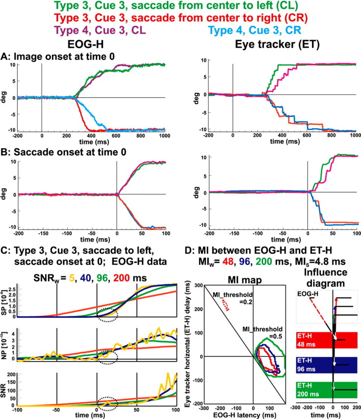
The analysis methods used in this study: averaging, SNR, and MI analysis using EOG-H and ET-H data. A, B, Averaging on image onset (–200 ms to 1 s) and on saccade onset (–200 to 100 ms), respectively, for EXP1 types 3 and 4, GO trials, cue 3. The different colors correspond to different conditions of cue 3, e.g., green is for type 3 saccades from center to left (CL). C, D, Windowing of SNR and MI analysis. C, Bottom, SNR; middle, NP; top, SP. Data from EOG-H, EXP1, type 3, cue 3, saccade CL with SNR windows 5 ms (yellow), 40 ms (blue), 96 ms (green), and 200 ms (red). D, MI map (left) and its influence diagram (right). The MI map derived from EOG-H and ET-H time series from the same data as for SNR in C. Iso-ocular line (45° through 0) corresponds to events coinciding with eye tracker at time 0. MI threshold was set to 0.2 before and 0.5 after saccade. MI maps with windows MI_w = 48 ms (red), 96 ms (blue), and 200 ms (green) are compared using the same step MI_s = 4.8 ms. Note that only the shortest 48 ms window shows the linked activity between EOG-H 200 ms before saccade and eye tracker after saccade (dotted red line).

Regional brain activations

The simple ROI definition using SPM and vector average data were sufficient to localize V1/V2 and cerebellum (flocculi and vermis). For each subject, bilateral V1/V2 ROIs were defined by the activity in the visual cortex using stimuli in the control runs between 65 and 80 ms. The flocculi and vermis ROIs were defined by activity soon after saccade onset, GO condition, from types 3 and 4 data. For the second subject (EXP3), focal changes in the long window SPM analysis and MFT vector averages showed clear foci in the cortex and brainstem to define the ROIs of frontal eye fields and gaze centers. For the first subject (EXP1 and EXP2), two candidate directions were equally strong and produced complex activation pattern in the vector averages and few SPM foci. These SPM loci were used as general guides for ROI definition of the gaze centers and frontal eye fields. The precise definition was obtained from consistently strong single-trial activations 100–200 ms before saccade onset, identified by both visual inspection and circular statistics analysis. Talairach coordinates for the centers of all ROIs used in this paper are listed in Table 2. The coordinates were close to those identified in our previous study for the gaze centers and frontal eye fields (Ioannides et al., 2004).

Table 2.

Talairach coordinates (x, y, z) for the centroids of the ROIs

ROI	Experiment	Left hemisphere	Right hemisphere
V1/V2	EXP1 and EXP2	-9, -87, 3	9, -87, 3
	EXP3	-6, -77, 5	10, -75, 13
Frontal eye field	EXP1 and EXP2	-48, 11, 32	46, 11, 31
	EXP3	-32, 21, 39	37, 24, 33
Gaze center	EXP1 and EXP2	-10, -24, -26	13, -25, -27
	EXP3	-9, -25, -34	7, -22, -31
Flocculus	EXP1 and EXP2	-22, -34, -38	19, -35, -36
	EXP3	-17, -32, -39	18, -28, -41
Central vermis	EXP1 and EXP2	-3, -56, -20
	EXP3	-4, -48, -36
Auditory cortex A1/A2 (control area)	EXP1 and EXP2	-50, -24, 3	50, -24, 4
	EXP3	-46, -26, 10	48, -21, 9

Averaging and signal-to-noise ratio analysis of MFT solutions For each ROI and single trial, two sets of activation curves were computed: one after alignment to cue onset and one after alignment to saccade onset (when available). Figure 3 displays average activation curves for EXP1. The left two columns show results from activation curves aligned to cue image onset, whereas the right two columns show results obtained with the activation curves aligned to saccade onset. Figure 3A shows gaze center activations after averaging across single trials for each condition and smoothing with a 50 ms window, simulating the effect of low-pass filtering and averaging of a large number of trials typically used in many EEG and MEG studies. Localized activity in the gaze centers shows current reversals across the midline with horizontal movements. S-on averages show slow rhythmic activity not evident in the I-on averages. Constant offset is present in the left and right gaze centers before saccades that may reflect baseline activity during gaze fixation and additional activation from accommodation convergence demanded by the goggles. The postsaccadic activity was maintained at the levels shown at the end of the traces attributable to the subject fixating the 10° eccentric targets. Figure 3, B and C, shows the signal-to-noise ratio computed from MFT single-trial regional time courses with a 40 ms window for type 3 (GO only) and type 4 (GO/NOGO) runs in EXP1. Figure 3B shows SNR time courses for the V1/V2 and frontal eye fields and Figure 3C for the gaze centers and flocculi. The highest SNR is found in the right FEF for both saccades to the left and right, as shown in the averages aligned with cue onset, but only for saccades to the left (contralateral direction) from the averages aligned to saccade onset with a sharp peak after saccade for both types 3 and 4. The results show that FEF activity lasts for hundreds of milliseconds after saccade onset. The left and right gaze center SNR time courses were remarkably similar for type 3 averages aligned with saccade onset after the saccade was initiated and for type 4 averages aligned with cue onset, but not for type 4 averages aligned with saccade onset when the more demanding nature of the task was revealed.

Figure 3.

Averaging and signal-to-noise ratio analysis of MFT solutions for EXP1. The left two columns are for averages on cue I-on, and the right columns are for averages on S-on. The first and third columns are from saccade left trials, and the second and fourth columns are from saccade right trials. A, Left and right gaze center ROI activation time courses for the average signals for types 1, 2, 3, and 4 in rows 1, 2, 3, and 5, respectively. The fourth row shows the eye-tracker and EOG data for type 3 for reference. For I-on, types 1, 2, and 4 NOGO trials are also shown. Note current reversals from same gaze center on left/right saccades. S-on shows rhythmic activity before saccade. B, SNR computed across single-trial activations in V1/V2 and frontal eye fields from type 3 (top row) and type 4 runs. C, Same as B, except for gaze centers and flocculi. L, Left; R, right; gc, gaze center; flo, flocculi.

MEG spikes

Visual inspection of the single-trial MFT solutions shows spike-like activity intermittent in areas known to play a key role for saccade generation, in the cortex (frontal eye fields), brainstem (gaze centers), and cerebellum (flocculi and vermis). No evidence of MEG spikes can be seen in Figure 3 because averaging and/or smoothing the single-trial MFT solutions eliminates them. For EXP1, spikes rarely lasted >1 time slice (1.6 ms). Direct inspection of the activity from the ROIs in the fast sampling data from EXP2 and EXP3 confirmed this. Similar spikes were found in both the presaccade and postsaccade periods. We now investigate the properties of these MEG spikes and show how their intensity and the direction of the current density vector changes around different visual cues defining different tasks. We first use the data from the control periods for the first subject because his V1/V2 border was defined in a separate fMRI experiment.

MEG spikes in V1/V2

Figure 4 shows spikes in the striate cortex 60–80 ms (N70m) after cue image onset for the two control runs in EXP2. The strongest and most consistent spikes during the N70m period within the striate cortex were localized to the dorsal part of the calcarine operculum. This confirms previous studies showing that the strongest generators are in the dorsal calcarine area, although N70m has multiple generators within the striate cortex (Portin et al., 1999; Tzelepi et al., 2001; Moradi et al., 2003). Figure 4A shows a single-trial MFT solution for N70m responses to cue 3 for a typical 5 ms period (11 time slices separated by 0.48 ms). With the threshold set at 50% of maximum current density vector for each time slice, activity in either one of the two foci close to the calcarine sulcus survives in 4 of the 11 time slices. In Figure 4A, the tomographic solutions for the four time slices are superimposed on coronal and sagittal MRI slices showing the five focal activations (twice on the left and three times on the right hemisphere). The single-trial MFT solutions were aligned to image onset and then averaged separately for each of the three cues in the two control runs. Figure 4B shows the N70m maxima for each average. Consistent with retinotopic representation of the stimuli and the stronger dorsal V1 responses, the most prominent activity close to the calcarine sulcus was found on the right dorsal operculum for all stimuli (cues 1–3). Activity is also identified deeper and closer to the midline calcarine region only for stimuli with squares in the periphery (Fig. 4B, cues 2, 3, second and third columns). Maxima are an order of magnitude smaller in the average than in single-trial time courses (Fig. 4, compare A, B). To investigate the properties of these spikes, we used EGO analysis. Trials were aligned by peaks within a latency window around the N70m responses to cue 2 and identified in the single-trial tomographic MFT solutions between 65 and 80 ms after cue onset. Figure 4C–F shows the results for MEG spikes within the right dorsal V1/V2. Short segments of successive time slices were extracted from the MFT solutions and aligned around the time of each spike. We also used EGO analysis to average the aligned segments separately for spikes in the control run before (pre-EXP2) (Fig. 4C,E) and after (post-EXP2) (Fig. 4D,F) the main experiment in EXP2. Figure 4C shows that (during pre-EXP2) MEG spikes in one location of V1 and in nearby areas are, initially, simultaneously active. By the end of the experiment (post-EXP2), however, the EGO-aligned average only shows MEG spike activity in one well defined focus (Fig. 4D). In summary, the excitation of V1/V2 in the two passive presentations of identical stimuli changed from a rather less spatially specific in the first presentation to a very focal one in the second, after the subject was exposed to the same stimuli in a task-specific manner.

Figure 4.

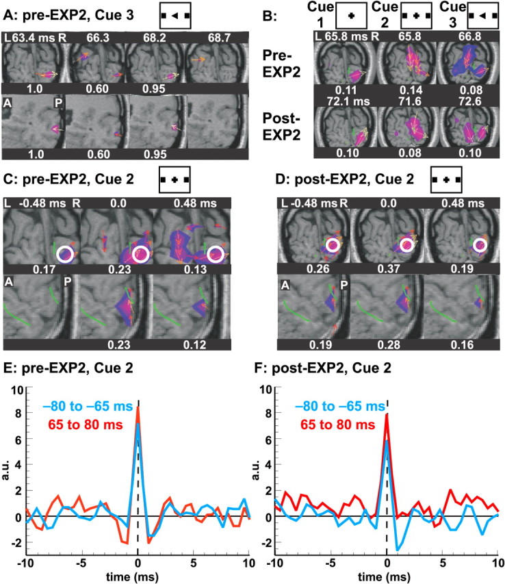
Spikes in V1/V2 during the N70m period, elicited by cue image onset in EXP2 control runs. Each picture is normalized separately, with the maximum for each picture printed as a fraction of the overall maximum. Colors code the modulus of the MFT activity (blue above 0.6 and red above 0.8), and the current density vector above 0.8 of the maximum is shown by the arrows. V1/V2 border is shown as a green outline whenever it is on, or close to, the displayed MRI slice. A, Coronal and right sagittal views of instantaneous MFT single-trial activity (cue 3 in pre-EXP2), showing all recurrences of spikes at two foci close to the calcarine within a 5 ms window. B, Averages aligned to cue onset (cues 1–3) for the pre-EXP2 (top) and post-EXP2 (bottom) run showing N70m maxima for each average. C, D, Averages after alignment of spikes in the latency range of 65–80 ms after cue 2 onset from endogenously generated organization analysis. Alignment was done separately for the pre-EXP2 and post-EXP2 control runs. Separate columns display three successive time slices separated by 0.48 ms, in coronal and sagittal sections through V1, showing the spatial distribution of a spike. The white circles denote V1/V2 ROI. E, F, Realigning to each spike maximum and averaging for the prestimulus period (–85 to –65 ms; blue) and poststimulus period (65–80 ms; red) for the pre-EXP2 (E) and post-EXP2 (F) control runs, showing the brief nature of the spike activity.

The time signature of MEG spikes

Figure 4, E and F, shows the time course for V1/V2 ROI (Fig. 4C,D, white circles) computed with EGO-aligned MFT solutions. Time course reveals a very fast response with amplitude in the center time slice (0 ms) that is approximately twice that of samples on either side (0.48 ms away). These MEG spikes are very likely generated by synchronous spikes because onset, offset, and durations of ∼1 ms cannot be achieved with slow synaptic input. The near constant shape and strength of MEG spikes suggests that very similar population events contribute to each spike. Undershoots, lasting a few milliseconds, are identified in some cases before and/or after the MEG spike peak. This is consistent with what would be expected when probability of the same neuron firing again during the refractory period is reduced. Under this assumption, the strength of undershoot can be interpreted as a measure of the fraction of active neurons captured by the EGO alignment within the corresponding ROI and the period considered.

Separate EGO alignments were made for prestimulus (–80 to –65 ms) and poststimulus (65–80 ms) periods. These time courses are very similar, but close examination reveals subtle differences. For both control runs, the EGO average peak is slightly stronger in the poststimulus (red curves) than the prestimulus (blue curves). A weak undershoot precedes and a stronger one follows the peak in the prestimulus period. For the poststimulus period (Fig. 4E, red curve) that precedes EXP2, the first undershoot is stronger, whereas the second undershoot is almost identical to the corresponding under-shoots for the prestimulus period. These observations suggest that, during pre-EXP2 period, the MEG spikes produced after the visual cue resembled spontaneously occurring spikes in the prestimulus period, with some of the stronger events aligned by EGO preceded by other similar (or weaker) events in some trials. The red curve in Figure 4 F shows no undershoot, suggesting that, in the poststimulus period of post-EXP2, the nonspecific MEG spike background is suppressed, leaving only unitary MEG spikes evoked directly by the visual cue.

MEG spikes in frontal eye fields

Figure 5 shows MEG spikes identified in the frontal eye fields from instantaneous single-trial MFT solutions for type 4 trials (GO/NOGO and movement direction, in one cue) of saccades from center to right. Typical sequences for FEF spikes are shown in Figure 5A for EXP2 (top row) and EXP3 (bottom row), beginning at ∼80 ms before saccade onset. Only time slices with MEG spike activity in either the left or right FEF are displayed, within the continuous latency range of a few milliseconds spanning the MEG spike sequence. For EXP2, the sequence lasts 5 ms (11 time slices), and MEG spike activity is identified in three time slices in the left and two time slices in the right FEF. For EXP3, the sequence lasts 3 ms (seven time slices), and MEG spike activity is identified in three time slices in the left and one time slice in the right FEF. Within a sequence, a spike in either one FEF is identified either singly or in two successive time slices. Sequences for both EXP2 and EXP3 begin and end with weak spikes that bracket a stronger one. Such sequences appear at different times within a trial. Within a sequence, spikes appear at irregular intervals, often in quick succession in the left and right FEF. In each FEF, the current density vector of an MEG spike across trials points in one of two opposite directions. Circular statistical analysis of the data revealed regularities in the seemingly random and intermittent FEF MEG spikes. Figure 5B shows results from circular statistical analysis for type 4 data (GO and movement direction trials analyzing movement to left to right separately) from EXP2 (top) and EXP3 (bottom). For EXP2, the current density direction in each FEF has a bimodal distribution in the 200 ms, leading to left and right saccades with the two peaks at nearly 180° to each other. The distribution becomes nearly unimodal as saccade onset approaches, especially for the FEF contralateral to the saccade direction (marked by a yellow star in the figure). A similar sharpening of a bimodal distribution is also evident for the second subject (EXP3), but this change occurs during saccade onset. For both subjects, the left FEF activity is stronger than that of the right FEF, and the direction for saccades to the contralateral (right) side induces a clear sharpening of the directional distribution. Both subjects were right handed, so these observations are consistent with possible better control of eye movements to the right mediated primarily by the FEF of the dominant (left) hemisphere.

Figure 5.

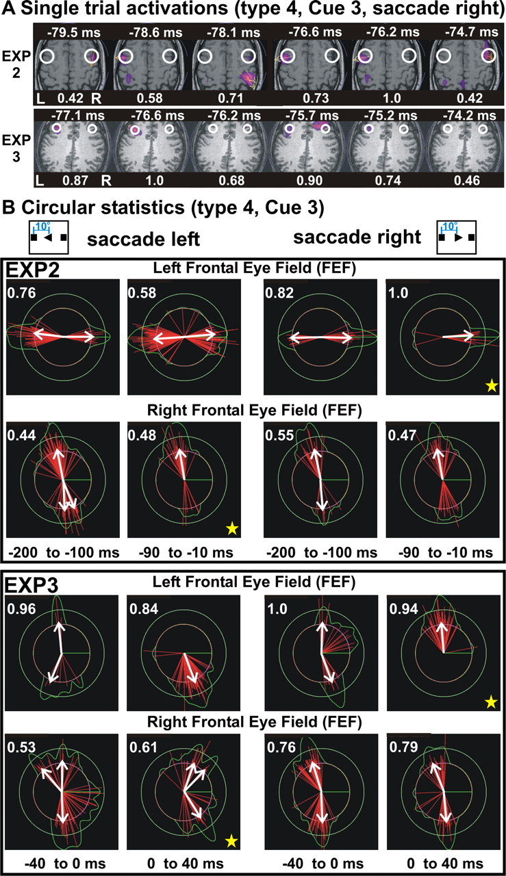
Spike activity in frontal eye fields and a sharpening of current density directions just before or around saccade onset from type 4 runs in EXP2 and EXP3. A, Instantaneous single-trial activations from a saccade from center to right, with FEF ROIs marked by white circles. The top row shows EXP2 in a typical 5 ms window. Spikes from both FEFs are seen. Only on one occasion a spike is captured in two successive time slices (separated by 0.48 ms). The bottom row shows EXP3 in a 3 ms window. Spikes are seen in the left FEF and bilaterally. B, Circular statistics for saccades to the left (left panel) and right (right panel). The white arrow is the significant direction for the vectors as defined by circular statistics. Multiple arrows signify multiple directions. Top, Computed from two presaccadic periods (–200 to –100 ms and –90 to –10 ms) in EXP2. In each FEF, a bimodal distribution is seen, except for the last 90 ms before the saccade, when the distribution is nearly unimodal for the FEF contralateral to the saccade direction of the saccade (marked by yellow stars). Bottom, Computed from around two saccade onset periods (–40 to 0 ms and 0–40 ms) in EXP3. A pattern of activity similar to that for EXP2 is found, especially for saccades to the right.

We next applied circular statistics analysis to MFT solutions after cue 4 of type 2 condition (GO trials, direction information only no movement made). Figure 6 shows that the direction of the current density vector in the left FEF is unimodal for 300 ms beginning 100 ms after the right triangle cue of the GO condition and especially so between 100 and 200 ms after cue 4. The distribution is random for the left-pointing triangle (indicating left saccades in the ipsilateral FEF) or any direction for the NOGO condition [already defined by cue 2 (NOGO)]. For the same cue 4, type 2, the current density direction in the right FEF is bimodal for both right- and left-pointing triangles with a nearly unimodal distribution between 200 and 300 ms after the left-pointing triangle onset. Because cue 4 for type 2 runs provides information about the direction of a saccade to be executed seconds later, the results demonstrate that FEFs do indeed process saccade-related information very soon after the cue becomes available, even when execution of that saccade is not imminent.

Figure 6.

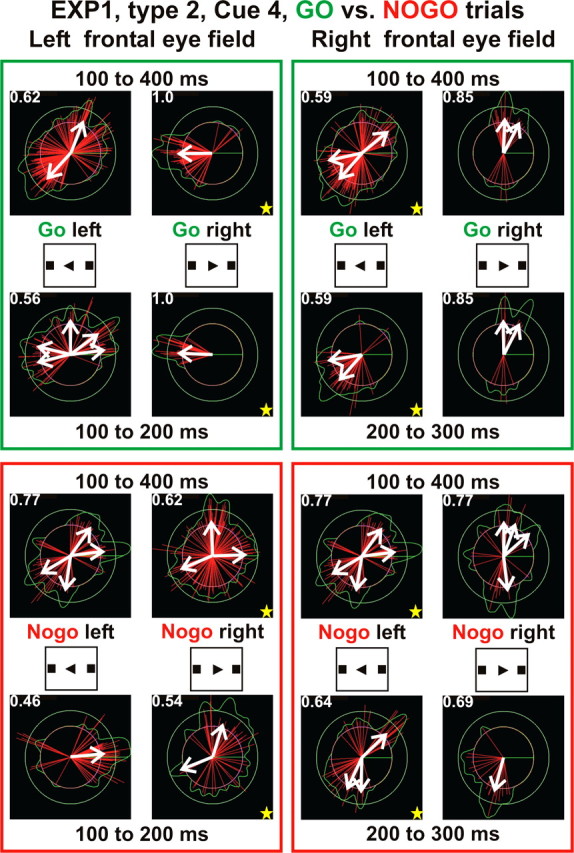
The frontal eye field activity reflects the task demand: circular statistics for frontal eye fields from EXP1, type 2 GO and NOGO trials after cue 4 onset heralding the direction of saccade. The top half (in green boxes) is for GO trials, and the bottom half (in red boxes) is for NOGO trials, and this information is provided 1–3 s before cue 4. The actual saccade for the GO trials is initiated by action cue 6, 1–3 s after cue 4. In each group of pictures, the top row shows the circular statistics for 100–400 ms after the onset of cue 4, and the bottom row shows the circular statistics over a narrower subrange 100 ms long. The yellow stars show the contralateral frontal eye field relative to the saccade direction. The direction of the current density vector becomes more unimodal for contralateral FEF in GO trials but remains random for ipsilateral FEF in GO trials and the NOGO condition.

SPM foci and MEG spikes in cerebellum SPM analysis of EXP2 and EXP3 singletrial MFT solutions for type 3 (movement and direction given in the same cue, all trials GO) and particularly type 4 runs (same as type 3 but with NOGO added) identified the first significant increase in activity in the cerebellum after saccade onset in the left and right flocculi, dorsal vermis, uvula, and nodulus. SPM analysis was performed using 2 and 8 ms windows. Active condition distributions were compared with baseline distributions either from the prestimulus period (–190 to –160 ms) of the same run or from the corresponding pre-EXP2 or pre-EXP3 runs with identical stimuli presented to the subjects. The same foci were identified in the cerebellum with these different SPM computations. Small, well circumscribed SPM foci appeared first in the cerebellum within 25 ms after saccade onset and then spread over the next 50 ms. Inspection of single trials showed that saccade onset was first followed by spikes in either the left or right flocculus or vermis at some time between 15 and 40 ms. These early spikes were followed by persistent activity that often included interchanges of spikes between the flocculi and vermis.

Figure 7 shows cerebellum spike activity and SPM foci on axial MRI cuts at the level of the flocculi and the dorsal vermis. In Figure 7, A and B, white contours show significant early SPM foci, corresponding to p < 0.00001 using an 8 ms window in the SPM comparison between type 4 runs with the appropriate control pre-EXP2 or pre-EXP3 run as baseline. Figure 7A shows also the peaks of instantaneous MFT activity within a 6.8 ms window from a saccade to the right in run 4, type 4, EXP2 (top) and within a 2.4 ms window for saccade to the left in run 6, type 4, EXP3 (bottom). Instantaneous single-trial activations show a very good correspondence with the SPM foci (white contours). Note for EXP2 how, at 17.4 ms, the activity is seen in the left flocculus, then bilaterally at 19.4 ms, and finally in the right flocculus at 24.2 ms. The pattern is similar for EXP3 with the vermis being active at 16.5 ms, then left flocculus at 17 ms, and then bilaterally at 18.9 ms. This rapid interplay between areas is typical in the first few trials of a run in the cerebellum, and it is similar to the rapid interplay between the left and right FEFs observed in the cortex in the presaccadic period (Fig. 6A). Figure 7B shows the first significant SPM foci obtained with the short 2 ms windows for EXP2 and EXP3 type 4 runs. These SPM foci correspond to contrasts between postsaccadic windows and presaccadic (–190 to –160 ms) baseline, and they are displayed on the same axial MRI and with the same white contours as in Figure 7A. The top half of Figure 7B shows the progression of SPM foci for EXP2 for the two runs of type 4, saccades from center to left. The first activation displayed is at 21 ms (green) in the right flocculus and the vermis. It then spreads to left flocculus while remaining in the right at 22 ms (red) and then is seen only in the left flocculus at 23 ms (yellow), having spread in size locally. The dotted green and red contours show the location of the first activation in the next run (run 5), now much more persistent and confined to the left flocculus at 21 ms (dotted green) and continuing with small spreading at 22 ms (dotted red). The bottom half of Figure 7B shows results from EXP3, type 4, run 7 for center to left saccades. For this case, two waves of SPM foci are identified. The first wave begins with bilateral flocculi foci at 30 ms, followed by just the left flocculus at 33 ms. The second wave, at 48 ms, shows SPM foci at both flocculi. Similar interplay between the flocculi and vermis was also seen for center to right saccades (data not shown) for both subjects.

Figure 7.

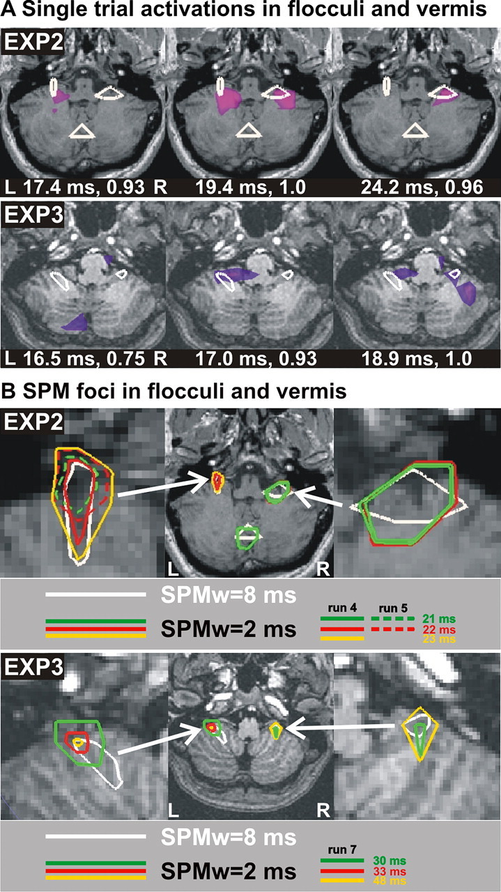
Cerebellum spike activity and SPM foci shown on axial MRI cuts at the level of the flocculi and the dorsal vermis. A, Peaks of activity from a single trial of saccade from center to right. The top half shows peaks of activity for a trial from EXP2, type 4, run 4 at 17.4, 19.4, and 24.2 ms. The MFT result shown in pink/purple is normalized in strength to 1 (middle panel). White contours are early significant SPM foci using an 8 ms window with pre-EXP as baseline. The bottom half shows the same for a trial for saccade to the left from EXP3, type4, run 6 at 16.5, 17, and 18.9 ms. Note that the single-trial activations for both EXP2 and EXP3 show rapid interplay between the flocculi whose positions are in good agreement with both the anatomical definition and the SPM results. B, SPM foci for saccades from center to left in type 4 runs. Top, EXP2, type 4, runs 4 and 5, with a 2 ms window and the presaccadic period (–190 to –160 ms) as baseline. For reference, white contours in A are included. Green centered at 21 ms, red at 22 ms, yellow at 23 ms, all showing precise localization at the flocculi and vermis. Solid color contours are SPM results from run 4, and dotted ones are from run 5, showing rapid habituation of vermis and right flocculi leaving only the ipsilateral (left) floculus SPM focus. Bottom, The same arrangement for EXP3, type 4, run 7, bilateral flocculi are seen active at 30 ms, at 33 ms only in the left flocculus, and at 48 ms in both flocculi again. L, Left; R, right.

Circular statistics analysis of brainstem and cerebellum spikes

Figure 8, A and B, shows the distribution of current density directions for the brain-stem (left and right gaze centers) from EXP2, type 3 runs (all GO with cue 3 giving movement and direction information). Distributions of circular statistics are shown for three intervals: –60 to –20 ms, –20 to 20 ms, and 20–60 ms relative to saccade onset. The figure shows that MEG spikes at 20–60 ms after saccade onset are nearly unidirectional and strongest (relative maxima for the modulus for each circular distribution is the white number at the bottom). Figure 8, C and D, shows the corresponding distributions for gaze center MEG spikes in the same way for EXP3, type 3 runs. The results are very similar to those of EXP2.

Figure 8.

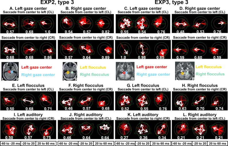
Multiscale bistable intentionality in the gaze centers and flocculi from circular statistics for type 3 runs in EXP2 and EXP3 at three periods, –60 to –20 ms, –20 to 20 ms, and 20–60 ms relative to saccade onset. A–D, EXP2 (A, B) and EXP3 (C, D), left (L) and right (R) gaze center. The top row shows diagrams from saccades from center to left; the bottom row shows diagrams from saccades from center to right. White numbers below each diagram are the largest vector for that picture normalized to the strongest vector in the whole figure for EXP2 or EXP3. EXP2 (E, F) and EXP3 (G, H) left and right flocculi for ipsilateral saccades. For reference, the ROI definitions for the gaze centers and flocculi are also shown on the left and right MRIs, respectively. Note the similarity of pattern across subjects with activity for the time during saccade, becoming focal and unidirectional, with different vector directions for different saccades. Also note the increasing current density as saccade occurs. I–L, Circular statistics diagrams computed for a control area (auditory cortex) in the same hemisphere and periods as the flocculi.

Figure 8, E and F, shows the circular statistics for the flocculi on the ipsilateral side relative to saccades from center to left and right, EXP2 type 3 runs and Figure 8, G and H, for EXP3 type 3 runs. Before the saccade, the distributions for both show no preferred direction. These change, evolving into a bidirectional pattern over saccade onset, except for the left flocculus in EXP3, and then, like the gaze centers, the current flow becomes strong and focal during the saccade. Figure 8I–L shows circular statistics diagrams computed for a control area (auditory cortex) in the same hemisphere and periods as the flocculi. As expected, no obvious organization or modulation is evident across the saccade onset period.

Multiscale bistable intentionality

Circular statistics show preferred direction either after the onset of cues providing directional information or just previous and after saccade onset. During these times, the direction of the current density of MEG spikes in the frontal eye fields, gaze centers, and flocculi changes systematically from a random, to a bimodal, to finally a unimodal distribution. This unimodal distribution is seen for gaze centers just after the saccade is initiated and is probably related to agonist and antagonist neuronal current flow of the ipsilateral and contralateral gaze centers, respectively. The distribution pattern of spikes in the gaze centers before saccades can be interpreted as a measure of planning and preparation. The changes in circular statistics diagrams and their timings for FEFs and the flocculi are also consistent with agonist and antagonist MEG spike activity for the impending saccade. In all cases, the tendency is for a change from either a random or bimodal distribution to a unimodal one. This transition is seen best around saccade onset on the ipsilateral gaze center and flocculus. In the case of the FEFs, the same changes in the circular statistics distribution are better on the contralateral side to the saccade direction. In the FEFs, transitions in circular statistic diagrams are identified as soon as new information about movement direction becomes available, even when the saccade is to be executed a few seconds later (Fig. 6). The clearest transition is evident from the contralateral FEF for the most difficult task (type 4, includes both GO and NOGO) either in the time leading to the saccade (EXP2) or around saccade onset (EXP3). The presence of bimodal distributions over long periods, and across different brain areas when action in one of two possible directions is imminent, implies that plans for both actions are kept in readiness. We call this multiscale bistable intentionality (MBI).

Linked activity between areas in the cortex, cerebellum, and brainstem

We use MI analysis to study how activity in two areas is related. Figure 9 shows results from one subject using data collected at two different sampling rates. In EXP1, the sample rate was 1.6 ms, and the MFT analysis was done for 1 s before and 1 s after cue image onset. The MI analysis was applied with long window length (96 ms) and step (4.8 ms). In EXP2, the sample rate was 0.48 ms, and the MFT analysis was done for 200 ms before to 500 ms after saccade onset, so the MI analysis was applied with short window length (4.8 ms) and step (0.48 ms). The second analysis (for EXP2) was expected to be almost exclusively sensitive to MEG spike activity, whereas the first analysis (for EXP1) was sensitive to activity at lower frequencies. Figure 9A–D shows linked activity over long time scales using the MFT solutions from EXP1 with a window length MI_w = 96 ms and step MI_s = 4.8 ms after establishing a threshold of MI values of 0.8 of the maximum of their respective links. Figure 9, A and B, shows influence diagrams derived from type 2 GO trials aligned to the onset of cue 4. For type 2, cue 4 conveys the saccade direction information, and its onset is 1–3 s after the GO/NOGO cue (cue 2) and 1–3 s before the command to execute the saccade (cue 6). MFT solutions were computed for 1 s before and 1 s after cues 4 and 6 for type 2 trials and showed how V1/V2 activity was linked to other areas throughout the 1 s after cue 4 onset. Figure 9A shows that V1/V2 activity beginning ∼200 ms after the onset of cue 4 is linked to activity in the frontal eye fields ∼400 ms later. Figure 9B shows that V1/V2 activity is linked to gaze center activity soon after cue 4 onset and therefore well before it is linked to the FEFs. Figure 9, C and D, shows interactions between the gaze centers, FEF, and flocculi from type 4 GO trials, with saccade onset alignment. High mutual information was identified that linked activity in the gaze centers to both the cortex and cerebellum. The MI links had long time lags, often lasting for hundreds of milliseconds. The linked activity in the gaze centers began ∼200 ms before saccade onset and continued through the saccade period. Figure 9, E and F, shows MI results for very fast interactions around saccade onset for EXP2 type 4 (MI_w = 4.8 ms; MI_s = 0.48 ms). The links are derived from GO trials aligned to saccade onset and thresholded to MI values higher than mean + 4 SDs of the MI values from the corresponding type 3 trials. Figure 9E shows the interactions between the left (right) gaze center and the flocculi, vermis, and right gaze center. Figure 9F shows the interactions between the right gaze center and the flocculi, vermis, and left gaze center. The strong interplay between the gaze centers and cerebellum around saccade onset during type 4 GO trials is not present in type 3 trials.

Figure 9.

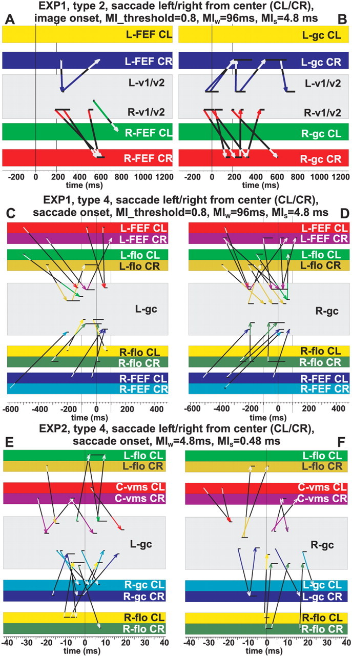
Influence diagrams showing linked activity between areas in the cortex, cerebellum, and brainstem for EXP1 and EXP2. The MI threshold, window length MI_w and step MI_s, are printed above each diagram. A, B, Linked activity between V1/V2 and frontal eye fields (left) and gaze centers (right) from –300 to 1300 ms relative to cue 4 (specifying saccade direction) onset, from type 2 GO trial sin EXP1. C, D, Linked activity between left gaze center and frontal eye field, flocculi (left), and between right gaze center and frontal eye field, flocculi (right) from –600 to 500 ms relative to saccade onset, from type 4 GO trials in EXP1. E, F, Linked activity between left gaze center and flocculi, vermis, right gaze center (left), and between right gaze center and flocculi, vermis, left gaze center from –40 to 40 ms relative to saccade onset, from type 4 GO trials in EXP2. For this diagram, the MI threshold for displaying a link was set to MI values greater than mean + 4 SDs of the MI values from the corresponding type 3 trials.

MI patterns for the second subject (EXP3) were very similar to those of subject one (data not shown). The analysis of type 2 data identified activity in the occipital areas, consistent with V1/V2. This activity was linked to early activity in the gaze centers and then later to FEF. Very fast interactions around saccade onset for EXP3 type 4 were also similar to those of EXP2. Specifically, within the brainstem and cerebellum, the interactions between the two gaze centers and between each gaze center and the flocculi were considerably stronger for type 4 than for type 3 saccades. We computed the link between the gaze centers common to both subjects in EXP2 and EXP3 for type 4 runs with a threshold set at the mean + 4 SDs of the type 3 values. Common links corresponded to increased communication between the gaze centers around saccade onset, as would be expected from the results obtained for each subject separately. The corresponding computation for type 3 produced no common links when the threshold was set to the mean + 4 SDs of the type 4 values. Lowering the threshold to 3 SDs produced only one common strong link. This link was from the right to the left gaze center for saccades to the right beginning 30 ms after saccade onset.

Discussion

Overview of results

We identified intermittent MEG spikes and slower components using a task designed to separate preparation, planning, and execution stages of horizontal saccades. Low-frequency activity dominates the average MEG signal (Figs. 3, 4B); Figure 3A shows a pulse step change of continuous activation in gaze centers leading to constant EOG deflection when the subject fixated on 10° eccentric targets. This concurs with Enderle (2002) and our previous study (Ioannides et al., 2004). Steady level gaze center activity at the end of the traces indicates globe displacement and new position maintenance by balancing ocular muscle tension against those elastic forces pulling the eye back to center (Collins, 1975; Robinson, 1981). Recent neuronal recordings from horizontal gaze centers in cats (Escudero et al., 1992) and primates (McFarland and Fuchs, 1992) support this.

Activation patterns of gaze centers and cerebellum fit with known physiology. Figure 7 shows MEG spikes and the first SPM loci in the vermis and flocculi, after saccade onset. These statistically significant changes in activity are consistent with the roles of these cerebellum structures in controlling initial eye position and monitoring of saccade progress (Enderle, 2002). Each flocculus was more active for ipsilateral saccades, but overall MEG spikes were identified in both flocculi for saccades to the left and right for types 3 and 4 GO trials. The vermis activation was restricted to the dorsal vermis, uvula, and the nodulus (Leigh and Zee, 1999).

The mutual information analysis with long windows (Fig. 9A–D) was sensitive to low-frequency activity and confirmed that saccade-related activity linked areas with long delays lasting for hundreds of milliseconds (Ioannides et al., 2004). These new results show that information about the saccade movement is incorporated into eye movement circuitry as soon as it becomes available even when the saccade is delayed (Fig. 6). The specific links between V1 and brainstem, cerebellum, and frontal eye fields (Fig. 9A,B) support recent claims for saccade-related activity in V1 (Super et al., 2004). The links with long delays between frontal eye fields (Fig. 9C,D) before and after saccade onset are consistent with recent findings in humans that relate FEF activity to postsaccade control of eye fixation (Machado and Rafal, 2004). MI analysis using short windows was dominated by MEG spike activity and showed increased communication between the two gaze centers and the cerebellum when direction information is provided at the same time as GO/NOGO information type 4 trials (Fig. 9E,F).

Properties of MEG spikes and their significance

Processing single-trial MFT solutions found MEG spikes in the same areas that generate low-frequency activity (Figs. 4A,E,F, 5, 6, 7, 8). MEG spikes were intermittent and brief, barely lasting a few milliseconds, and they were present in all examined time periods. The modulation of MEG spikes by visual cues and task differentiated patterns of MEG spikes from ever-present random fluctuations (physiological and/or external noise) in the same frequency range at lower amplitudes. Spike duration and undershoots before and/or after the main peak indicate synchronous action potential activity as candidate generation mechanism, a conjecture supported by both theoretical considerations and experimental evidence. Undershoots would then be consequences of the refractory period of action potentials, and hence the strength of undershoot would be a measure of synchrony. The generation mechanisms of MEG spikes can therefore be discerned from subtle differences in their time courses (Fig. 4E,F). Poststimulus MEG spikes in the post-EXP runs had no under-shoots, and the spatial distribution of the spike-aligned average is sharper and less contaminated by surrounding activity than the corresponding distribution in the pre-EXP period. The spatial specificity of spike-aligned MFT solutions and lack of under-shoots during post-EXP in the poststimulus period suggests that the stimuli-processing threshold increases and thus processing becomes more efficient: when the stimulus arrives in V1, a unitary or small number of synchronous action potential discharges are evoked with minimal background activity.

The detection of MEG spikes supports the synfire chain model hypothesis that implicates a massive synchronous discharge of action potentials (with precise timing of a few milliseconds) through diverging/converging connections in the cortex (Abeles, 1991). The synfire chain model requires that receiving nodes also act as sending nodes in the synfire chain. This idea will be supported if the two opposite current density directions identified in MEG spikes can be shown to correspond to input and output from the same area.

Local connectivity and coupling to the phase of the local field potentials (LFP) is very likely responsible for synchronization of action potentials locally. Recent monkey studies have reported working memory- and attention-related changes in local LFP synchronization in extrastriate visual areas that correlate with bunching of spiking activity. Phase locking of single neuron activity to theta oscillations was identified during short-term maintenance of information (Lee et al., 2005). Attention-related local LFP synchronization (increases in gamma band activity and decreases in lower frequencies) were reported to be correlated with bunching of spiking activity within the 10 ms half-cycle of the gamma band oscillation in V4 (Fries et al., 2001) and more recently to increased efficacy of parallel feature search in the same area (Bichot et al., 2005). Coupling between LFP and single-unit firing probability was also reported in the motor cortex of awake monkeys most prominently in the trained tasks during a pre-movement delay period (Donoghue et al., 1998) and in the middle temporal area (MT or V5) in the period before stimulus presentation in a direction discrimination task (de Oliveira et al., 1997). Modulation of LFP oscillations was also reported in primate cerebellar cortex during active and passive expectancy (Courtemanche et al., 2002). Rapid context-dependent changes have also been reported in the pattern of coincidental action potentials from neurons in the primary cortex of monkeys during a delayed-pointing task (Riehle et al., 1997).

Murthy and Fetz (1996) demonstrated synchronization of 20–40 Hz LFP with submillisecond phase differences over large sensorimotor areas in awake monkeys and illustrated the probability of highest single-unit firing just before the peak of LFP negativity. These diverse observations taken with our identification of MEG spikes across the brain implicates a global mechanism that ensures large-scale coordination. We suggested previously that the global current density generated by rhythmic, persistent activity in deep brain structures such as the hippocampus and nonspecific thalamic nuclei together with impressed currents in cortical areas could serve as a pacing mechanism. Local changes in the intensity and direction of the volume current could recruit and/or coordinate processes going on in parallel across the brain (Ioannides, 1995, 2001). We are now investigating the relationship between MEG spikes and oscillatory activity within and across areas using evoked response paradigms.

Corollary discharges, conjugate, and monocular eye movements

Our results show that saccade preparation and planning can be long and that saccade execution depends on how information is delivered. On saccade initiation, the activity of the gaze center is communicated via corollary discharges to the cerebellum and cortex (Wurtz and Sommer, 2004). Evidence for corollary discharges can also be seen in the frontal eye fields just after saccade onset in the sharp signal-to-noise ratio peaks for the averages aligned with saccade onset in both types 3 and 4 runs in EXP1 (Fig. 3B) and in the mutual information links with long time lag to and from both the cortex and cerebellum beginning 200 ms before saccade onset (Fig. 9C–F).

After saccade initiation, the left and right gaze center SNR time courses are remarkably similar for type 3 averages aligned with saccade onset but not for type 4 averages aligned with cue onset (Fig. 3C). Before saccade initiation, the SNR curves for the two gaze centers for type 4 averages aligned with saccade onset are very similar. These results suggest that conjugate saccades are executed if the GO/NOGO decision is already made but not if it is still pending. In the latter, saccade preparation involves conjugate activity, but monocular corrections are needed during saccade execution. Mutual information results showing a stronger interplay between the gaze centers and cerebellum around saccade onset for type 4 than type 3 runs (Fig. 9E,F) reinforce our interpretations.

Multiscale bistable intentionality

For GO trials, directional information about a future saccade quickly transforms a random distribution of current density into a unidirectional distribution well before any saccade is initiated (Fig. 6). When two saccade directions are possible, regional spikes are often associated with bidirectional current density distributions over long periods, thus keeping both options alive, a state we call MBI. Examples of MBI have been identified for EXP2 and EXP3, types 3 and 4 runs, in the contralateral frontal eye field (Fig. 5B) and ipsilateral gaze centers and flocculi (Fig. 8). MBI requires two simultaneous sustained directional signals corresponding to each of the two possible options, as reported recently for premotor cortex neurons while a primate was choosing between two reaching actions (Cisek and Kalaska, 2005).

In summary, we have identified low-frequency brain activity and MEG spikes that are organized into feedforward and corollary discharges that keep all available options open pending new information.

References

- Abeles M (1991) Corticonics: neural circuits of the cerebral cortex. Cambridge, MA: Cambridge UP.
- Barth DS (2003) Submillisecond synchronization of fast electrical oscillations in neocortex. J Neurosci 23: 2502–2510. [DOI] [PMC free article] [PubMed] [Google Scholar]
- Bichot NP, Rossi AF, Desimone R (2005) Parallel and serial neural mechanisms for visual search in macaque area V4. Science 308: 529–534. [DOI] [PubMed] [Google Scholar]
- Cisek P, Kalaska JF (2005) Neural correlates of reaching decisions in dorsal premotor cortex: specification of multiple direction choices and final selection of action. Neuron 45: 801–814. [DOI] [PubMed] [Google Scholar]
- Collins CC (1975) The human occulomotor control system. In: Basic mechanisms of ocular motility and their clinical implications (Lennerstrand G, Bach-y-Rita P, eds), pp 145–180. Oxford: Pergomon.
- Courtemanche R, Pellerin JP, Lamarre Y (2002) Local field potential oscillations in primate cerebellar cortex: modulation during active and passive expectancy. J Neurophysiol 88: 771–782. [DOI] [PubMed] [Google Scholar]
- Dawson GD (1954) A summation technique for the detection of small evoked potentials. Electroencephalogr Clin Neurophysiol Suppl 6: 65–84. [DOI] [PubMed] [Google Scholar]
- de Oliveira SC, Thiele A, Hoffmann KP (1997) Synchronization of neuronal activity during stimulus expectation in a direction discrimination task. J Neurosci 17: 9248–9260. [DOI] [PMC free article] [PubMed] [Google Scholar]
- Donoghue JP, Sanes JN, Hatsopoulos NG, Gaal G (1998) Neural discharge and local field potential oscillations in primate motor cortex during voluntary movements. J Neurophysiol 79: 159–173. [DOI] [PubMed] [Google Scholar]
- Enderle JD (2002) Neural control of saccades. Prog Brain Res 140: 21–49. [DOI] [PubMed] [Google Scholar]
- Escudero M, de la Cruz RR, Delgado-Garcia JM (1992) A physiological study of vestibular and prepositus hypoglossi neurones projecting to the abducens nucleus in the alert cat. J Physiol (Lond) 458: 539–560. [DOI] [PMC free article] [PubMed] [Google Scholar]
- Fisher NI (1993) Statistical analysis of circular data. Cambridge, MA: Cambridge UP.
- Fries P, Reynolds JH, Rorie AE, Desimone R (2001) Modulation of oscillatory neuronal synchronization by selective visual attention. Science 291: 1560–1563. [DOI] [PubMed] [Google Scholar]
- Hamalainen M, Hari R, Ilmoniemi RJ, Knuutila J, Lounasmaa OV (1993) Magnetoencephalography—theory, instrumentation, and applications to noninvasive studies of the working human brain. Rev Modern Physics 65: 413–497. [Google Scholar]
- Hashimoto I, Kimura T, Tanosaki M, Iguchi Y, Sekihara K (2003) Muscle afferent inputs from the hand activate human cerebellum sequentially through parallel and climbing fiber systems. Clin Neurophysiol 114: 2107–2117. [DOI] [PubMed] [Google Scholar]
- Haueisen J, Schack B, Meier T, Curio G, Okada Y (2001) Multiplicity in the high-frequency signals during the short-latency somatosensory evoked cortical activity in humans. Clin Neurophysiol 112: 1316–1325. [DOI] [PubMed] [Google Scholar]
- Hubener M, Bonhoeffer T (2005) Visual cortex: two-photon excitement. Curr Biol 15: R205–R208. [DOI] [PubMed] [Google Scholar]
- Ikegaya Y, Aaron G, Cossart R, Aronov D, Lampl I, Ferster D, Yuste R (2004) Synfire chains and cortical songs: temporal modules of cortical activity. Science 304: 559–564. [DOI] [PubMed] [Google Scholar]
- Ioannides AA (1995) Estimates of 3D brain activity ms by ms from biomagnetic signals: method (MFT), results and their significance. In: Quantitative and topological EEG and MEG analysis (Eiselt E, Zwiener U, Witte H, eds), pp 59–68. Jena, Germany: Universitatsverlag Druckhaus-Maayer.
- Ioannides AA (2001) Real time human brain function: observations and inferences from single trial analysis of magnetoencephalographic signals. Clin Electroencephalogr 32: 98–111. [DOI] [PubMed] [Google Scholar]
- Ioannides AA, Fenwick PB (2005) Imaging cerebellum activity in real time with magnetoencephalographic data. Prog Brain Res 148: 139–150. [DOI] [PubMed] [Google Scholar]
- Ioannides AA, Bolton JPR, Clarke CJS (1990) Continuous probabilistic solutions to the biomagnetic inverse problem. Inverse Problems 6: 523–542. [Google Scholar]
- Ioannides AA, Liu LC, Kwapien J, Drozdz S, Streit M (2000) Coupling of regional activations in a human brain during an object and face affect recognition task. Hum Brain Mapp 11: 77–92. [DOI] [PMC free article] [PubMed] [Google Scholar]
- Ioannides AA, Corsi-Cabrera M, Fenwick PBC, Portilla YD, Laskaris NA, Khurshudyan A, Theofilou D, Shibata T, Uchida S, Nakabayashi T, Kostopoulos GK (2004) MEG tomography of human cortex and brainstem activity in waking and REM sleep saccades. Cereb Cortex 14: 56–72. [DOI] [PubMed] [Google Scholar]
- Jahn O, Cichocki A, Ioannides AA, Amari S (1999) Identification and elimination of artifacts from MEG signals using extended independent component analysis. In: Recent advances in biomagnetism (Yoshimoto T, Kotani M, Kuriki S, Karibe H, Nakasato N, eds), pp 224–228. Sendai, Japan: Tohoku UP.
- Keller EL (1989) The cerebellum. Rev Oculomot Res 3: 391–411. [PubMed] [Google Scholar]
- Konig P, Engel AK, Singer W (1996) Integrator or coincidence detector? The role of the cortical neuron revisited. Trends Neurosci 19: 130–137. [DOI] [PubMed] [Google Scholar]
- Laskaris NA, Ioannides AA (2001) Exploratory data analysis of evoked response single trials based on minimal spanning tree. Clin Neurophysiol 112: 698–712. [DOI] [PubMed] [Google Scholar]
- Laskaris NA, Liu LC, Ioannides AA (2003) Single-trial variability in early visual neuromagnetic responses: an explorative study based on the regional activation contributing to the N70m peak. NeuroImage 20: 765–783. [DOI] [PubMed] [Google Scholar]
- Lee H, Simpson GV, Logothetis NK, Rainer G (2005) Phase locking of single neuron activity to theta oscillations during working memory in monkey extrastriate visual cortex. Neuron 45: 147–156. [DOI] [PubMed] [Google Scholar]
- Leigh RJ, Zee DS (1999) Synthesis of the command for conjugate eye movements. In: The neurology of eye movements, pp 215–217. New York: Oxford UP.
- Lisberger SG, Pavelko TA, Broussard DM (1994) Neural basis for motor learning in the vestibuloocular reflex of primates. I. Changes in the responses of brain stem neurons. J Neurophysiol 72: 928–953. [DOI] [PubMed] [Google Scholar]
- Liu LC, Ioannides AA (1996) A correlation study of averaged and single trial MEG signals: the average describes multiple histories each in a different set of single trials. Brain Topogr 8: 385–396. [DOI] [PubMed] [Google Scholar]
- Liu LC, Fenwick PB, Laskaris NA, Schellens M, PoghosyaN V, Shibata T, Ioannides AA (2003) The human primary somatosensory cortex response contains components related to stimulus frequency and perception in a frequency discrimination task. Neuroscience 121: 141–154. [DOI] [PubMed] [Google Scholar]
- Machado L, Rafal RD (2004) Control of fixation and saccades during an anti-saccade task: an investigation in humans with chronic lesions of oculomotor cortex. Exp Brain Res 156: 55–63. [DOI] [PubMed] [Google Scholar]
- Makeig S, Westerfield M, Jung TP, Enghoff S, Townsend J, Courchesne E, Sejnowski TJ (2002) Dynamic brain sources of visual evoked responses. Science 295: 690–694. [DOI] [PubMed] [Google Scholar]
- Marsalek P, Koch C, Maunsell J (1997) On the relationship between synaptic input and spike output jitter in individual neurons. Proc Natl Acad Sci USA 94: 735–740. [DOI] [PMC free article] [PubMed] [Google Scholar]
- McFarland JL, Fuchs AF (1992) Discharge patterns in nucleus prepositus hypoglossi and adjacent medial vestibular nucleus during horizontal eye movement in behaving macaques. J Neurophysiol 68: 319–332. [DOI] [PubMed] [Google Scholar]
- Moradi F, Liu LC, Cheng K, Waggoner RA, Tanaka K, Ioannides AA (2003) Consistent and precise localization of brain activity in human primary visual cortex by MEG and fMRI. NeuroImage 18: 595–609. [DOI] [PubMed] [Google Scholar]
- Murakami S, Zhang T, Hirose A, Okada YC (2002) Physiological origins of evoked magnetic fields and extracellular field potentials produced by guinea-pig CA3 hippocampal slices. J Physiol (Lond) 544: 237–251. [DOI] [PMC free article] [PubMed] [Google Scholar]
- Murthy VN, Fetz EE (1996) Synchronization of neurons during local field potential oscillations in sensorimotor cortex of awake monkeys. J Neurophysiol 76: 3968–3982. [DOI] [PubMed] [Google Scholar]
- Ohki K, Chung S, Ch'ng YH, Kara P, Reid RC (2005) Functional imaging with cellular resolution reveals precise micro-architecture in visual cortex. Nature 433: 597–603. [DOI] [PubMed] [Google Scholar]
- Portin K, Vanni S, Virsu V, Hari R (1999) Stronger occipital cortical activation to lower than upper visual field stimuli—neuromagnetic recordings. Exp Brain Res 124: 287–294. [DOI] [PubMed] [Google Scholar]
- Renyi A (1970) Probability theory. Amsterdam: North Holland.
- Riehle A, Grun S, Diesmann M, Aertsen A (1997) Spike synchronization and rate modulation differentially involved in motor cortical function. Science 278: 1950–1953. [DOI] [PubMed] [Google Scholar]
- Robinson DA (1981) Models of the mechanics of eye movements. In: Models of oculomotor behavior and control (Zuber BL, ed), pp 21–41. Boca Raton, FL: CRC.
- Shannon CE (1948) A mathematical theory of communication. Bell Syst Tech J 27: 379–423. [Google Scholar]
- Super H, van der Togt C, Spekreijse H, Lamme VAF (2004) Correspondence of presaccadic activity in the monkey primary visual cortex with saccadic eye movements. Proc Natl Acad Sci USA 101: 3230–3235. [DOI] [PMC free article] [PubMed] [Google Scholar]
- Talairach J, Tournoux P (1988) Co-planar stereotaxic atlas of the human brain. Stuttgart, Germany: Thieme.
- Taylor JG, Ioannides AA, Muller-Gartner HW (1999) Mathematical analysis of lead field expansions. IEEE Trans Med Imaging 18: 151–163. [DOI] [PubMed] [Google Scholar]
- Tesche CD, Karhu J (1997) Somatosensory evoked magnetic fields arising from sources in the human cerebellum. Brain Res 744: 23–31. [DOI] [PubMed] [Google Scholar]
- Tzelepi A, Ioannides AA, PoghosyaN V (2001) Early (N70m) neuromagnetic signal topography and striate and extrastriate generators following pattern onset quadrant stimulation. NeuroImage 13: 702–718. [DOI] [PubMed] [Google Scholar]
- Wurtz RH, Sommer MA (2004) Identifying corollary discharges for movement in the primate brain. Prog Brain Res 144: 47–60. [DOI] [PubMed] [Google Scholar]