Separate Spatial Scales Determine Neural Activity-Dependent Changes in Tissue Oxygen within Central Visual Pathways

Abstract

The relationship between oxygen levels and neural activity in the brain is fundamental to functional neuroimaging techniques. We have examined this relationship on a fine spatial scale in the lateral geniculate nucleus (LGN) and visual cortex of the cat using a microelectrode sensor that provides simultaneous colocalized measurements of oxygen partial pressure in tissue (tissue oxygen) and multiunit neural activity. In previous work with this sensor, we found that changes in tissue oxygen depend strongly on the location and spatial extent of neural activation. Specifically, focal neural activity near the microelectrode elicited decreases in tissue oxygen, whereas spatially extended activation, outside the field of view of our sensor, yielded mainly increases. In the current study, we report an expanded set of measurements to quantify the spatiotemporal relationship between neural responses and changes in tissue oxygen. For the purpose of data analysis, we develop a quantitative model that assumes that changes in tissue oxygen are composed of two response components (one positive and one negative) with magnitudes determined by neural activity on separate spatial scales. Our measurements from visual cortex and the LGN are consistent with this model and suggest that the positive response spreads over a distance of 1–2 mm, whereas the negative component is confined to a few hundred micrometers. These results are directly relevant to the mechanisms that generate functional brain imaging signals and place limits on their spatial properties.

Introduction

Functional neuroimaging techniques are used extensively to study brain function in humans and animals. These techniques infer changes in neural activity from local alterations in brain hemodynamics that are influenced by a combination of vascular and metabolic mechanisms. For example, the blood oxygen level-dependent (BOLD) signal measured with functional magnetic resonance imaging (fMRI) is influenced by changes in cerebral blood flow (CBF), cerebral blood volume (CBV), and the cerebral metabolic rate of oxygen (CMRO₂), each of which is thought to increase during a neural response (Fox and Raichle, 1986; Fox et al., 1988; Belliveau et al., 1991; Mandeville et al., 1998, 1999; Kim et al., 1999). This makes changes in neuroimaging signals difficult to interpret because there are multiple ways in which a given change could arise.

Biophysical models of brain hemodynamics have been developed to improve the interpretability of brain imaging signals (Hathout et al., 1995; Buxton and Frank, 1997; Gjedde, 1997; Buxton et al., 1998; Hyder et al., 1998; Friston et al., 2000; Zheng et al., 2002; Valabregue et al., 2003). These models posit quantitative transformations between a given neural response and a predicted hemodynamic response. They typically define temporal interactions between CBF, CBV, and CMRO₂ but often ignore possible spatial interactions. An implicit assumption is that activity-dependent changes in these variables share similar point spread functions (PSFs) with respect to their influence on the hemodynamic signal. Although this assumption has been examined extensively in recent investigations (Malonek and Grinvald, 1996; Kim et al., 2000; Shtoyerman et al., 2000; Duong et al., 2001; Thompson et al., 2003; Sheth et al., 2004; Thompson et al., 2004; Vanzetta et al., 2004; Devor et al., 2005), there is currently no consensus regarding its validity.

Most studies that examine the spatial specificity of brain imaging signals rely on the columnar organization of primary sensory cortex to control neural responses on a fine spatial scale. However, this approach is limited because subthreshold neural responses are known to spread beyond the borders of activated columns (Grinvald et al., 1994; Das and Gilbert, 1995; Bringuier et al., 1999; Petersen et al., 2003), making the spread of hemodynamic responses difficult to interpret (Devor et al., 2005). Recently, we introduced a microelectrode technique capable of simultaneous, colocalized measurements of tissue oxygen and multiunit neural activity (Thompson et al., 2003, 2004). This technique allows measurements from deep brain structures such as the lateral geniculate nucleus (LGN) in which neural responses can be controlled with greater spatial precision than is possible in the cortex. The LGN is a visual area of the thalamus with precise retinotopic organization and small receptive fields (RFs). Magnification factors in the LGN range between 0.1 and 0.5 mm of tissue per degree of visual angle (Sanderson, 1971). In the current study, we take advantage of these properties of the LGN to vary the pattern of neural activity with respect to our sensor. We use combined oxygen and neural measurements in combination with a simple linear model to quantify the spatiotemporal relationship between neural activity and tissue oxygen. Our results suggest that vascular and metabolic responses to neural activity exhibit similar temporal but substantially different spatial properties.

Parts of this work have been published previously in abbreviated formats (Thompson et al., 2003, 2004).

Materials and Methods

Physiological preparation

All procedures complied with the Society for Neuroscience policy on the use of animals. A total of 14 cats were used in this study. Animals were anesthetized with thiopental sodium (Pentothal) through a venous catheter at a continuous infusion rate determined individually for each animal. Supplementary doses of Pentothal (1–2 mg/kg) were administered as needed during surgery. After a tracheostomy, each animal was placed into a stereotaxic frame and artificially ventilated with 25% O₂ and 75% N₂O at a rate adjusted to maintain expired CO₂ levels between 30 and 40 mmHg (generally 14–22 breaths/min). A craniotomy was performed over each hemisphere at Horsley-Clarke coordinates A6 L9 for LGN recordings and P4 L2 for recordings in visual cortex. After craniotomy, the dura was reflected to expose the cortex. During recording, eye movements were blocked with a continuous intravenous infusion of pancuronium bromide (0.2 mg · kg^–1 · hr^–1). Hydration was maintained by a continuous infusion of lactated Ringer's solution with 2.5% dextrose at a rate of 4 mg · kg^–1 · hr^–1. Drops of 1% atropine sulfate and 2.5% phenylephrine hydrochloride were applied to the eyes to dilate the pupils and retract the nictitating membranes. Rigid contact lenses with 4 mm artificial pupils covered the eyes during recording. Chloramphenicol (50 mg/kg every 12 h) and glycopyrrolate (0.02 mg/kg every 6 h) were administered to prevent infection and inhibit secretions, respectively. After the microelectrode sensor (see below, Dual-purpose microelectrode sensor) was positioned over the target brain location, the craniotomy was sealed with agar and a wax coating. Each animal was positioned in front of a system of mirrors that directs the field of view of each eye to separate halves of a 48.5 × 31 cm cathode ray tube display (Sony, New York, NY). The optical distance from the screen to the animal was 42 cm. The optic disk of each eye was periodically projected onto the visual display with a reversible ophthalmoscope and its position was recorded. We used these measurements to estimate receptive field locations with respect to the area centralis (Vakkur et al., 1963; Nikara et al., 1968; Milleret et al., 1988).

Dual-purpose microelectrode sensor

Recordings were made with a Clark-style polarographic oxygen sensor and an adjacent platinum microelectrode housed within different barrels of a double-barrel micropipette (Unisense, Aarhus, Denmark). The oxygen sensor was polarized with respect to an Ag/AgCl reference electrode (also enclosed within the micropipette) at –0.8 V. This produces an electric current that is linearly related to the partial pressure of oxygen surrounding the sensor tip. Sensors were calibrated in a bath of 0.9% saline at 38°C by bubbling with different mixtures of oxygen and nitrogen. All sensors exhibited linear oxygen calibration curves with sensitivities between 3 and 19 pA/kPa. The 90% response time of the oxygen sensors ranged between 0.9 and 2.5 s, with most sensors close to 1 s. The impedance of the neural electrode was between 0.6 and 2 MΩ depending on the sensor. In total, four different sensors were used for the experiments reported here.

According to the manufacturer, the sensing region of the oxygen sensor is a spherical region with a diameter of ∼60 μm (two times the tip diameter). Therefore, the measured oxygen signal in vivo presumably represents a weighted average of oxygen partial pressure from vascular, extracellular, and intracellular compartments across a small number of capillaries. Here, we refer to this signal as “tissue oxygen” and averaged activity-dependent changes in the signal as “oxygen responses.” Unlike optical imaging and BOLD signals, which are sensitive to the total quantity of deoxyhemoglobin in the vasculature, measurements of tissue oxygen reflect the partial pressure of oxygen within a fixed volume of tissue. This signal is mainly sensitive to alterations in CBF, CMRO₂, and the number of perfused capillaries.

Experimental protocol

The microelectrode sensor was advanced into the LGN or visual cortex (Brodmann's area 17) with a micropositioning motor (EXFO, Mississauga, Ontario, Canada) until visually driven extracellular potentials were identified on the neural electrode. The neural signal was filtered between 0.3 and 10 kHz, and action potentials were discriminated online by setting a threshold ∼2 SDs above the background noise. This signal reflects the collective spike rate of a group of neurons up to a few hundred micrometers from the tip of the sensor. Here we refer to this signal as multiunit neural activity. For recording sites in visual cortex, responses from different single units were initially discriminated based on the shapes of their temporal waveforms but were subsequently summed together during data analysis. All units at a given recording site typically exhibited very similar orientation tuning.

For each recording site, preliminary tests were performed to find the optimal receptive field properties, each defined by the maximum neural spike rate. Recording sites with clear stimulus-induced neural responses [≥10 spikes per second (spk/s) for LGN and ≥5 spk/s for cortex] and small spontaneous oscillations in the baseline oxygen signal were selected for additional study. Approximately 25% of potential recordings sites were passed over because of large baseline oscillations in tissue oxygen. The precise origin of these oscillations is not known, but we presume that they are attributable to alterations in CBF known as vasomotion (Mayhew et al., 1996). Oscillations with similar frequencies (∼0.1 cycles/s) have been observed in CBF and optical imaging measurements within the cerebral cortex (Clark et al., 1958; Mayhew et al., 1996; Kleinfeld et al., 1998; Elwell et al., 1999; Obrig et al., 2000). Oscillations in the LGN are typically higher in frequency and appear to be correlated with the respiration rate of the animal. Oscillations in both brain areas limited the signal-to-noise-ratio (SNR) of the recorded oxygen responses, but we were able to reduce their influence by averaging across multiple trials of the same stimulus condition.

Neural and oxygen signals were measured continuously while different visual stimuli were presented within and around the RF. Visual stimuli were composed of drifting sinusoidal gratings presented monoptically for 4 s on a gray background (50 cd/m²). All stimulus conditions in an experiment were randomly interleaved and repeated between 16 and 80 times depending on the SNR of the oxygen responses. The interstimulus interval was randomized (30–44 s) to avoid possible synchronization with the oscillations described above.

LGN. Oxygen and neural measurements were obtained from a total of 34 LGN recording sites. For each recording site, two experiments were typically performed. The first experiment was performed for all 34 recording sites and consisted of seven or eight stimulus conditions. In four conditions, drifting grating stimuli of various sizes (2°, 5°, 12.7°, and 35°) were positioned over the RF in the dominant eye. In three other conditions, a large-field grating was presented with a mean luminance patch positioned over the RF. The size of this patch was varied (2°, 5°, and 12.7°). The last stimulus condition consisted of a large-field grating presented to the nondominant eye. This stimulus condition was included for only 24 of the 34 recording sites. In all cases, the unstimulated eye viewed a mean luminance gray screen. All gratings were optimized for spatial and temporal frequency and presented with 100% contrast. For 25 of 34 recordings sites, a second experiment was begun immediately after the first. In this experiment, the position of a small (1–2°) grating stimulus was varied with respect to the center of the RF. The position of the stimulus was varied in steps of ∼0.3° to vary the locus of neural activation with respect to the sensor. For both experiments, we remapped the position of the RF every 2 h and adjusted the positions of all stimuli accordingly if any change in position was found. In some cases, the center of the RF moved up to 0.5° during recording attributable to small eye movements or electrode drift.

Visual cortex. Oxygen and neural measurements were obtained from a total of 21 recording sites along the medial bank of the postlateral gyrus (Brodmann's area 17). Optimal stimulus properties (orientation, spatial frequency, position, and size) were identified, and then a single experiment was performed. Between five and six (typically six) different grating orientations were chosen to adequately sample the orientation tuning curve of the recording site. The size of each stimulus was slightly larger than the RF. Orientations included optimal, orthogonal, and additional orientations to sample the sides and the flanks of the orientation tuning curve. Two additional large-field gratings (25°) of optimal orientation were presented to the optimal and non-optimal eye. All gratings were presented with 50% contrast.

Data analysis

Multiunit neural responses are displayed in peristimulus time histograms with bin widths of 133 ms. Low-frequency drift in the oxygen signal was removed by subtracting the baseline signal (average across 10 s period before stimulus onset) from each response before averaging. Oxygen responses were then averaged across identical stimulus conditions and divided by the mean oxygen level for the given recording site. To account for the small delay between actual and measured oxygen changes induced by our sensor, we deconvolved the impulse response function (IRF) of each sensor from each measured oxygen response. Oxygen sensor IRFs were determined by differentiating the response of each sensor to a step change in oxygen concentration. The change in oxygen was induced by quickly transferring the tip of the combined sensor from air to a saline bath of high (>21%) oxygen concentration. Deconvolution was performed in the Fourier domain by dividing each Fourier transformed oxygen response by the Fourier transform of the IRF of the sensor. Before dividing, oxygen responses were low-pass filtered (0.8 Hz cutoff) to remove high-frequency noise that would otherwise be magnified during deconvolution. Finally, the result was inverse Fourier transformed to obtain the adjusted oxygen response. This adjustment has the effect of shifting each oxygen response back in time by ∼0.5 s and increasing its amplitude by ∼7%. Results concerning the spatial properties of the oxygen response are essentially unaffected by this adjustment.

Our analysis of the spatial relationship between neural and oxygen responses requires that we account for neural responses outside of the field of view of the sensor. To do this, we constructed a three-dimensional computer model of the cat's LGN based on published retinotopic maps (Sanderson, 1971). We scanned these maps into digital format and drew a grid on each map using graphics software (Adobe Illustrator; Adobe Systems, San Jose, CA). For each point in the grid, we estimated retinotopic coordinates and anatomical information (layer A, A1, or C) by eye and stored the information in matrix form. Retinotopic points were sampled with a spatial resolution of 0.24 × 0.24 × 0.5 mm and interpolated and smoothed to a resolution of 0.12 × 0.12 × 0.18 mm. We used this model to transform the position of the electrode, RF, and stimulus from visual field coordinates into LGN tissue coordinates. The position of the electrode in this coordinate system is estimated from the dominant eye of the neuron and RF location, which we determined from our neural measurements. The spatial pattern of neural activity, A(r), is then estimated based on the shape of each visual stimulus. We assume a location in the LGN, r′, is active [A(r′) = 1] when its retinotopic coordinates overlap with a high-contrast portion of the visual stimulus. Otherwise, we assume it is inactive [A(r′) = 0]. In this context, “active” means neural activity increases during the stimulus presentation.

Results

Control experiments

To properly interpret measurements obtained with our microelectrode sensor, it is necessary to assess the susceptibility of the oxygen signal to changes in electric potentials. We have done this in two control experiments. In the first experiment, we used a function generator and external electrodes to induce a brief train of electric potentials inside a saline bath. The amplitudes of the electric potentials were more than an order of magnitude greater than those typically observed in vivo. To simulate a neural response, we rapidly increased the frequency of the potentials while recording with the microelectrode sensor. Even with this robust change in frequency, no significant change in the oxygen signal was observed (Fig. 1A).

Figure 1.

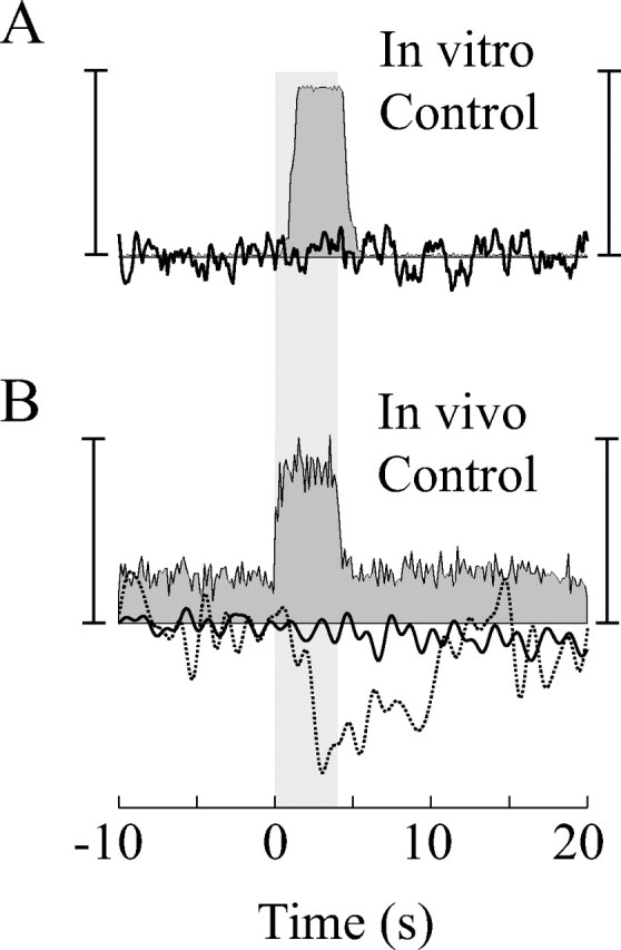
Control data showing no interaction between oxygen and neural electrodes. A, In vitro control performed in 0.9% saline. The bath was bubbled with 5% O₂ and 95% N₂ to establish a baseline oxygen signal (∼40 pA) typical of that observed in vivo. Electric potentials (square wave, +5 V, 0.5 ms duration) were induced with a function generator to simulate neural activity. The frequency of the potentials (gray filled) was increased from 1 to 100 Hz for 4 s. The oxygen signal (black) is unaffected by this change. Displayed responses are averages across eight trials. Vertical scale bars: left, 110 spk/s; right, 1% oxygen change. B, In vivo control performed in the cat's LGN with the oxygen sensor polarization set at 0 V. A small drifting grating stimulus (2°, 100% contrast) was used to elicit neural responses. Neural (grayfilled) and oxygen (black) responses represent averages across eight trials. The dotted line is a normal oxygen response recorded at the same recording site with a normal polarization voltage (–0.8 V). Vertical scale bars: left, 80 spk/s; right, 4% oxygen change. The shaded area in each graph represents the period during which electric potentials are induced.

In a second control experiment, we made in vivo measurements of oxygen and neural signals from the cat's LGN. Robust changes in neural activity were induced with a small drifting grating stimulus (2°) positioned over the RF of the recorded neurons. As expected from previous measurements (Thompson et al., 2004), this stimulus elicited a negative change in the oxygen signal (Fig. 1 B, dotted trace). Next, we removed the polarization voltage of the oxygen sensor. This rendered the sensor insensitive to oxygen without removing it from the circuit. Repeating the same experiment without the polarization voltage abolished the negative oxygen response but left the neural signal unaffected (Fig. 1 B). These control procedures demonstrate that the oxygen signal measured with our sensor is not directly affected by the fast changes in electric potentials induced by active neurons.

Activity-dependent changes in tissue oxygen

LGN

In the first of two experiments, we varied the extent of neural activity generated around the tip of the microelectrode with visual stimuli of different sizes and shapes. We recorded stimulus-induced oxygen and multiunit neural responses from the cat's LGN. Stimulus–response pairs for two example recording sites are shown in Figure 2. For the first four stimulus conditions (Fig. 2A–D), the neural response measured with the microelectrode was relatively constant, although there was a slight reduction for the full-field grating (Fig. 2D) that could be attributable to a suppressive influence of the region surrounding the classical receptive field (Walker et al., 1999; Jones et al., 2000). In contrast, there is a large effect on the time course of tissue oxygen responses and the spatial extent of neural activation as the grating size was changed. The smallest grating stimulus, which elicited a very local increase in neural activity, typically caused a monophasic negative change in tissue oxygen without a substantial positive change (Fig. 2A). The magnitude of this negative response varied across our population, ranging from robust changes detectable on single trials to no detectable change even after averaging over many trials. Examples 1 and 2 of Figure 2 were chosen as representative of the negative response magnitudes we observed. Larger stimuli typically elicited a biphasic oxygen response, consisting of an initial negative change, followed by a later positive response (Fig. 2B–D). However, it was often the case that the delayed positive change was much larger in magnitude than the early negative change, making the negative change difficult to detect in some cases (as in example 2 of Fig. 2).

Figure 2.

Oxygen responses are tuned to the spatial pattern of neural activity in LGN. A–H, Stimulus response pairs for neural and oxygen measurements for two example recording sites in the LGN. The first column depicts the drifting grating stimulus for the dominant and nondominant eyes. The dotted circles inA, F, G, and H represent the location and size of the RF. The second and fourth columns represent a perspective view of a sagittal slice through the left and right LGN, respectively. Simulated patterns of neural activation elicited by the stimulus are depicted in blue/green and are based on the stimulus, RF position, and retinotopic maps of the cat's LGN. Layers A and C (light), layer A1 (dark), and the medial interlaminar nucleus (gray) are represented in each icon. A and M indicate anterior and medial directions, respectively. Horizontal scale bars, 1 mm. The white circle in each icon represents the location of the microelectrode sensor. In the third and fifth columns, each multiunit neural (gray filled) and oxygen (black) response represents an average across 24 and 32 trials, respectively. Dotted lines represent ±1 SEM. Red lines represent fits to the oxygen responses using our model relating the pattern of neural activity to changes in tissue oxygen. Vertical scale bars: example 1, left, 129 spk/s; right, 9% oxygen change; example 2, left, 80 spk/s; right, 16% oxygen change.

The second set of stimulus conditions consisted of a full-field drifting grating and a mean-luminance mask centered over the RF (Fig. 2E–G). These stimuli elicited an increase in neural activity over a large region of the LGN, excluding a volume of tissue surrounding the tip of the microelectrode. The size of the inactive tissue volume was directly related to that of the mask. Because the RF is nearly completely unstimulated, the spike rate measured with the neural electrode was minimal. The smallest mask stimulus elicited a positive change in tissue oxygen without a robust initial negative response. Larger mask stimuli elicited similar time courses but with reduced amplitudes (Fig. 2F,G).

The last stimulus condition (Fig. 2H) consisted of a large-field grating stimulus presented to the nondominant eye. This test was included to elicit a different pattern of neural activity. Because LGN cells are essentially monocular and organized into layers according to eye dominance, this stimulus elicited an increase in neural activity within the layer(s) adjacent to that in which the microelectrode was positioned. Therefore, the neural response near the microelectrode was small or altogether absent. The oxygen response to this stimulus typically exhibited a monophasic positive time course, similar to those elicited by mask stimuli.

The stimulus dependence of the oxygen response depicted in Figure 2 was consistent across our population of LGN recording sites (n = 34). The distribution of positive and negative response magnitudes for each stimulus condition is shown in Figure 3. The dotted line in each panel represents equal positive and negative changes. Notice that most points lie below the dotted line for the small stimulus (Fig. 3A), whereas they all lie above the dotted line for the large-field stimulus (Fig. 3D). Data points cluster along the vertical axis for the small mask stimulus (Fig. 3E), indicating a robust positive response but minimal negative response. The same clustering can be observed in Figure 3H for which robust neural activity was present only in adjacent LGN layers.

Figure 3.

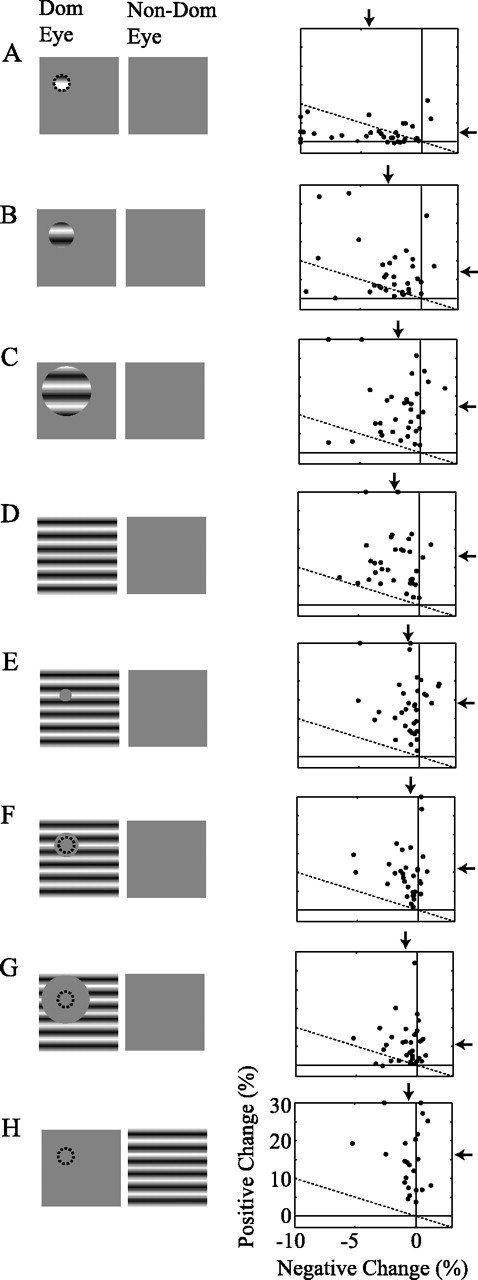
Population data for the first LGN experiment. A–H, Stimulus icons (left) are identical to those in Figure 2. Each scatter plot (right) corresponds to the stimulus condition depicted in the icon to its left and displays the observed oxygen changes across all recording sites. Each point represents the maximum negative (horizontal axis) and positive (vertical axis) change in the average oxygen response for a given recording site. Maximum negative and positive changes are restricted to the first 5 and 10 s after stimulus onset, respectively. Several data points, greater than the limits of the graph (up to –15% for negative changes and 50% for positive changes), have been rescaled to lie on its boarders for display purposes. The dotted line in each plot represents equal positive and negative oxygen changes. Arrows indicate the mean of each distribution.

To examine the spatial specificity of the negative oxygen response, we varied the position of a small visual stimulus with respect to the RF. Figure 4 shows stimulus–response pairs for two example recording sites. As in the first experiment, a small grating stimulus centered over the RF elicited a monophasic negative oxygen response without a subsequent positive component (Fig. 4A). As the stimulus was positioned progressively farther away from the RF center, the locus of activity moved anterior with respect to the electrode (Fig. 4B–F). The magnitude of the negative oxygen response was reduced as the focus of activity moved farther away from the tip of the electrode. This result suggests that the negative oxygen response is well localized to the site of neural activity.

Figure 4.

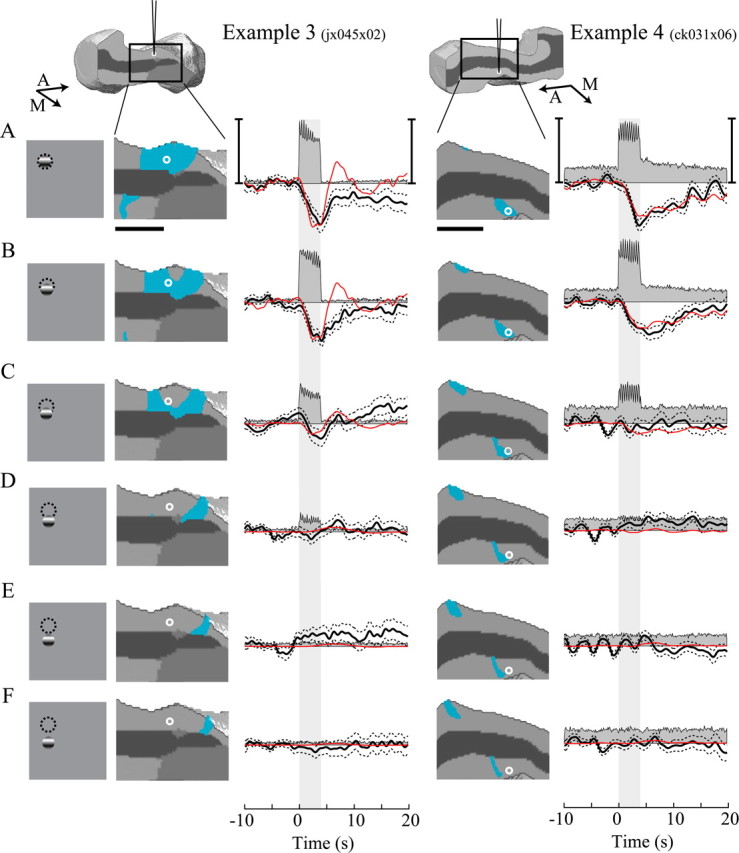
Position of stimulus with respect to the RF affects oxygen and neural responses in the LGN. A–F, Stimulus response pairs for two additional example recording sites. The stimulus icons represent a small drifting grating at varying distances from the center of the RF (dashed circles). The second and fourth columns represent enlarged views of the simulated activity pattern elicited by each stimulus. Horizontal scale bars, 1 mm. The white circle in each icon denotes the estimated location of the microelectrode sensor in the tissue and is based on the position of the RF relative to the area centralis. In the third and fifth columns, multiunit (grayfilled) and oxygen (black) responses represent averages across 56 and 48 trials, respectively. Dotted lines represent ± 1 SEM. Red lines represent fits to each oxygen response using our model relating the pattern of neural activity to changes in tissue oxygen. Vertical scale bars: example 3, left, 60 spk/s; right, 8% oxygen change; example 4, left, 110 spk/s; right, 15% oxygen change. Aa nd M indicate anterior and medial directions, respectively.

This result was also consistent across our population of LGN recording sites. Figure 5 shows population data in the same format as in Figure 3. The maximum negative change (horizontal axis) declines as the stimulus is positioned farther away from the RF. Positive changes in tissue oxygen are small relative to those observed during large-field stimulation. The mean positive change increases slightly as the stimulus moves farther from the RF, but this could be attributable to a small activity-dependent change or a combination of baseline noise and the absence of a strong negative change. Although we show in Figures 2 and 3 that stimuli outside the RF elicit robust positive changes in tissue oxygen, the total volume of neural activity elicited by those large-field stimuli is substantially greater than that caused by the small stimulus in Figures 4 and 5. This is the most likely reason that robust positive oxygen responses were not observed for small stimuli positioned adjacent to the RF.

Figure 5.

Population data for the second LGN experiment. A–F, Stimulus icons (left) are identical to those in Figure 4. Each scatter plot (right) corresponds to the stimulus condition depicted in the icon to its left and displays the observed oxygen changes across all recording sites. Each point represents the maximum negative (horizontal axis) and positive (vertical axis) change in the average oxygen response for a given recording site. Maximum negative and positive changes are restricted to the first 5 and 10 s after stimulus onset, respectively. Several data points, greater than the limits of the graph (up to –19%), have been rescaled to lie on its boarders for display purposes. The dotted line in each plot represents equal positive and negative oxygen changes. Arrows indicate the mean of each distribution.

Visual cortex

The small magnification factors and simple functional organization of the LGN make it ideal for quantifying the spatial properties of the oxygen response, but do other visual areas exhibit similar properties? Although visual cortex has larger magnification factors and more complex functional organization than the LGN, the spatial pattern of neural activity can be changed systematically by taking advantage of the columnar organization of this area. In a previous study, we showed that changes in tissue oxygen could be used to predict the orientation selectivity and ocular dominance of neurons near the microelectrode (Thompson et al., 2003). Here we provide two examples and a population summary of these data (Fig. 6) so that they may be compared with oxygen responses from the LGN.

Figure 6.

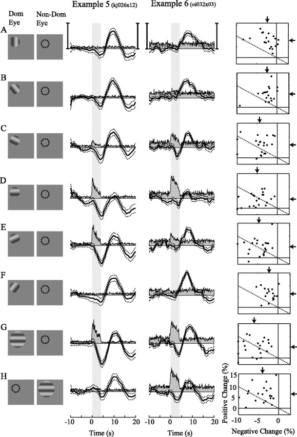
Oxygen responses are tuned to the orientation and ocular dominance of neurons in visual cortex. A–H, Stimulus response pairs for neural and oxygen measurements in the visual cortex. The first column depicts the drifting grating stimulus for the dominant and nondominant eye. The dotted circle represents the location and size of the RF. A–F, Orientation tuning. Six grating orientations were presented. Orthogonal (A) and optimal (D) oriented gratings were interleaved with four additional orientations (B, C, E, F) chosen to coarsely sample the orientation tuning curve of each neuron. G, H, Ocular dominance. Two large-field optimally oriented drifting gratings, one for each eye, were interleaved with the orientation conditions to observe differences attributable to ocular dominance. The second and third columns show multiunit neural (gray filled) and oxygen (black) responses averaged across 80 and 48 trials, respectively. Dotted lines represent ±1 SE of the mean oxygen response. The shaded area represents stimulus onset and duration. Vertical scale bars: example 5, left, 12 spk/s; right, 10% oxygen change; example 6, left, 17 spk/s (left); right, 16% oxygen change. The fourth column shows maximum negative and positive oxygen changes across our population of cortical recording sites (n = 21). Except for the vertical scale, conventions are as in Figures 3 and 5.

In Figure 6, icons on the left represent individual dominant and nondominant eye stimulus conditions used for recording sites in visual cortex (Fig. 6, first column), and graphs to the right show corresponding neural and oxygen responses (Fig. 6, columns 2–4). Note that the actual set of stimulus orientations used for a given recording site is based on the orientation tuning properties of the recorded neurons (see Materials and Methods, Experimental protocol). Figure 6A shows responses to a grating stimulus oriented orthogonal to that preferred by the recorded neuron(s). This stimulus presumably elicits a robust neural response within orientation columns close to, but not overlapping, the tip of our sensor. Although the pattern of neural activity is not identical, the orthogonal stimulus is analogous to the small mask stimulus used in the LGN experiments. Both stimuli elicit neural activity close to, but not overlapping, the recording site. Oxygen responses to these stimuli are also similar. Both elicit a robust positive change in oxygen with a small or absent initial negative change. Figure 6B–F shows oxygen and neural responses for five additional orientation conditions centered on the optimal for a given recording site (Fig. 6D). These stimuli presumably elicit neural activity within orientation columns close to and overlapping the tip of the sensor. The closer the stimulus orientation was to optimal, the larger the initial negative change and the smaller the delayed positive change. This result is consistent with our measurements in the LGN in which neural activity overlapping our sensor typically elicited negative changes in tissue oxygen and activity in surrounding regions elicited slightly delayed positive changes. The last two stimulus conditions show oxygen and neural responses to optimally oriented, large-field stimuli presented to the dominant (Fig. 6G) and nondominant (Fig. 6H) eye. The first example site is strongly monocular. An optimal stimulus in the dominant eye elicits a strong neural response, a robust negative change in tissue oxygen, and a delayed positive oxygen change (Fig. 6G, column 2). The same stimulus presented to the nondominant eye elicited very little neural response close to our sensor but presumably activated neighboring ocular dominance columns several hundred micrometers away. The oxygen response to this stimulus is characterized by a small negative change and a relatively stronger positive change (Fig. 6 H, column 2), similar to nonoptimal orientation conditions. The second example recording site exhibits binocular neural responses (Fig. 6G,H, column 3). The majority of neurons in the cat's visual cortex are binocular such that an optimal stimulus presented to either eye elicits a strong neural response. Oxygen responses in this example exhibit a biphasic response to stimulation of either eye (Fig. 6G,H, column 3). The small difference in response magnitude between right and left eye conditions could be attributable to differences in the pattern of neural activity elicited by the two stimuli. However, in this case, the position of the sensor with respect to the layout of ocular dominance columns is not clear, so the origin of this difference is difficult to determine.

The fourth column of Figure 6 shows positive and negative oxygen response magnitudes for our population of 21 recording sites in visual cortex. The same format is used as in Figures 3 and 5. Oxygen responses across the population are consistent with the two examples shown in Figure 6 and with measurements made in the LGN. The mean negative oxygen response (vertical arrows) is greatest for optimally oriented stimuli presented to the dominant eye, whereas the mean positive oxygen response (horizontal arrows) is largest for non-optimal stimuli and stimuli presented to the nondominant eye.

A model relating neural activity to changes in tissue oxygen

Although our combined oxygen and neural measurements are obtained at a single point in tissue, the results described above suggest that neural responses outside the field of view of the sensor must be considered when interpreting changes in tissue oxygen. We have developed a simple linear model for this purpose. This model relates spatiotemporal patterns of neural activity to activity-dependent changes in tissue oxygen measured with our sensor. For the model, we assume that changes in tissue oxygen are determined by a linear sum of two temporal response components:

(1)

where t is time, r_o is the position of our microelectrode sensor in brain tissue, R is the time course of an oxygen response, and P and N are positive and negative response components, respectively. Note that R represents oxygen changes associated with a given neural response and excludes ongoing changes associated with the baseline state. This two-component model of the oxygen response is motivated by experimental measurements described here and in previous reports (Malonek and Grinvald, 1996; Ances et al., 2001; Masamoto et al., 2003; Thompson et al., 2003, 2004). P and N are determined by convolving the spatiotemporal neural response, A(r,t), with independent spatiotemporal impulse response functions, S_p(r,t) and S_n(r,t):

(2)

(3)

where r is a three-dimensional coordinate in brain tissue and the convolutions are performed in both space and time. One of the primary goals of this study is to quantify the spatial and temporal properties of S_p and S_n. We assume that A, S_p, and S_n are each separable functions with respect to space and time such that

(4)

(5)

(6)

where h_p and h_n are temporal impulse response functions, and w_p and w_n are Gaussian PSFs with independent gain (g_p, g_n) and width (σ_p, σ_n) parameters. σ determines the volume over which neural activity is integrated, and g scales the magnitude of the PSF. The parameters σ_p and σ_n are of particular importance because they determine the spatial specificity between neural and oxygen responses.

Given the assumptions outlined above, the model linking A(r,t) to R(r_o, t) is defined by the following equations:

(7)

(8)

(9)

(10)

(11)

(12)

(13)

(14)

where Equations 8 and 9 are convolutions in space, and Equations 10 and 11 are convolutions in time. The implementation of this model in the context of our LGN measurements is depicted in Figure 7. Our aim is to estimate the parameters g_p, g_n, σ_p, and σ_n. To do this, the model parameters A(r), H_p(t), and H_n(t) must first be specified.

Figure 7.

A model linking the spatial pattern of neural activity to activity-dependent changes in tissue oxygen. For a given visual stimulus, the corresponding pattern of LGN neural activity [A(r)] is convolved with two different Gaussian PSFs, w_p and w_n. r represents a three-imensional coordinate in the LGN. Each PSF corresponds to a different component of the oxygen response and is defined by its width (σ_n and σ_p) and gain (g_n and g_p). The result of each convolution is evaluated at the location of the microelectrode (r_o; white circle) to determine the magnitudes of two temporal response functions, H_n(t) and H_p(t). H_n(t) and H_p(t) are determined empirically at each recording site from responses to small grating and mask stimuli, respectively. Each time course is scaled by its corresponding magnitude [W(r_o)] and summed to determine the predicted oxygen response [R(r_o,t)]. For each recording site, the free parameters σ_n, σ_p, g_n, and g_p are estimated by fitting oxygen responses observed across all stimulus conditions. For the fitting, A(r), H_p(t) and H_n(t) are treated as dependent variables.

We estimated A(r) for each stimulus condition through a combination of our neural measurements and the known retinotopic organization of the cat's LGN (see Materials and Methods). As an example, the estimated pattern of neural activity induced by a large-field drifting grating is shown on the left side of Figure 7. Examples of A(r) for other stimulus conditions are shown in Figures 2 and 4.

We estimated H_n(t) and H_p(t) directly from the oxygen responses elicited by focal and nonfocal LGN activation, respectively. This is possible because the negative and positive response components exhibit substantially different spatial properties such that the relative magnitude of W_p(r_o) and W_n(r_o) in Equations 12 and 13 varies substantially with the spatial pattern of neural activity. In the case of focal activation overlapping the sensor, W_n(r_o) is much greater than W_p(r_o) because the activity pattern fills a greater proportion of the negative component PSF. This, in turn, allows N(t) to dominate the oxygen response. The opposite result occurs during nonfocal activation with mask stimuli. In this case, W_n(r_o) is close to zero, whereas W_p(r_o) is relatively large. By measuring R(r_o, t) in response to these different activity patterns and normalizing the result by its maximum value, the temporal form of H_n(t) and H_p(t) can be estimated. Estimates based on our data are reported below (see Temporal properties). Once A(r), H_p(t), and H_n(t) are specified, the only remaining model parameters are g_p, g_n, σ_p and σ_n. To estimate these parameters, we fit our oxygen measurements with the model by determining values for g_p, g_n, σ_p, and σ_n that minimized the sum-squared error between our data and the fit. For each LGN recording site, all oxygen responses (typically 14) were fit simultaneously with these four free parameters. The fitting algorithm was an interior-reflective Newton method as implemented by the function “lsqcurvefit” in the Optimization Toolbox of Matlab 6.2 (MathWorks, Natick, MA). Fits were performed on the first 10 s of each oxygen response. To test our assumption that the negative and positive response components have different PSF widths, we compared these fits with a second set of fits obtained under the following model constraint: σ_n = σ_p. This constraint forces neural responses to be summed over the same volume of tissue and reduces the number of free parameters from four to three. Results from our data are reported below (see Spatial properties).

In summary, we define a linear model to describe the relationship between neural responses and activity-dependent changes in tissue oxygen. This relationship is characterized by two spatiotemporal impulse response functions. Under a limited number of plausible assumptions, we are able to estimate the shape of these functions from combined measurements of oxygen and neural responses in the cat's LGN. Below, we report estimates of the model parameters derived from our data.

Temporal properties

Consistent with the model described above, results from the LGN and visual cortex suggest that activity-dependent changes in tissue oxygen are composed of two temporal response components, one negative and one positive. Monophasic oxygen responses elicited by focal and nonfocal LGN activation allow us to quantify the temporal properties of these two response components. Specifically, for each LGN recording site, H_p(t) and H_n(t) can be estimated by averaging oxygen responses to mask and small grating stimuli, respectively. To ensure that we obtained the greatest possible dissociation between H_p(t) and H_n(t), only monophasic oxygen responses are included in the average. We define monophasic oxygen responses as those that exhibit a significant (p < 0.001, t test) change in only one direction (positive or negative) within the first 6 s after stimulus onset. After averaging, each time course is normalized by the maximum change in tissue oxygen [maximum negative change for H_n(t)] so that recording sites with large oxygen changes are not over-represented in the population average. We have done this for 26 of 34 LGN recording site in our population. The remaining eight recording sites did not exhibit a monophasic negative change in tissue oxygen, by our definition. For these sites, only H_p(t) could be estimated. Figure 8A shows the population averaged result for both temporal response functions. The negative response [H_n(t); dashed line] begins shortly after stimulus onset, whereas the positive response [H_p(t); solid line] is delayed by ∼1.4 s relative to the negative response. The actual time course for H_n(t) probably makes a smoother transition back to baseline than our estimate suggests. The initially fast return toward baseline that occurs between 6 and 7 s is likely to be the result of a small increase in blood flow that subsides at later time points beyond 10 s.

Figure 8.

Temporal properties of negative and positive oxygen responses. A, Population averaged monophasic negative (dashed) and positive (solid) oxygen responses for our population of LGN recording sites (26 negative and 34 positive responses). The responses shown here represent group estimates for H_p(t) and H_n(t). Times to onset and peak are 0.7 and 3.2 s for the negative response and 2.1 and 5.5 s for the positive response. B, Oxygen responses for optimal (dashed) and orthogonal (solid) orientation conditions averaged across our population of cortical recording sites. Times to onset, dip, and peak are 0.7, 3.3, and 7.6 s for the optimal response and 1.5, 2.8, and 7.4 s for the orthogonal response, respectively. The shaded areas indicate stimulus onset and duration. Times to onset were determined by taking the first time point at which the response magnitude exceeded ±1 SE from baseline. Dotted lines represent ±1SE of the mean response.

Although direct comparison is difficult, we performed a similar analysis for our measurements obtained in visual cortex. Because monophasic negative oxygen responses are rare in visual cortex, probably because of larger RF sizes and magnification factors, we simply averaged oxygen responses to optimal and non-optimal orientation conditions. The population averaged result is shown in Figure 8B. For both optimal (dashed line) and orthogonal (solid line) orientations, time courses exhibit initial negative and delayed positive responses, but the magnitude of the negative response is substantially larger for the optimal stimulus condition. This result is consistent with the data shown in Figure 6. Note that the positive response in visual cortex peaks ∼2 s after that in the LGN. Part of this delay is likely attributable to the negative oxygen response, which has the effect of reducing positive changes during early time points. Other possible sources for this delay include compression of cortical vasculature by our sensor and physiological differences in vascular responsiveness between the LGN and visual cortex.

Spatial properties

Consistent with the model described above, the temporal response components estimated in the previous section [H_p(t) and H_n(t)] appear to have different spatial properties. To quantify the parameters (g_p, g_n, σ_p, and σ_n) that define these spatial properties, we fit our data with the model. Independent fits were performed for each LGN recording site. All oxygen responses recorded at a given site (typically 14) were fit simultaneously with a single set of four free parameters (σ_n, σ_p, g_n, and g_p). The remaining parameters of the model [H_p(t), H_n(t), and A(r)] were specified from our data and from known properties of the cat's LGN. The red time courses in Figures 2 and 4 are fits derived from this analysis. Fits to our data are generally good and account for a large portion of the variance observed across different stimulus conditions. Figure 9A shows the distribution of R² values obtained from our population of LGN recording sites. The mean R² value (arrow) is 0.76 ± 0.13. The fitted parameters σ_n and σ_p determine the width of the PSF for each response component. The full-width at half-maximum (FWHM) of each PSF is calculated from σ using the following equation:

(15)

Histograms of the FWHM values estimated from our analysis are displayed in Figure 9, B and C. We excluded all parameter values obtained from fits with R² < 0.6 (n = 4) and values for g_n and σ_n obtained from recording sites without a significant negative oxygen response (p < 0.001, t test) (n = 8). Figure 9B shows the distribution of widths determined for the negative response component, and Figure 9C shows the distribution for the positive component. In nearly every case, the PSF controlling the negative response is substantially narrower than that of the positive response. Mean width values are 0.15 ± 0.08 and 1.35 ± 0.6 mm for negative and positive PSFs, respectively (means exclude outliers at far right in Fig. 9B,C). An opposite result is exhibited by the PSF gains g_n and g_p. Mean values for g_n and g_p are 1110 ± 1115 and 40 ± 67, respectively. Because the negative PSF sums over a smaller volume of tissue, a larger gain is required for a given change in tissue oxygen. The combination of a narrow PSF width and a large PSF gain leads to the monophasic negative oxygen responses observed during focal activation in the LGN. The large variation in gain values reflects the variation in response magnitude observed across different recording sites (Figs. 3, 5).

Figure 9.

Spatial properties of negative and positive oxygen response components. A, Fit quality (R²) values for our population of LGN recording sites (n = 34). For each recording site, average oxygen responses (1 for each stimulus condition) are fit with the model depicted in Figure 7. Four free parameters (σ_n, σ_p, g_n, and g_p) are used to fit all oxygen responses simultaneously. The dotted line represents a threshold for fit quality. Only parameters derived from fits with an R² value above this threshold are plotted below. B, C, Estimated FWHM values for negative (B) and positive (C) PSFs calculated from σ_n and σ_p using Equation 15 (see Results). Each histogram represents the distribution of parameter values determined from our population of LGN recording sites. Values obtained from recording sites without a significant (p < 0.001, t test) negative change in tissue oxygen are excluded from the histogram in B. Mean values (arrows) are 0.14 ± 0.07 and 1.35 ± 0.6 mm for negative and positive PSFs, respectively. Outliers (bars on far right) are excluded from the population average.

Although the above analysis demonstrates a clear difference between the two estimated width parameters, it could be the case that a model with a single width parameter would fit our data equally well. To test this possibility, we refit our LGN data with the following constraint: σ_n = σ_p. This reduces the number of free parameters to three (σ, g_n, and g_p) and forces neural responses to be summed over the same volume of tissue. Fits using this model are not as good as those obtained with the unconstrained model (mean R² = 0.62 ± 0.26), especially for recording sites at which strong negative responses were elicited. To compare these fits with those from the unconstrained model, we use an F test to account for the slightly different degrees of freedom. Fit quality (sum-squared error) is significantly reduced for 18 of the 34 recording sites under the width constrained model (p < 0.05, F test). The reduction in fit quality is also significant when comparing fits across our entire population simultaneously (F = 12.1, p < 0.0001). Recording sites for which both models yield comparable fits generally have small negative oxygen responses such that the negative response component had little impact over the fit. From this analysis, we conclude that independent PSF widths are necessary to account for our oxygen measurements despite the smaller magnitude of the negative response component.

Discussion

A number of previous studies have reported increases and decreases in tissue oxygen after sensory stimulation of the brain (Meyer et al., 1954; Travis and Clark, 1965; Gijsberg and Melzack, 1967; Sick and Kreisman, 1979; Ances et al., 2001; Masamoto et al., 2003; Thompson et al., 2003, 2004; Offenhauser et al., 2005). In this study, we relate these changes to the spatial pattern of neural activity. We show that focal neural activation elicits monophasic negative changes in tissue oxygen, whereas larger volumes of active tissue cause positive or biphasic responses. Both positive and negative oxygen responses are shown to be localized to the site of neural activity, but the positive response exhibits a considerably wider PSF.

Interpretation of negative and positive changes in tissue oxygen

We interpret the negative component of the oxygen response as arising from local activity-dependent increases in CMRO₂. There is now a general consensus that CMRO₂ increases, at least modestly, during a neural response (Hyder et al., 1996; Hoge et al., 1999; Kim et al., 1999; Vafaee et al., 1999; Mayhew et al., 2000; Kastrup et al., 2002). On its own, this increase in CMRO₂ would cause a negative change in tissue oxygen, but any increase in CBF or the number of perfused capillaries (i.e., capillary recruitment) would act to offset this reduction. We presume that these vascular changes are relatively small during the negative portion of the oxygen response.

To our knowledge, the only alternative interpretation for the negative oxygen response is an activity-dependent reduction in CBF. Although there are recent reports of activity-dependent constriction of blood vessels measured in vitro (Horiuchi et al., 2002; Cauli et al., 2004) and reductions in CBF are thought to underlie sustained negative BOLD responses measured with fMRI (Harel et al., 2002; Shmuel et al., 2002, 2004), these changes are unlikely to be associated with increases in neural activity. In fact, there is evidence that sustained negative BOLD responses are associated with decreases in neural activity (Shmuel et al., 2002, 2004). Furthermore, in vivo studies of activity-dependent CBF changes report that CBF increases during increased neural activity (Leniger-Follert and Lubbers, 1976; Malonek et al., 1997; Kleinfeld et al., 1998; Mathiesen et al., 1998; Jones et al., 2002), even during negative changes in tissue oxygen (Masamoto et al., 2003; Offenhauser et al., 2005). Given that the negative oxygen responses observed in this study were specific to local increases in neural spike rate, it is unlikely that they originated from a reduction in CBF. By similar reasoning, we interpret the positive oxygen response component as arising from activity-dependent increases in CBF. An alternative interpretation is that CMRO₂ is reduced during an increase in neural activity. However, such a change would be contrary to studies showing the opposite result (i.e., CMRO₂ increases with an increase in neural activity) (Hyder et al., 1996; Hoge et al., 1999; Kim et al., 1999; Vafaee et al., 1999; Mayhew et al., 2000; Kastrup et al., 2002).

Hemodynamic point spread function

We have defined a plausible model by which changes in tissue oxygen may be coupled across space with neural activity. A central assumption of the model is that changes in tissue oxygen are composed of two response components (one positive and one negative). Our data suggest that the positive response PSF is substantially wider than that of the negative response. This result accounts for the negative oxygen response observed during focal changes in neural activity (Fig. 2A), as well as the positive oxygen response elicited by spatially extended activation (Fig. 2E). A similar model in which both PSF widths are identical (σ_n = σ_p) does not account for these observations.

Our results are consistent with previous optical imaging and fMRI studies that conclude that the most spatially specific component of the hemodynamic response is related to an early increase in CMRO₂ (Malonek and Grinvald, 1996; Duong et al., 2000; Kim et al., 2000). The conclusion of these previous studies was based on the superior spatial specificity of an early response component, known as the “initial dip,” which is thought to reflect changes in CMRO₂ (Malonek and Grinvald, 1996). Other studies have challenged the interpretation of the initial dip, noting that it could also arise from fast increases in CBV within the venous compartment (Buxton et al., 1998). In addition, it has been suggested that the specificity of the initial dip may be a consequence of the early time at which it is measured rather than the mechanism from which it originates (Sheth et al., 2004). Our current study addresses both of these concerns. Because pure changes in CBV do not alter the oxygen saturation of blood or the partial pressure of oxygen in the tissue, the negative changes in tissue oxygen observed with our sensor cannot be attributed to increases in CBV. Furthermore, our measurements of positive and negative response magnitudes are obtained from identical time points (the first 10 s of each response). Therefore, the difference in specificity we observe between positive and negative response components cannot be attributed to differences in the time at which they are measured. We also find that our results extend to the LGN and are thus not a special property of visual cortex or activation paradigms that rely on columnar organization. However, we cannot rule out the possibility that the initial dip observed with optical imaging and fMRI techniques arises, at least in part, from a different mechanism (e.g., CBV changes).

Models of brain hemodynamics

The model described in this study makes few assumptions regarding the physiological mechanisms that underlie observed changes in tissue oxygen. We have focused mainly on the spatiotemporal properties of the oxygen response rather than on underlying interactions between CBF, CBV, and CMRO₂. Several biophysical models have been proposed that account for these physiological mechanisms (Hathout et al., 1995; Buxton and Frank, 1997; Gjedde, 1997; Buxton et al., 1998; Hyder et al., 1998; Friston et al., 2000; Zheng et al., 2002; Valabregue et al., 2003), but only a few predict activity-dependent changes in tissue oxygen (Gjedde et al., 2002; Zheng et al., 2002; Valabregue et al., 2003) and none consider the spatial pattern of neural activity. Although more complex, models that include tissue oxygen dynamics are able to account for a greater body of experimental data (e.g., hemodynamic changes during hypercapnia) than those that do not. These models also provide a biologically plausible mechanism by which changes in blood flow and oxygen consumption may be uncoupled during neural activity. By this mechanism, a reserve of intracellular oxygen acts as a buffer between oxygen consumption and delivery. Without this reserve, changes in blood flow and oxidative metabolism must be tightly coupled. Our current results support the existence of an oxygen reserve in tissue that may be drawn on in the absence of an increase in blood flow. However, for cases in which the volume of active neurons exceeds a few hundred micrometers, CBF increases more than CMRO₂ and tissue oxygen levels tend to rise rather than fall.

Implications for functional brain imaging

Our results suggest that the ultimate spatial resolution of neuroimaging techniques based on the initial dip may be on the order of a few hundred micrometers, whereas those based on CBF may be limited to a few millimeters. Although accurate localization of activity foci may be possible on finer spatial scales through differential imaging techniques (Frostig et al., 1990) or selective excitation (Sheth et al., 2004), the PSF widths reported here place limits on resolving the underlying pattern of neural activity to a single stimulus condition. It is important to note that our PSF estimates do not account for a number of factors that can significantly degrade spatial resolution. These factors include limitations in imaging hardware, low signal-to-noise ratios, subject motion, and the variability of hemodynamic responses (especially the initial dip). With respect to the initial dip, its specificity is known to degrade within the first few seconds of the response as blood drains from nearby capillaries into relatively distant venules and veins (Duong et al., 2000). Therefore, neuroimaging studies based on the initial dip require simultaneous high spatial and temporal resolution to realize a benefit in spatial specificity. Although this resolution is relatively easy to achieve with optical imaging techniques, it is currently very difficult for fMRI.

To circumvent some of these problems, techniques based on alterations in CBF or CBV may be a more practical alternative for high-resolution neuroimaging (Duong et al., 2001; Sheth et al., 2004). Relative to blood oxygen signals such as the BOLD signal, direct measurements of CBF and CBV are easier to interpret. Changes in CBV are also reported to be larger than changes in blood oxygen and do not drift away from their point of origin (Sheth et al., 2004). One disadvantage is that changes within medium and large blood vessels can lead to substantial vascular artifacts if measures are not taken to reduce their effects (Vanzetta et al., 2004). Data acquisition and post-processing methods have been developed to emphasize the capillary bed component of the CBF and CBV response, which appears to be well localized to underlying neural responses (Frostig et al., 1990; Duong et al., 2001; Sheth et al., 2004; Vanzetta et al., 2004). The width of the positive response PSF estimated in this study is consistent with the finding of well localized CBF and CBV responses because many widths fall below 1 mm (Fig. 9C). However, our data suggest that the specificity of the CBF response is limited in a way that the initial dip is not and that, in some cases, the CBF response may be inadequate for submillimeter spatial resolution.

References

- Ances BM, Buerk DG, Greenberg JH, Detre JA (2001) Temporal dynamics of the partial pressure of brain tissue oxygen during functional forepaw stimulation in rats. Neurosci Lett 306: 106–110. [DOI] [PubMed] [Google Scholar]
- Belliveau JW, Kennedy Jr DN, McKinstry RC, Buchbinder BR, Weisskoff RM, Cohen MS, Vevea JM, Brady TJ, Rosen BR (1991) Functional mapping of the human visual cortex by magnetic resonance imaging. Science 254: 716–719. [DOI] [PubMed] [Google Scholar]
- Bringuier V, Chavane F, Glaeser L, Fregnac Y (1999) Horizontal propagation of visual activity in the synaptic integration field of area 17 neurons. Science 283: 695–699. [DOI] [PubMed] [Google Scholar]
- Buxton RB, Frank LR (1997) A model for the coupling between cerebral blood flow and oxygen metabolism during neural stimulation. J Cereb Blood Flow Metab 17: 64–72. [DOI] [PubMed] [Google Scholar]
- Buxton RB, Wong EC, Frank LR (1998) Dynamics of blood flow and oxygenation changes during brain activation: the balloon model. Magn Reson Med 39: 855–864. [DOI] [PubMed] [Google Scholar]
- Cauli B, Tong XK, Rancillac A, Serluca N, Lambolez B, Rossier J, Hamel E (2004) Cortical GABA interneurons in neurovascular coupling: relays for subcortical vasoactive pathways. J Neurosci 24: 8940–8949. [DOI] [PMC free article] [PubMed] [Google Scholar]
- Clark Jr LC, Misrahy G, Fox RP (1958) Chronically implanted polarographic electrodes. J Appl Physiol 13: 85–91. [DOI] [PubMed] [Google Scholar]
- Das A, Gilbert CD (1995) Long-range horizontal connections and their role in cortical reorganization revealed by optical recording of cat primary visual cortex. Nature 375: 780–784. [DOI] [PubMed] [Google Scholar]
- Devor A, Ulbert I, Dunn AK, Narayanan SN, Jones SR, Andermann ML, Boas DA, Dale AM (2005) Coupling of the cortical hemodynamic response to cortical and thalamic neuronal activity. Proc Natl Acad Sci USA 102: 3822–3827. [DOI] [PMC free article] [PubMed] [Google Scholar]
- Duong TQ, Kim DS, Ugurbil K, Kim SG (2000) Spatiotemporal dynamics of the BOLD fMRI signals: toward mapping submillimeter cortical columns using the early negative response. Magn Reson Med 44: 231–242. [DOI] [PubMed] [Google Scholar]
- Duong TQ, Kim DS, Ugurbil K, Kim SG (2001) Localized cerebral blood flow response at submillimeter columnar resolution. Proc Natl Acad Sci USA 98: 10904–10909. [DOI] [PMC free article] [PubMed] [Google Scholar]
- Elwell CE, Springett R, Hillman E, Delpy DT (1999) Oscillations in cerebral haemodynamics. Implications for functional activation studies. Adv Exp Med Biol 471: 57–65. [PubMed] [Google Scholar]
- Fox PT, Raichle ME (1986) Focal physiological uncoupling of cerebral blood flow and oxidative metabolism during somatosensory stimulation in human subjects. Proc Natl Acad Sci USA 83: 1140–1144. [DOI] [PMC free article] [PubMed] [Google Scholar]
- Fox PT, Raichle ME, Mintun MA, Dence C (1988) Nonoxidative glucose consumption during focal physiologic neural activity. Science 241: 462–464. [DOI] [PubMed] [Google Scholar]
- Friston KJ, Mechelli A, Turner R, Price CJ (2000) Nonlinear responses in fMRI: the Balloon model, Volterra kernels, and other hemodynamics. NeuroImage 12: 466–477. [DOI] [PubMed] [Google Scholar]
- Frostig RD, Lieke EE, Ts'o DY, Grinvald A (1990) Cortical functional architecture and local coupling between neuronal activity and the microcirculation revealed by in vivo high-resolution optical imaging of intrinsic signals. Proc Natl Acad Sci USA 87: 6082–6086. [DOI] [PMC free article] [PubMed] [Google Scholar]
- Gijsberg KJ, Melzack R (1967) Oxygen tension changes evoked in the brain by visual stimulation. Science 156: 1392–1393. [DOI] [PubMed] [Google Scholar]
- Gjedde A (1997) The relation between brain function and cerebral blood flow and metabolism. In: Cerebrovascular disease (Batjer HH, ed), pp 23–40. Philadelphia: Lippincott-Raven.
- Gjedde A, Marrett S, Vafaee M (2002) Oxidative and Nonoxidative metabolism of excited neurons and astrocytes. J Cereb Blood Flow Metab 22: 1–14. [DOI] [PubMed] [Google Scholar]
- Grinvald A, Lieke EE, Frostig RD, Hildesheim R (1994) Cortical point-spread function and long-range lateral interactions revealed by real-time optical imaging of macaque monkey primary visual cortex. J Neurosci 14: 2545–2568. [DOI] [PMC free article] [PubMed] [Google Scholar]
- Harel N, Lee SP, Nagaoka T, Kim DS, Kim SG (2002) Origin of negative blood oxygenation level-dependent fMRI signals. J Cereb Blood Flow Metab 22: 908–917. [DOI] [PubMed] [Google Scholar]
- Hathout GM, Gambhir SS, Gopi RK, Kirlew KA, Choi Y, So G, Gozal D, Harper R, Lufkin RB, Hawkins R (1995) A quantitative physiologic model of blood oxygenation for functional magnetic resonance imaging. Invest Radiol 30: 669–682. [DOI] [PubMed] [Google Scholar]
- Hoge RD, Atkinson J, Gill B, Crelier GR, Marrett S, Pike GB (1999) Linear coupling between cerebral blood flow and oxygen consumption in activated human cortex. Proc Natl Acad Sci USA 96: 9403–9408. [DOI] [PMC free article] [PubMed] [Google Scholar]
- Horiuchi T, Dietrich HH, Hongo K, Dacey Jr RG (2002) Mechanism of extracellular K+-induced local and conducted responses in cerebral penetrating arterioles. Stroke 33: 2692–2699. [DOI] [PubMed] [Google Scholar]
- Hyder F, Chase JR, Behar KL, Mason GF, Siddeek M, Rothman DL, Shulman RG (1996) Increased tricarboxylic acid cycle flux in rat brain during forepaw stimulation detected with 1H[13C]NMR. Proc Natl Acad Sci USA 93: 7612–7617. [DOI] [PMC free article] [PubMed] [Google Scholar]
- Hyder F, Shulman RG, Rothman DL (1998) A model for the regulation of cerebral oxygen delivery. J Appl Physiol 85: 554–564. [DOI] [PubMed] [Google Scholar]
- Jones HE, Andolina IM, Oakely NM, Murphy PC, Sillito AM (2000) Spatial summation in lateral geniculate nucleus and visual cortex. Exp Brain Res 135: 279–284. [DOI] [PubMed] [Google Scholar]
- Jones M, Berwick J, Mayhew J (2002) Changes in blood flow, oxygenation, and volume following extended stimulation of rodent barrel cortex. NeuroImage 15: 474–487. [DOI] [PubMed] [Google Scholar]
- Kastrup A, Kruger G, Neumann-Haefelin T, Glover GH, Moseley ME (2002) Changes of cerebral blood flow, oxygenation, and oxidative metabolism during graded motor activation. NeuroImage 15: 74–82. [DOI] [PubMed] [Google Scholar]
- Kim DS, Duong TQ, Kim SG (2000) High-resolution mapping of isoorientation columns by fMRI. Nat Neurosci 3: 164–169. [DOI] [PubMed] [Google Scholar]
- Kim SG, Rostrup E, Larsson HB, Ogawa S, Paulson OB (1999) Determination of relative CMRO2 from CBF and BOLD changes: significant increase of oxygen consumption rate during visual stimulation. Magn Reson Med 41: 1152–1161. [DOI] [PubMed] [Google Scholar]
- Kleinfeld D, Mitra PP, Helmchen F, Denk W (1998) Fluctuations and stimulus-induced changes in blood flow observed in individual capillaries in layers 2 through 4 of rat neocortex. Proc Natl Acad Sci USA 95: 15741–15746. [DOI] [PMC free article] [PubMed] [Google Scholar]
- Leniger-Follert E, Lubbers DW (1976) Behav of microflow and local PO2 of the brain cortex during and after direct electrical stimulation. A contribution to the problem of metabolic regulation of microcirculation in the brain. Pflügers Arch 366: 39–44. [DOI] [PubMed] [Google Scholar]
- Malonek D, Grinvald A (1996) Interactions between electrical activity and cortical microcirculation revealed by imaging spectroscopy: implications for functional brain mapping. Science 272: 551–554. [DOI] [PubMed] [Google Scholar]
- Malonek D, Dirnagl U, Lindauer U, Yamada K, Kanno I, Grinvald A (1997) Vascular imprints of neuronal activity: relationships between the dynamics of cortical blood flow, oxygenation, and volume changes following sensory stimulation. Proc Natl Acad Sci USA 94: 14826–14831. [DOI] [PMC free article] [PubMed] [Google Scholar]
- Mandeville JB, Marota JJ, Kosofsky BE, Keltner JR, Weissleder R, Rosen BR, Weisskoff RM (1998) Dynamic functional imaging of relative cerebral blood volume during rat forepaw stimulation. Magn Reson Med 39: 615–624. [DOI] [PubMed] [Google Scholar]
- Mandeville JB, Marota JJ, Ayata C, Moskowitz MA, Weisskoff RM, Rosen BR (1999) MRI measurement of the temporal evolution of relative CMRO(2) during rat forepaw stimulation. Magn Reson Med 42: 944–951. [DOI] [PubMed] [Google Scholar]
- Masamoto K, Omura T, Takizawa N, Kobayashi H, Katura T, Maki A, Kawaguchi H, Tanishita K (2003) Biphasic changes in tissue partial pressure of oxygen closely related to localized neural activity in guinea pig auditory cortex. J Cereb Blood Flow Metab 23: 1075–1084. [DOI] [PubMed] [Google Scholar]
- Mathiesen C, Caesar K, Akgoren N, Lauritzen M (1998) Modification of activity-dependent increases of cerebral blood flow by excitatory synaptic activity and spikes in rat cerebellar cortex. J Physiol (Lond) 512: 555–566. [DOI] [PMC free article] [PubMed] [Google Scholar]
- Mayhew J, Johnston D, Berwick J, Jones M, Coffey P, Zheng Y (2000) Spectroscopic analysis of neural activity in brain: increased oxygen consumption following activation of barrel cortex. NeuroImage 12: 664–675. [DOI] [PubMed] [Google Scholar]
- Mayhew JE, Askew S, Zheng Y, Porrill J, Westby GW, Redgrave P, Rector DM, Harper RM (1996) Cerebral vasomotion: a 0.1-Hz oscillation in reflected light imaging of neural activity. NeuroImage 4: 183–193. [DOI] [PubMed] [Google Scholar]
- Meyer JS, Fang HC, Denny-Brown D (1954) Polarographic study of cerebral collateral circulation. Arch Neurol Psychiatry 72: 296–312. [DOI] [PubMed] [Google Scholar]
- Milleret C, Buisseret P, Gary-Bobo E (1988) Area centralis position relative to the optic disc projection in kittens as a function of age. Invest Ophthalmol Vis Sci 29: 1299–1305. [PubMed] [Google Scholar]
- Nikara T, Bishop PO, Pettigrew JD (1968) Analysis of retinal correspondence by studying receptive fields of binocular single units in cat striate cortex. Exp Brain Res 6: 353–372. [DOI] [PubMed] [Google Scholar]
- Obrig H, Neufang M, Wenzel R, Kohl M, Steinbrink J, Einhaupl K, Villringer A (2000) Spontaneous low frequency oscillations of cerebral hemodynamics and metabolism in human adults. NeuroImage 12: 623–639. [DOI] [PubMed] [Google Scholar]
- Offenhauser N, Thomsen K, Caesar K, Lauritzen M (2005) Activity-induced tissue oxygenation changes in rat cerebellar cortex: interplay of postsynaptic activation and blood flow. J Physiol (Lond) 565: 279–294. [DOI] [PMC free article] [PubMed] [Google Scholar]
- Petersen CC, Grinvald A, Sakmann B (2003) Spatiotemporal dynamics of sensory responses in layer 2/3 of rat barrel cortex measured in vivo by voltage-sensitive dye imaging combined with whole-cell voltage recordings and neuron reconstructions. J Neurosci 23: 1298–1309. [DOI] [PMC free article] [PubMed] [Google Scholar]
- Sanderson KJ (1971) The projection of the visual field to the lateral geniculate and medial interlaminar nuclei in the cat. J Comp Neurol 143: 101–108. [DOI] [PubMed] [Google Scholar]
- Sheth SA, Nemoto M, Guiou M, Walker M, Pouratian N, Hageman N, Toga AW (2004) Columnar specificity of microvascular oxygenation and volume responses: implications for functional brain mapping. J Neurosci 24: 634–641. [DOI] [PMC free article] [PubMed] [Google Scholar]
- Shmuel A, Yacoub E, Pfeuffer J, Van de Moortele PF, Adriany G, Hu X, Ugurbil K (2002) Sustained negative BOLD, blood flow and oxygen consumption response and its coupling to the positive response in the human brain. Neuron 36: 1195–1210. [DOI] [PubMed] [Google Scholar]
- Shmuel A, Augath M, Oeltermann A, Pauls J, Logothetis NK (2004) Linking the negative bold response to decreases in neuronal activity in monkey V1. Soc Neurosci Abstr 30: 18.14. [Google Scholar]
- Shtoyerman E, Arieli A, Slovin H, Vanzetta I, Grinvald A (2000) Long-term optical imaging and spectroscopy reveal mechanisms underlying the intrinsic signal and stability of cortical maps in V1 of behaving monkeys. J Neurosci 20: 8111–8121. [DOI] [PMC free article] [PubMed] [Google Scholar]
- Sick TJ, Kreisman NR (1979) Local tissue oxygen tension as an index of changes in oxidative metabolism in the bullfrog optic tectum. Brain Res 169: 575–579. [DOI] [PubMed] [Google Scholar]
- Thompson JK, Peterson MR, Freeman RD (2003) Single-neuron activity and tissue oxygenation in the cerebral cortex. Science 299: 1070–1072. [DOI] [PubMed] [Google Scholar]
- Thompson JK, Peterson MR, Freeman RD (2004) High-resolution neurometabolic coupling revealed by focal activation of visual neurons. Nat Neurosci 7: 919–920. [DOI] [PubMed] [Google Scholar]
- Travis Jr RP, Clark Jr LC (1965) Changes in evoked brain oxygen during sensory stimulation and conditioning. Electroencephalogr Clin Neurophysiol 19: 484–491. [DOI] [PubMed] [Google Scholar]
- Vafaee MS, Meyer E, Marrett S, Paus T, Evans AC, Gjedde A (1999) Frequency-dependent changes in cerebral metabolic rate of oxygen during activation of human visual cortex. J Cereb Blood Flow Metab 19: 272–277. [DOI] [PubMed] [Google Scholar]
- Vakkur GJ, Bishop PO, Kozak W (1963) Visual optics in the cat, including posterior nodal distance and retinal landmarks. Vision Res 61: 289–314. [DOI] [PubMed] [Google Scholar]
- Valabregue R, Aubert A, Burger J, Bittoun J, Costalat R (2003) Relation between cerebral blood flow and metabolism explained by a model of oxygen exchange. J Cereb Blood Flow Metab 23: 536–545. [DOI] [PubMed] [Google Scholar]
- Vanzetta I, Slovin H, Omer DB, Grinvald A (2004) Columnar resolution of blood volume and oximetry functional maps in the behaving monkey; implications for FMRI. Neuron 42: 843–854. [DOI] [PubMed] [Google Scholar]
- Walker GA, Ohzawa I, Freeman RD (1999) Asymmetric suppression outside the classical receptive field of the visual cortex. J Neurosci 19: 10536–10553. [DOI] [PMC free article] [PubMed] [Google Scholar]
- Zheng Y, Martindale J, Johnston D, Jones M, Berwick J, Mayhew J (2002) A model of the hemodynamic response and oxygen delivery to brain. NeuroImage 16: 617–637. [DOI] [PubMed] [Google Scholar]