Angular Path Integration by Moving “Hill of Activity”: A Spiking Neuron Model without Recurrent Excitation of the Head-Direction System

Abstract

During spatial navigation, the head orientation of an animal is encoded internally by neural persistent activity in the head-direction (HD) system. In computational models, such a bell-shaped “hill of activity” is commonly assumed to be generated by recurrent excitation in a continuous attractor network. Recent experimental evidence, however, indicates that HD signal in rodents originates in a reciprocal loop between the lateral mammillary nucleus (LMN) and the dorsal tegmental nucleus (DTN), which is characterized by a paucity of local excitatory axonal collaterals. Moreover, when the animal turns its head to a new direction, the heading information is updated by a time integration of angular head velocity (AHV) signals; the underlying mechanism remains unresolved. To investigate these issues, we built and investigated an LMN-DTN network model that consists of three populations of noisy and spiking neurons coupled by biophysically realistic synapses. We found that a combination of uniform external excitation and recurrent cross-inhibition can give rise to direction-selective persistent activity. The model reproduces the experimentally observed three types of HD tuning curves differentially modulated by AHV and anticipatory firing activity in LMN HD cells. Time integration is assessed by using constant or sinusoidal angular velocity stimuli, as well as naturalistic AHV inputs (from rodent recordings). Furthermore, the internal representation of head direction is shown to be calibrated or reset by strong external cues. We identify microcircuit properties that determine the ability of our model network to subserve time integration function.

Introduction

The rat's limbic system contains head-direction (HD) cells (Ranck, 1984; Taube et al., 1990a) that signal the animal's directional heading. The preferred directions of HD cells distributed uniformly between 0 and 360°. The firing properties are not affected by the animal's spatial location or ongoing behavior and are independent of the local geomagnetic field (Taube et al., 1990b; Goodridge and Taube, 1995; Goodridge et al., 1998; Knierim et al., 1998). HD cells could maintain their directional firing even in darkness (Goodridge et al., 1998). As long as the animal is not disoriented, the preferred direction of an HD cell is well defined according to the relative orientation of the animal with respect to the familiar stable landmarks. The rotation of a salient visual cue in a controlled environment results in an almost equal rotation of the preferred directions of all HD cells (Taube et al., 1990b). These properties endow HD neurons with the functional ability of signaling the rat's sense of direction during spatial navigation.

Head-direction cells have been discovered in several interconnected brain areas in rats (for more details, see Blair and Sharp, 2001; Sharp et al., 2001a; Taube and Bassett, 2003), including the postsubiculum (PoS) (Ranck, 1984; Taube et al., 1990a), the anterior thalamic nucleus (ATN) (Blair and Sharp, 1995; Taube, 1995), the lateral mammillary nucleus (LMN) (Blair and Sharp, 1998; Stackman and Taube, 1998), and the dorsal tegmental nucleus (DTN) of Gudden (Sharp et al., 2001b). This naturally raises the question of which areas are the primary sources of the head-direction signal. Lesions of ATN abolish the directional tuning in the postsubiculum but not the reverse (Goodridge and Taube, 1997). Bilateral, but not unilateral, lesions of the LMN abolish the head-direction signal in the ATN (Tullman and Taube, 1998; Blair et al., 1999). Lesions in the DTN abolish directional firing in the ATN (Bassett and Taube, 2001a). These studies suggest that the head-direction signal may be generated at the level of the LMN-DTN complex. Furthermore, via the nucleus prepositus hypoglossi (nPH), the DTN receives vestibular inputs that carry the angular head velocity (AHV) signal (Lannou et al., 1984; Khalsa et al., 1987), and cells that are tuned to angular head velocity were found in the LMN (Stackman and Taube, 1998) and the DTN (Bassett and Taube, 2001b; Sharp et al., 2001b). Therefore, the LMN-DTN complex is well positioned to integrate the idiothetic (self-motion) signals to produce an internal representation of the head direction.

Several network models have been proposed to explain the mechanism of head-direction signals (Skaggs et al., 1995; Redish et al., 1996; Zhang, 1996; Goodridge and Touretzky, 2000; Rubin et al., 2001; Sharp et al., 2001a; Stringer et al., 2002; Xie et al., 2002). Most models shared similar circuit architecture, in which HD cells are labeled by their preferred directions on a ring and interact with each other through local excitation and lateral inhibition (the “Mexican-hat” connectivity) to produce bell-shaped persistent activity patterns, or “bump attractors.” The direction is thus encoded and maintained by the peak location of a stable persistent activity pattern. This scenario has also been used to model several other neural systems encoding continuous variables (Wang, 2001), e.g., spatial working memory (Camperi and Wang, 1998; Compte et al., 2000; Renart et al., 2003). However, previous models differed in how to integrate self-motion information to update the internal representation (angular path integration). In one approach, an asymmetric component is added to the synaptic connections (Redish et al., 1996; Zhang, 1996), and the strength of the asymmetric component is determined by angular head velocity. This scenario is not biologically plausible because it requires instantaneous change of synaptic connections. In another approach (Skaggs et al., 1995; Zhang, 1996; Goodridge and Touretzky, 2000; Stringer et al., 2002), the network is hardwired and contains “rotation” neurons that receive angular head velocity inputs and, through offset connections to HD cells, are able to move the activity pattern with a speed controlled by AHV. Recently, Xie et al. (2002), following an original suggestion by Zhang (1996), examined this scenario in a “double-ring” model with firing-rate neurons. In particular, the authors showed that the network is able to update HD with a wide range of AHVs.

Previous HD models rely on recurrent excitation. Interestingly, anatomical studies of the LMN-DTN complex (the candidate substrate for HD signal generation) have so far failed to reveal recurrent collaterals in the LMN body (Ramon y Cajal, 1911; Allen and Hopkins, 1988). This raises the conceptual question of whether a continuous attractor network can be realized without recurrent excitation. Moreover, existing models are firing-rate models in which neurons are characterized by spike firing rate and simple network connectivity. To assess the network stability (a major issue for this kind of recurrent circuits) and to help elucidate cellular and circuit mechanisms that underlie neural activity recorded from behaving animals, it is necessary to develop spiking neuron network models in which single cells and synapses are biophysically realistic and microcircuit properties are quantitatively defined. In this paper, we report such a model for the reciprocal loop between excitatory neurons in the LMN (Allen and Hopkins, 1988) and GABAergic inhibitory neurons in the DTN (Allen and Hopkins, 1989). The objectives are twofold. First, we identify microcircuit properties in our LMN-DTN model that are required and sufficient for generating the observed persistent activity and selectivity (tuning) of HD cells. Second, we investigate how such a neural network can serve angular path integration function in the HD system.

Materials and Methods

Network architecture. Our model (Fig. 1) contains one population of excitatory cells (LMN, with N_E = 1024 neurons) and two populations of inhibitory cells (DTN, with N_I1 = 1024 and N_I2 = 1024 neurons, respectively). The choice of N_E = N_I1 = N_I2 is rather arbitrary and is used for the sake of simplicity in computer simulations. The two inhibitory populations form mirror-symmetric images of each other (for details, see below) and play the role of rotation cells as in the model by Skaggs et al. (1995). Neurons in each population are labeled by their preferred directions and distribute uniformly along a ring. For the jth neuron in population α, its preferred direction (in degrees) is θ_j = 360(j/N_α), where α = E, and I₁, I₂ represent the excitatory population, rightward- and leftward-projecting inhibitory populations, respectively. The connection between two neurons (in the same or different populations) depends only on the difference of their preferred directions. In our model, we define the synaptic conductance from cell i of population α to cell j of population β as 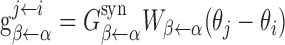, where is the maximal conductance from any neuron in population α to any neuron in population β. The weight function is given by the following expression:

Figure 1.

Network architecture. A, The network consists of three cell populations: one excitatory (square; E) and two inhibitory populations (circle; I₁, rightward-projecting population; I₂, leftward-projecting population). Cells are labeled by their preferred directions. The two inhibitory populations form mirror copies of each other. No recurrent excitation between cells in the E population. Excitatory cells send strongest excitation to neurons with the same preferred direction in I₁ and I₂ populations. Inhibitory cells in the I₁ population send strongest inhibition to excitatory cells on the right side, whereas neurons in the I₂ population send strongest inhibition to excitatory cells on the left side. Connections between inhibitory neurons are not shown. All cells in the E population receive external excitatory inputs (data not shown) simulated as un-correlated Poisson spike trains with fixed rates. Afferent inputs carrying AHV information are modeled as uncorrelated Poisson spike trains to cells in the I₁ and I₂ populations. The rates of the Poisson spike trains are the same for neurons in the same population (b₀ + b₁ for the I₁ population; b₀-b₁ for the I₂ population). The AHV-modulated component b₁ is proportional to the rat's AHV, whereas the AHV-independent component b₀ is the rate when AHV = 0. B, Weight functions of the connections shown in the top. Solid line, I₁→E; dashed line, I₂→E; dotted line, E→I₁ (E→I₂).

where B is the normalization factor determined by . Here, θ₀ is the offset angle (weight function W is maximal when θ = θ₀), and σ is the width (in degrees).

LMN receives inhibitory inputs from DTN (Allen and Hopkins, 1989). In the model, we include connections from the two inhibitory populations to the excitatory population of which the weight functions and are characterized by (Fig. 1). Intuitively, an excitatory cell with preferred direction θ receives strongest inhibition from an I₁ (rightward-projecting) inhibitory cell with preferred direction θ - 110° and an I₂ (leftward-projecting) inhibitory cell with preferred direction θ + 110°. The offset but mirror-symmetric connections from the two inhibitory populations to the excitatory population are critical for angular path integration. No recurrent connections are included between excitatory neurons because of the paucity of recurrent collaterals inside LMN (Ramon y Cajal, 1911; Allen and Hopkins, 1988). To guarantee the discharge of the excitatory neurons, we also include external excitatory inputs modeled as uncorrelated Poisson spike trains of which the rates are the same for all excitatory cells (set to 1800 Hz).

DTN receives excitatory inputs from LMN (Liu et al., 1984; Allen and Hopkins, 1990). We include connections from the excitatory population to the two inhibitory populations, and the corresponding weight functions and are characterized by (Fig. 1). This means that neurons in the two inhibitory populations receive strongest connection from those excitatory neurons with the same preferred direction. Each inhibitory cell population is connected to both itself and to the other inhibitory population. The parameters for the corresponding weight functions are . The two inhibitory populations also receive external excitatory inputs modeled as uncorrelated Poisson spike trains. The rates of the spike trains are modulated by angular head velocity (for details, see below) and are the same for neurons in the same population. Note that these inputs do not represent vestibular input itself (which is an acceleration signal) but afferent to DTN, which envoys information about angular head velocity, because upstream brain regions have already integrated an acceleration signal into a velocity signal (Lannou et al., 1984; Khalsa et al., 1987; McCrea et al., 1999).

Neurons and synapses. Both excitatory and inhibitory neurons are described by a leaky integrate-and-fire (LIF) model (Tuckwell, 1988; Compte et al., 2000; Brunel and Wang, 2001). The time evolution of the membrane potential V_m(t) of a single neuron follows this equation:

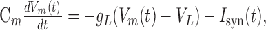where C_m is the membrane capacitance, 0.5 nF for excitatory cells and 0.2 nF for inhibitory cells; g_L is the leak conductance, 0.025 μS for excitatory cells and 0.02 μS for inhibitory cells; and V_L is the resting potential, -70 mV for both excitatory and inhibitory cells. When the membrane potential of a neuron reaches a threshold (-50 mV for both excitatory and inhibitory cells), a spike is fired, and the membrane potential returns to a reset potential (-60 mV for both excitatory and inhibitory cells). Right after a spike, the membrane potential stays at the reset potential for a fixed time period (refractory period, 2 ms for excitatory cells and 1 ms for inhibitory cells).

The last term I_syn(t) in the last equation represents the total synaptic current flowing into the cell. Every neuron receives both recurrent (from neurons in the network) and external synaptic input. In our model, external synaptic inputs are exclusively excitatory and mediated by AMPA receptors. Recurrent synaptic currents include both excitatory (glutamatergic) and inhibitory (GABAergic). The recurrent EPSCs have two components, mediated by AMPA and NMDA receptors, respectively.

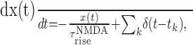
The AMPA-mediated (excitatory) synaptic current (both external and recurrent) is given by I^AMPA = g^AMPAs^AMPA(V_m(t) - V_E), where g^AMPA is the maximal conductance, V_E = 0 mV is the reversal potential of excitatory synapses, and s^AMPA is the gating variable (the fraction of receptors in the open state). The gating variable s^AMPA is described by the following first-order kinetic equation:

where δ(t - t_k) is the Dirac δ function, and t_k is the spike time of the presynaptic (excitatory) neuron. When a spike is fired by presynaptic neuron at time t_k, the gating variable jumps instantaneously by 1; otherwise, it decays exponentially with a time constant of τ^AMPA (set to 2 ms).

Similar to AMPA-mediated synaptic current, the GABA-mediated (inhibitory) synaptic current is given by I^GABA = g^GABAs^GABA(V_m(t) - V_I), where g^GABA is the maximal conductance, V_I = -70 mV is the reversal potential of inhibitory synapses, and s^GABA is the gating variable. The gating variable s^GABA is described by a similar kinetic equation, as follows:

which means that s^GABA decays exponentially with a time constant τ^GABA (we used 10 ms) unless a spike is fired (at time t_k) by the presynaptic neuron (under which s^GABA jumps by 1 instantaneously).

The NMDA-mediated synaptic current is given by the following:

where g^NMDA represents the maximal conductance, V_E = 0 mV is the reversal potential, and s^NMDA is the gating variable. Here,

is the magnesium block (Jahr and Stevens, 1990), where the extracellular magnesium concentration [Mg²⁺] = 1 mm. The gating variable s^NMDA follows kinetic equations (Wang, 1999)

and

where x(t) is an intermediate gating variable, α_NMDA = 1 kHz. When a spike fires at time t_k by the presynaptic neuron, the gating variable s^NMDA increases with a time constant of (set to 2 ms) and then decreases with a time constant of (we used 50 ms). In our simulations, all synapses have a latency of 0.6 ms.

For external AMPA currents, presynaptic spike train is modeled as a Poisson process with a rate ν_ext that is the same for all neurons in each population. The rate for cells in the excitatory population is fixed at 1800 Hz, whereas the rates for cells in the two inhibitory populations are modulated by angular head velocity (for details, see below). The maximal conductance is 0.0057 μS for excitatory cells and 0.0035 μS for inhibitory cells.

As described above, the maximal conductance from cell i of population α to cell j of population β is given by , where is the maximal conductance from any neuron in population α to any neuron in population β, and is the weight function (see above). In most simulations, only NMDA currents were included in the excitatory-to-inhibitory (E-to-I) excitations. The maximal conductances between excitatory neurons were set to . The maximal conductance from excitatory cells to neurons in the two inhibitory populations were set to . For the inhibitory conductance from the two inhibitory populations to cells in the excitatory population, we used and . For the inhibitory conductance between and within each of the two inhibitory populations, we used ,

In some simulations, we introduced AMPA receptor-mediated synaptic transmission. This was done by keeping the total excitatory charge from unitary EPSC at a holding potential of -65 mV fixed. Hence, for 50% AMPA and 50% NMDA contributions, we used For 100% AMPA contribution and no NMDA contribution, we used .

Internal representations of head direction and angular head velocity. Let Θ denote the azimuth angle for the head direction of the animal, then is the AHV, and is the angular acceleration. In a model, let θ be the internal direction represented by the HD cells, and then is the internal representation of AHV. The choice of θ depends on the model details. For example, if a model includes several brain regions (LMN, DTN, ATN, and PoS), one would need to decide which structure most faithfully encodes the animal's HD of the moment. In our model, the peak location of the bell-shaped activity profile of the excitatory population provides a natural choice of the internal representation of the animal's instantaneous head direction. It was determined by a population vector scheme (Georgopoulos et al., 1986), as follows:

where r_i is the firing rate of neuron i, of which the preferred direction is θ_i. When a “hill of activity” moves at a constant propagation speed, the latter was used as a natural internal representation of the animal's AHV.

Angular head velocity signal and landmark inputs. We modeled the angular head velocity signal to the network as uncorrelated Poisson spike trains to neurons in the two inhibitory populations. The rates are modulated by rat's AHV and are the same for neurons in the same population. For simplicity, we denoted the frequency of the spike train to the rightward-projecting inhibitory population b₀ + b₁ and that to the leftward-projecting inhibitory population b₀ - b₁ (Fig. 1). Here, b₀ is the AHV-independent component and equal to the rate when AHV is zero (dΘ/dt = 0). Throughout this paper, we used b₀ = 1800 Hz. The other component b₁ is AHV modulated. The dependence of the afferent input b₁ (to the model network) on the AHV was determined as follows. First, we calculated the dependence of the traveling velocity (denoted by ) of the network activity hill on b₁. This was done by running a set of simulations, each with a different but constant b₁. Let us denote the dependence , where F^-1 is a function. Next, we obtained the dependence of the b₁ on the traveling velocity of the activity hill () by inverting the function F^-1. Finally, because the traveling speed of the activity hill () is the internal representation of the angular head velocity (), it has to be equal to the AHV (). Therefore, the relationship between b₁ and AHV is given by . Given an arbitrary time-varying (t), we used this relationship to obtain b₁(t), which was fed to the network model as the AHV component of the input.

Visual (landmark) inputs are modeled as currents to neurons in the excitatory population, as follows:

where θ_i is the preferred direction of neuron i. The parameter A > 0 determines the strength of visual inputs, θ₀ is the allocentric bearing of the landmark (neurons with preferred direction θ₀ receive strongest visual input), and σ is the width (range) of the visual input.

Directional tuning curve. The directional tuning curve of a single neuron (firing rate f vs head direction θ) has been fitted by the following function (Zhang, 1996):

where θ₀ is the preferred direction of this neuron, and A, B, and K are positive parameters. The maximal firing rate is A + Be^K, and the directional firing range (base width) is defined as 230°/K. The nonlinear curve fitting was done by using a Levenberg-Marquardt algorithm.

Integrating experimental angular head velocity data. To test whether our model network could integrate real-time angular head velocity data accurately, head-direction data recorded from freely moving rats (courtesy of J. Taube, Dartmouth College, Hanover, NH) were used. The HD time series was sampled at 60 Hz, so the time bin is ∼16.7 ms. First, we smoothed the head-direction data by averaging over five data points centered at the middle time. Next, we estimated the rat's AHV for each time period of 16.7 ms as the change in head direction divided by the time bin size (16.7 ms), which yielded a time-varying . We then used the relationship (described above) to obtain the AHV component of the input to the model network, b₁ to the rightward-projecting inhibitory population and -b₁ to the leftward-projecting population. The integration performance of the model network was evaluated by comparing the peak location of the activity hill with the experimental HD time series and quantified by the cumulative error (difference between the two) over time.

Numerical methods. The integration method we used for the differential equations was a second-order Runge-Kutta algorithm with an interpolation scheme for the firing time (Hansel et al., 1998; Shelley and Tao, 2001). The time step we used was 0.02 ms. We also used a fast Fourier transform program FFTW (Frigo and Johnson, 1998) for the efficient calculation of synaptic inputs. Random numbers used in the simulation were generated by RngStream (L'ecuyer et al., 2002). All of the code was written in C++ and compiled with g++3.3 (GNU C++).

Results

Stationary hill of persistent activity

We first consider the behavior of our model in the absence of sensory and/or self-motion signals. This corresponds to the case in which animal's head direction is held fixed. In our model, it is implemented by setting to zero (b₁ = 0) the AHV component of the external afferent inputs to the two inhibitory populations (see Materials and Methods). In this case, the network quickly (in <100 ms) settles into a stationary state with a bell-shaped activity profile (Fig. 2B). Because of the symmetries of the network (Fig. 1), the peak of the activity hill can be anywhere in the network (depending on the initial condition); thus, the system can represent any head direction as an analog quantity.

Figure 2.

Self-sustained persistent activity without recurrent excitation. A stationary hill of activity emerges when the AHV-modulated component of the afferent input is zero (b₁ = 0). The peak of the hill of activity is equally likely to appear at any direction (the peak is ∼180° for the example shown here). A, Traces of the membrane potential of three cells from the excitatory population, with preferred directions 134°, 180°, and 227°, respectively. B, Left, Rastergram of the excitatory population (top) and two inhibitory populations (middle and bottom). Abscissa, Time; ordinate, neurons labeled by their preferred directions. Each dot represents a spike. The thick black line in the top plot is the center of the activity profile calculated by the population vector method. Right, Bell-shaped network activity profiles average over a time period of 6 s. C, Synaptic current distribution across three cell populations. From left to right, Synaptic current profiles for the E, I₁, and I₂ populations, respectively. Red, External current; magenta, recurrent NMDA current; green and blue, recurrent inhibitory currents from the I₁ and I₂ populations; black, total current. All currents, including external, recurrent excitatory, and total inhibitory currents (sum of the inhibitory currents from the I₁ and I₂ populations), are symmetric with respect to the center of the hill of activity, which is ∼180°. I_n (C) - I_syn is plotted.

As mentioned in Introduction, there is no synaptic connection between cells in the excitatory population. The hill of activity is generated and maintained by a combination of uniform external excitatory input and structured inhibitory inputs from the two inhibitory populations. This is shown in Figure 2C, in which synaptic currents of different sources in single cells are plotted across the network. The distribution of the external excitation is uniform (red), whereas the distributions of the inhibitory currents from the two inhibitory populations (blue and green) are symmetric with respect to the center of the activity hill (∼180°). As a result, the profile of the total synaptic current has a Mexican-hat shape (black) and is symmetric with respect to the center of the activity hill.

Traveling hill of activity with constant velocity

When the angular head velocity, hence the AHV component of the afferent input (b₁), is non-zero but constant, the activity hill no longer stays stationary but travels with a constant velocity (Fig. 3B, in which b₁ = -200 Hz, and the traveling velocity of the activity hill is ∼489°/s). Intuitively, this result (Fig. 3) can be explained as follows. Because of a stronger external drive (b₀ - b₁ = 2000 Hz vs b₀ + b₁ = 1600 Hz), neurons in the leftward-projecting inhibitory population (Fig. 3B, bottom) discharge at higher rates than their counterparts in the rightward-projecting inhibitory population (Fig. 3B, middle). This imbalance of firing results in stronger inhibitions to neurons on the left side of the excitatory activity hill than to their counterparts on the right side (Fig. 3C, left column, blue vs green) and causes the hill of activity to travel rightward.

Figure 3.

Moving hill of activity. The spatially tuned firing pattern propagates at a constant speed when afferent input is non-zero but constant (b₁ = -200 Hz). A, Membrane potential trace of three cells from the excitatory population, with preferred directions 90°, 180°, and 270° respectively. B, Rastergram of the excitatory population (top) and two inhibitory populations (middle and bottom). Abscissa, Time; ordinate, neurons labeled by preferred direction. Each dot represents a spike. The thick black line in the top plot is the peak of the activity profile calculated by population vector method, which is used as the internal representation of the head direction. The peak of the hill of activity is moving with a constant speed of ∼489°/s. C, Network synaptic current profiles of the moving hill of activity. From left to right, Profiles for the E, I₁, and I₂ populations. Red, External current; magenta, recurrent NMDA current; green and blue, recurrent inhibitory current from the I₁ and I₂ populations; black, total current. All of the synaptic currents are calculated at time t = 750 ms (dotted line in top plot of B), when the peaks of the hill of activity are ∼180°. For excitatory cells, the synaptic current profiles from the two inhibitory populations (green vs blue) are asymmetric with respect to the peak of the hill of activity, as is the total current. I_n (C) - I_syn is plotted.

Figure 4 shows the dependence of the traveling velocity of the activity hill on the afferent input b₁. Each data point was obtained from a simulation with a constant b₁, which resulted in a moving activity hill at constant velocity. The traveling velocity of the activity hill depends on b₁ linearly with a slope of -2511° · s^-1 · kHz^-1 when|b₁| ≤ 0.4 kHz. It saturates to a speed of ∼1670°/s when|b₁| ≥ 0.7 kHz. We denote the inverse of this relationship as b₁ = F(AHV), which can be used to convert an AHV value to the corresponding input to the network b₁ (see Materials and Methods). Therefore, the model network is able to integrate over a wide range of AHVs, including those expected for a rodent HD system (for an example, see Fig. 10A).

Figure 4.

Traveling velocity of the hill of activity is proportional to the afferent input b₁, in a wide range of moving speeds. Ordinate, Moving speed of the activity hill; abscissa, AHV-modulated afferent input b₁. The speed of the activity hill is measured by the speed of the peak of the excitatory activity hill, which is estimated by a population vector method. The afferent inputs to the two inhibitory populations (rates of the external Poisson spike trains) are b₀ + b₁ and b₀ - b₁, respectively (see also Fig. 1). Here, b₀ is the AHV-independent component (set to 1800 Hz), and b₁ is the AHV-modulated component. When b₁ = 0, the hill of activity is stationary (speed is 0; see Fig. 2). When|b₁| ≤ 0.4, the traveling velocity depends on b₁ approximately linearly (with a slope of approximately -2511° · s^-1 · kHz^-1). When|b₁| ≥ 0.7, the speed saturates (with a maximal speed of ∼1670°/s).

Figure 10.

Integration of the angular head velocity profile recorded from a freely moving rat (data provided by J. Taube). A, Experimental AHV profile to be integrated by the model network (left) and its histogram (right). B, The model network integrates the naturalistic AHV profile fairly well. Thick gray line, Experimental HD profile; black lines, traces of the excitatory activity hill in 20 trials. Abscissa, Time; ordinate, head direction. C, Left, Time evolution of the integration error in 20 trials (black lines) and their mean (gray line). Right, The variance of the integration error across 20 simulations increases with time.

HD tuning curves and their AHV modulation

The firing properties of HD cells are characterized by their tuning curves (firing rate vs HD). The tuning curves are often quantified by a Gaussian function or a triangular function. In either case, they are characterized by three parameters: the cell's preferred firing direction, peak firing rate, and firing range (Taube et al., 1990a; Taube, 1995; Stackman and Taube, 1998). In this section, we compare quantitatively the tuning curves of our model neurons with available experimental data. For LMN HD cells (excitatory cells in our model), Stackman and Taube (1998) reported that the peak firing rate (n = 20) was 69.53 ± 13.67 Hz, ranging from 9.75 to 226.46 Hz. On the other hand, Blair and Sharp (1998) reported that the peak firing rate (n = 23) was 37.2 ± 5.5 Hz. Our simulation result (Fig. 5B, left column) is in the range of Stackman and Taube (1998). Stackman and Taube (1998) also reported that the directional firing range (defined as the width of the tuning curve at background firing rate) was 168.16 ± 8.04°, ranging from 81.01 to 220.07°. Blair and Sharp (1998) reported that the tuning width (defined as twice the SD of the directional tuning function) was 79.9 ± 3.5°. The firing range of the tuning curve of the excitatory cell in our simulation (Fig. 5C, left column) is in the range of Stackman and Taube (1998).

Figure 5.

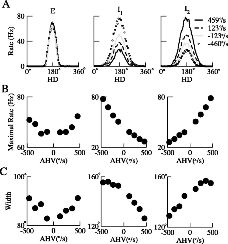
Angular head velocity modulation of the head-direction tuning curves. From left to right, neurons are chosen from the E, I₁, and I₂ populations, respectively. A, Head-direction tuning curves under different angular head velocity. Each curve was obtained from simulation with fixed afferent input b₁. B, The peak firing rate as a function of angular head velocity. The cell from the excitatory population shows symmetric AHV modulation, whereas the two cells from the two inhibitory populations show asymmetric angular head velocity modulation. Cells from the two inhibitory populations behave in the opposite way: one prefers clockwise turning, whereas the other prefers counterclockwise turning. Note that the velocity sensitivity of the inhibitory neurons (middle and right columns) is approximately three times of that of the excitatory neurons (left column). All three types of AHV modulation of HD tuning curves have been observed experimentally. C, The width of the tuning curves as a function of angular head velocity. For the excitatory cell (left), the width increases when the amplitude of the AHV increases. For inhibitory cells, the width increases when AHV increases on one direction but decreases on the other. Neurons from different inhibitory populations (middle vs right columns) behave in the opposite way. Note that the velocity sensitivity of the inhibitory neurons (middle and right columns) is approximately twice of that of the excitatory neurons (left column).

Furthermore, the tuning curves of LMN HD cells are known to be modulated by AHV (Blair and Sharp, 1998; Stackman and Taube, 1998). This observation led us to investigate the AHV modulation of the tuning curves of the neurons in our network. To exclude possible effects from angular acceleration, simulations were run with constant afferent input b₁ (constant AHV). Tuning curves of sample cells were calculated and fitted to a circular Gaussian function (see Materials and Methods). We found that the tuning curves of all three cells (from the excitatory population, rightward- and leftward-projecting inhibitory populations, respectively) were modulated by angular head velocity. For a typical excitatory cell (Fig. 5, left column), both the peak firing rate and the firing range (base width) increase with the amplitude of the angular head velocity (traveling speed of the activity hill), independent of the head turning directions. On the other hand, for neurons in the two inhibitory populations (Fig. 5, middle and right columns), both the peak firing rate and the width increase when the amplitude of AHV increases in one direction but decrease when the amplitude of AHV increases in the opposite direction. Neurons from different inhibitory populations (Fig. 5, middle column vs right column) behave in the opposite way. Note that the velocity sensitivity of inhibitory neurons to head rotation (∼0.05 spikes/second per degrees/second) is approximately three times of that of the excitatory neurons.

Concerning the AHV modulation of the peak firing rate of LMN HD cells, Stackman and Taube (1998) reported that increases in angular head velocity were associated with higher firing rates. This finding is replicated with our simulation result (Fig. 5B, left column). Note that our model has only one excitatory (putative LMN) cell population; because of the symmetries of the model network, the firing range of the tuning curve of the excitatory cell is independent of the head-turning direction (Fig. 5, left column). Blair and Sharp (1998) reported that there was no significant difference in the peak firing rate of LMN HD cells during ipsiversive versus contraversive head turns, a result that is consistent with our simulations. On the other hand, Stackman and Taube (1998) reported that LMN HD cells on the right side of the brain had higher peak firing rates for clockwise head turns, whereas HD cells on the left side had higher peak firing rates for counterclockwise head turns. Additional experimental studies are needed to resolve these conflicting observations. Furthermore, concerning the AHV modulation of the width of the tuning curves of LMN HD cells, Blair and Sharp (1998) reported that LMN HD cells had a narrower tuning curve during contraversive (but not ipsiversive) head turns compared with when the head was not turning. This result, however, was not reported by Stackman and Taube (1998).

Our simulation results also show that, with the parameter set we used, the tuning curves of the inhibitory cells are wider than that of the excitatory cells (Fig. 5), a finding that replicates experimental data (Blair and Sharp, 1998; Stackman and Taube, 1998; Sharp et al., 2001b). On the other hand, only scarce data are available for DTN HD cells (inhibitory neurons in our model). Sharp et al. (2001b) reported six HD cells in DTN, whereas Bassett and Taube (2001b) reported that none of the cells recorded in DTN could be categorized as a classic HD cell. This precludes a serious comparison of the tuning curves of the inhibitory cells in our model with that of the DTN HD cells.

Offset inhibition and “footprint” of synaptic connections

For head-direction system, what are the microcircuit properties that are critical to its functions? We found that the offset angle θ_I of the inhibitory-to-excitatory connections () is one of the key parameters of the model (Figs. 6, 7). Figure 6 shows the effect of changing θ_I on the stationary hill of activity. The generation of a persistent hill of activity requires θ_I to be above a critical value, beyond which the height of activity increases with θ_I (Fig. 6). This result can be explained as follows. Excitatory cells with preferred direction θ receive strongest inhibitory projections from inhibitory cells with preferred direction θ - θ_I of the rightward-projecting population and inhibitory cells with preferred direction θ + θ_I of the leftward-projecting population (Fig. 1). With a large θ_I, inhibition is cross-directional: inhibitory cells at the peak of their activity hill suppress excitatory cells on the flanks of the activity hill. When θ_I is decreased, inhibition becomes gradually “iso-directional,” excitatory cells near the peak of their activity hill receive stronger inhibitory feedback; hence, their firing rates decrease. When θ_I falls below a threshold, the cross-inhibitory mechanism breaks down, and hill of persistent activity is no longer possible.

Figure 6.

Cross-inhibition is a key requirement for generating stationary hill of activity. A, Network activity profiles as a function of θ_I (offset angle of the inhibitory-to-excitatory connections, ), from left to right, and σ_E (width of the excitatory-to-inhibitory connections, ), from from top to bottom. B, Height of the network activity profile increases with θ_I. Different labels correspond to different values of σ_E. θ_I = 0 corresponds to iso-inhibition (excitatory neurons near the peak of the activity hill receive strong inhibitory feedback from nearby inhibitory neurons), whereas large θ_I means cross-inhibition (inhibitory cells at the peak of the activity hill inhibit excitatory cells on the flanks of the activity hill). When θ_I is decreased, inhibition change gradually from cross-directional to iso-directional, which results in the decrease of the height of the hill of activity. Hill of persistent activity is possible only for θ_I above a certain critical value (below which the iso-inhibition demolishes hill of activity).

Figure 7.

Angular path integration depends on the offset parameter θ_I of cross-inhibition. A, Comparison of three parameter sets (indicated by a-c in Fig. 6). For each parameter set, the AHV-b₁ relationship was computed, of which the slope of the linear portion of the curve (bottom) and the saturation speed (top) were extracted. When comparing two cases (a and b) with the same offset θ_I but different σ_E (black vs gray), both the slope and the saturation speed are similar. On the other hand, comparing two cases (a and c) with similar stationary hill of activity but realized by two different θ_I values (gray and white), the saturation speed is much lower with a larger θ_I. B, Both the saturation speed (v_sat) and the slope of the AHV-b₁ curve decrease with θ_I linearly. All the other parameters are the same (σ_E = 135°).

Figure 7 shows the impact of the offset angle θ_I on the moving hill of activity. We computed the AHV-b₁ relationship for three values of θ_I and σ_E (width of the excitatory-to-inhibitory connections, ) (Fig. 6, indicated by a-c). Each curve is characterized by the slope of its linear portion and the saturation AHV value (Fig. 4). As can be seen in Figure 7A, although the two parameter sets (a and c) yield comparable stationary hill of activity, the one with a smaller θ_I shows a significantly larger saturation AHV for moving activity hills. This is more systematically shown in Figure 7B, in which σ_E is held fixed and θ_I is varied. Both the magnitude of the slope of the AHV-b₁ curve and the saturation of AHV decrease with increasing θ_I. In contrast, variation of σ_E does not significantly affect the AHV-b₁ relationship (Fig. 6A,a,b).

Role of NMDA receptors

Previous theoretical studies suggested that NMDA receptors play a crucial role in sustaining bell-shaped persistent activity in working memory systems (Wang, 1999, 2001; Compte et al., 2000; Tegnér et al., 2002). We asked whether this holds true for our HD model. We gradually decreased the NMDA/AMPA ratio while preserving the sum of the two conductances, defined in terms of the unitary responses at a holding potential of -65 mV (see Materials and Methods), and assessed how the network behavior was affected. We found that, as the NMDA/AMPA ratio is reduced, both the saturation speed and the slope of the AHV-b₁ curve increase (Fig. 8C). This result can be attributed to the shorter time constant of the AMPA receptor-mediated transmissions and, hence, faster responsiveness of the network to AHV inputs. In contrast to a working memory network, in which stable asynchronous persistent activity becomes unstable as the NMDA/AMPA ratio at the excitatory-to-excitatory connections is decreased below a threshold, our HD model network still exhibits asynchronously firing attractor state even with 100% AMPA at the excitatory-to-inhibitory connections (data not shown). This result can be explained by the fact that our HD model is devoid of recurrent excitatory connections and, hence, is expected to be less prone to oscillatory instabilities than working memory models that are based on excitatory reverberation.

Figure 8.

Dependence on the NMDA/AMPA ratio at the excitatory-to-inhibitory connections. For both stationary activity hills (A) and moving activity hills (B), random drifts decrease with the NMDA/AMPA ratio (100% left column; 50% right column). Population vectors calculated from 20 trials are shown. C, The AHV-b₁ relationship for the network with a 50% NMDA/AMPA ratio. The saturation speed is ∼2760°/s, and the slope of the AHV-b₁ curve (linear regression of data points with|b₁| ≤ 0.35) is approximately -3791° · s^-1 · kHz^-1. Both the saturation speed and the slope is larger than for the network with 100% NMDA. D, Drifts are comparable for activity hills moving at different speeds, in both the network with 100% NMDA (ordinate) and the network with a 50% NMDA/AMPA ratio (abscissa). Open symbols, Drift variance at t = 3 s; filled symbols, drift variance at t = 6s. Variance was calculated from population vectors of at least 100 trials.

We also assessed random drifts of persistent activity in our model. For a network that encodes an analog quantity such as direction by a continuous family of attractor states, the peak of the hill of activity drifts with time because of noise in the system (Camperi and Wang, 1998; Compte et al., 2000; Wang, 2001; Renart et al., 2003). This is acceptable if the drift is relatively small for a reasonably long time period (e.g., seconds). To quantify the drift behavior, we first estimated the instantaneous location of the peak of the activity hill by calculating the population vector θ_pop(t), and then we computed the variance of the population vectors across multiple trials and used the variance to assess the size of the random drifts. Figure 8 shows the time evolution of the population vectors in different trials. We found that, when the NMDA/AMPA ratio decreases, the magnitude of drifts increases (Fig. 8D), for both the stationary (Fig. 8A) and traveling hill of activity (Fig. 8B). Moreover, we found that random drifts are quite significant even for traveling hills of activity at fast-moving speeds; in fact, the magnitude of the random drift is not correlated with the traveling velocity of the activity hill (Fig. 8D). This result suggests that NMDA receptors in the excitatory-to-inhibitory interaction are beneficial for the stability of our model against random drifts.

Angular path integration and anticipatory activity

The traveling hill of activity shown in Figure 3 is an example of time integration of a constant AHV signal (constant b₁). We also considered whether the network can integrate time-varying AHV signals accurately. This was tested by integrating a sinusoidal AHV signal (Fig. 9A), as follows:

Figure 9.

Anticipatory time can be accounted for with the inclusion of an acceleration-modulated component in the afferent input b₁. A, Top, Sinusoidal angular head velocity profile to be integrated by the network. The period is 2 s, and the maximal AHV is 300°/s. Bottom, The corresponding angular acceleration profile. B, With an AHV-modulated afferent input, the network is able to integrate the sinusoidal AHV profile accurately with the introduction of a time constant τ_b for the afferent input b₁ (bottom). Top,τ_b = 0; bottom,τ_b = 25 ms. Solid line, The peak of the excitatory activity hill; dashed line, the mathematical integral of the sinusoidal function in A. C, Top, By introducing an acceleration-modulated component to the afferent input b₁ (with coefficient τ₁ = 50 ms), the network (solid line) anticipates future HD (dashed line) by 50 ms. Bottom, The ATI increases linearly with the coefficient of the acceleration-modulated component τ₁. For the result shown in this panel, we used τ_b = 25 ms. ACC, Angular acceleration.

where ν_m is the maximal AHV (300°/s), and T is the period (2 s). In our simulations, the AHV signal was sampled every 1 ms, and the corresponding afferent input b₁ was calculated from the relationship and fed to the network (for details, see Materials and Methods).

For perfect integration, the head direction Θ(t) should be

where c₀ is a constant. In our simulations, we evaluated the integration performance of the network by fitting the peak location of the excitatory activity hill (θ_pop(t), calculated from a population vector method) to the following function:

where p₀, p₁, p₂, and p₃ are parameters. Among them, p₁ is the gain of the integration, p₂ is the fitting parameter for the period, and p₃ is the anticipatory time interval (ATI). For a system to perform accurate integration, three requirements have to be fulfilled: (1) the gain p₁ is equal or close to 1; (2) p₂ is equal or close to the period T; and (3) the ATI is equal or close to 0. We found that requirements 1 and 2 were generally fulfilled by our model. On the other hand, as shown in Figure 9B (top), the network displays an anticipatory time interval of 29.5 ± 10.1 ms (n = 10), a violation of the third requirement. A closer look at the model revealed that this ATI was a consequence of implementing afferent input b₁ as instantaneous changes in the external AHV signals. This is unrealistic in a biological HD system, because afferents should have a time course that reflects membrane time constant of cells upstream from DTN and kinetics of synaptic transmission along the pathway. Therefore, we introduced a characteristic time constant τ_b for afferent inputs, so that b₁(t) now obeys a dynamic equation, as follows:

where is the steady-state solution of b₁ when angular head velocity is constant and equal to (Fig. 4). With a τ_b = 25 ms, the anticipatory time interval of the network becomes essentially zero (1.6 ± 4.2 ms; n = 10) (Fig. 9B, bottom). We conclude that, with a reasonable time constant associated with the afferent inputs, the network can integrate sinusoidal AHV signals quite well.

On the other hand, HD cells in LMN were reported to anticipate future head direction by 40-70 ms (Blair and Sharp, 1998; Stackman and Taube, 1998). The mechanism of this anticipatory activity is unresolved. We considered the possibility that anticipatory effect could be produced if the afferent inputs to DTN (i.e., neurons upstream) were modulated by both AHV () and angular head acceleration in which case we would have , where the parameter τ₁ (with the unit of milliseconds) is the coefficient of the acceleration-modulated component. (A similar idea had been suggested by Zhang (1996), albeit without showing any simulation result.) Under this assumption, the dynamical equation for b₁ becomes the following:

where is the angular acceleration at time t. In Figure 9C, we plot the anticipatory time interval as a function of τ₁. As can be seen in that figure, the ATI increases linearly with τ₁. When τ₁ = 50 ms, the network anticipates future HD by ∼50 ms (Fig. 9C). Therefore, anticipatory responses in LMN cells naturally occur if firing activities of neurons upstream from DTN (medial vestibular nucleus and nPH) are modulated by both AHV and angular head acceleration.

We also tested the integration performance of the network using a naturalistic AHV profile derived from head-direction data recorded from a freely moving rat (courtesy of J. Taube) (Fig. 10A). The afferent input b₁ to the model network was calculated using the relationship b₁ = F(AHV) and fed to the network (for details, see Materials and Methods). The internal representation of head direction (Fig. 10B, black lines) was estimated by using the population vector method and compared with the real HD (Fig. 10B, gray) to assess the integration ability of the model. As could be seen in Figure 10B, our model network integrates the experimental AHV profile fairly well. This was somewhat surprising given that we used the relationship b₁ = F(AHV), which did not take into account any effect of time variation of the AHV signal. The integration error (the difference between the true HD and the internal direction measured by the population vector) increases with time (Fig. 10C). This simulation suggests that random drifts may become problematic for integration over a long period of time.

Calibration by landmark

If animals only use the updating mechanism described above (angular path integration), the integration error (the difference between real HD and its internal representation) would increase with time (Fig. 10C). In fact, when rats are either blindfolded or placed in complete darkness, the preferred direction of HD cells becomes less stable and begins to drift (Mizumori and Willams, 1993; Goodridge et al., 1998). Possible sources include noisy external input, the imprecise angular head velocity signal, and the irregular spike dynamics in the HD neural integrator. To guarantee accurate navigation, rodents are known to use familiar landmarks for calibration (McNaughton et al., 1991). The exact nature of the influence of a landmark on the HD system is not known. We simulated a landmark stimulus as an excitatory current injection to the excitatory population (see Materials and Methods). The response of the network depends on the strength, duration of the stimulus, and the distance between the activity hill and the stimulus (to be more precise, the difference between the preferred directions of the neurons at the peak of the activity hill and those at the center of the stimulus). This is shown in Figure 11. We found that the response fell into two modes: integration and “winner-take-all.” In the integration mode, when the landmark stimulus is moderate and close to the current peak location of hill of activity, the latter moves smoothly to the location of the stimulus (Fig. 11, top left plot). In the winner-take-all mode, either the hill of activity is not affected (when the stimulus is weak and far away) or abruptly switches to the landmark location (if the stimulus is strong enough). This discontinuous jump occurs within 100 ms, similar to the experimental observation by Zugaro et al. (2003).

Figure 11.

Calibration by landmark. Landmark stimulus is simulated as a Gaussian-shaped current injection centered at the arrow (from top to bottom, 90°, 145°, and 180° away from the peak of the original hill of activity), and each column corresponds to a different value of stimulus strength (from left to right, 0.1, 0.3, and 0.5 nA). Abscissa, Time; ordinate, excitatory cells labeled by their preferred directions. Each dot represents one spike. The landmark stimulus is applied between the dashed lines (duration of 0.5 s). Depending on the strength and location of the stimulus, the hill of activity behaves in one of two modes: time integration (top left) or winner-take-all (bottom right).

Discussion

Place cells and head-direction cells in the limbic system are believed to constitute a neural basis for “dead reckoning,” an animal's ability to navigate by integration of displacements (velocity signals) into the current allocentric position and heading direction. More generally, the head-direction system of rodents has drawn increasing attention as a prototypical example of neural networks that are neither simply sensory nor motor but operate by virtue of self-sustained “hill of persistent activity” that can be updated through time integration of inputs (for review, see Blair and Sharp, 2001; Taube and Bassett, 2003). The present modeling work was designed to test the hypothesis that internal directional representation and integration in the HD system are subserved by attractor network dynamics. Most previous models assumed that bell-shaped persistent activity patterns are sustained by recurrent excitation. Here, we propose a cross-inhibition mechanism that does not require recurrent excitation. Moreover, in contrast to other work, in which neurons are described by their firing rates (Skaggs et al., 1995; Redish et al., 1996; Zhang, 1996; Goodridge and Touretzky, 2000; Sharp et al., 2001a; Stringer et al., 2002; Xie et al., 2002), we used spiking neurons coupled by realistic synapses and driven by Poisson background inputs. This allowed us to examine the contributions of synaptic transmissions mediated by different receptor types (such as the NMDA receptors) to the network functions, as well as to assess random drift of network activity (attributable to noise), which is an important feature of such neural integrators. We reported here that our model with three neural populations fulfills three main computational requirements of an HD system: stationary self-sustained hill of neural activity (for stable maintenance of head direction), shifting the “hill of activity” by self-motion signals, and calibration using landmarks. Our model is able to reproduce three major types (one symmetric and two asymmetric) of AHV-modulated HD tuning curves observed experimentally, as well as the anticipatory activity of the LMN HD cells (Blair and Sharp, 1998; Stackman and Taube, 1998).

Microcircuit mechanisms of persistent activity

Recent data suggest that the HD signals are generated in the LMN and DTN (Sharp et al., 2001b; Taube and Bassett, 2003). Interestingly, Golgi staining and electron microscopy studies indicate that the DTN contains exclusively inhibitory cells, whereas the LMN consists of mostly excitatory cells with scarce recurrent collaterals among them (Ramon y Cajal, 1911; Allen and Hopkins, 1988). This raises the question of whether bell-shaped persistent activity (bump attractors) can be generated in a circuit without recurrent excitation. One possibility, suggested by a thalamic model (Rubin et al., 2001), is that excitatory cells are endowed with an intrinsic “postinhibitory rebound” property that induces a burst of spike discharges after membrane hyperpolarization, thereby feedback inhibition is effectively converted into excitation (Steriade and Llinas, 1988; Wang et al., 1991). Indeed, neurons in the LMN display postinhibitory rebound in in vitro slice preparations (Llinás and Alonso, 1992) but with a propensity much weaker than in the thalamic relay cells. The plausibility of this scenario is uncertain, because even thalamic neurons fire rebound bursts mostly during quiet sleep (when they are hyperpolarized) but only rarely during awake states (when they are more depolarized by neuromodulatory inputs) (Sherman, 2001). It remains to be tested whether such bursts are present in the spike trains of LMN cells recorded from freely moving rodents. In this paper, we proposed an alternative scenario, in which a persistent hill of activity is generated by two ingredients: external excitation that drives neurons to fire at relatively high firing rates, and recurrent cross-inhibition that destabilizes the uniform (structureless) activity state and gives rise to spatially localized network firing patterns. It is worth noting that, in the case of neural integrators in the oculomotor system that convert saccadic velocity signals into sustained eye position, there is a similar debate on whether the underlying mechanism relies on recurrent excitation (Seung et al., 2000) or cross-inhibition (Cannon et al., 1983; Robinson 1989). The cross-inhibition scenario attributes a larger role to the external excitation as the primary drive of neural activity, and the network may be less prone to instability as a result of runaway feedback excitation (Wang, 1999). On the other hand, it assumes a more specialized inhibitory circuitry, the existence of which remains speculative.

Our biophysically based model raises specific questions concerning the microcircuit organization of the DTN-LMN complex as a candidate substrate for head-direction signals. First, more refined anatomical studies (e.g., using biocytin staining) are needed to quantitatively evaluate the presence or absence of recurrent excitation. Second, the chemical nature of excitatory and inhibitory synaptic transmissions in the DTN and LMN have yet to be established. Are the LMN-to-DTN synapses glutamatergic? If so, do the NMDA receptors play a critical role? What types of synapses mediate inhibition from the DTN cells? Third, is there evidence of cross-inhibition between DTN and LMN neural populations? Fourth, our model simulation predicts that blocking inhibition to excitatory cells (corresponding to blocking inhibition in LMN) results in a loss of the hill of activity and a dramatic increase in the activity of the excitatory cells (LMN). This prediction could be tested using pharmacological methods and raises the interesting question about the source of the “background” (omni-directional) afferent excitation to the LMN. Fifth, in the LMN and DTN, both head-direction cells and angular head velocity cells have been identified (Sharp et al., 2001b; Taube and Bassett, 2003). How are these subpopulations of neurons connected to each other? Sixth and finally, our model simulation predicts that blockade of all the external drive to the two inhibitory populations (vestibular lesion) results in a loss of the hill of activity, in agreement with the experimental findings (Stackman and Taube, 1997; Stackman et al., 2002). Note that both experimental studies investigated neural activity in downstream structures (ATN and PoS) after vestibular lesion; to compare with our model, it would be useful to investigate the effect of vestibular lesion on LMN and DTN neurons. Furthermore, our simulations also show that HD neurons become rhythmic and fire synchronously under vestibular lesion (data not shown); this result could be tested using multiunit recording of head-direction cells under vestibular lesion. Progress along these lines would contribute greatly to our understanding of the microcircuit organization of the head-direction cell system.

Angular path integration

To subserve navigation, the HD neural network must be able to integrate angular head velocity (at which the animal's head turns) into the current head direction. How this can be accomplished by a moving hill of activity has been recognized to be a difficult problem. In the work by Zhang (1996) (see also Redish et al., 1996), a dynamic shift mechanism relies on an asymmetric component of network connectivity weight function, the amplitude of which is controlled by the angular head velocity. Following an initial suggestion by Zhang (1996), Xie et al. (2002) considered a different shift mechanism in a double-ring model. Two networks, each with a Mexican-hat architecture, interact with each other through asymmetric connections. When the head direction is fixed, afferent inputs are the same to the two networks, and the balanced network shows a stationary hill of activity peaked at the current head direction. When the head turns, the afferent inputs are different for the two networks, triggering the hill of activity to move at a constant speed. If this speed matches the angular head velocity, then the hill of activity integrates the input into the current head direction. Our model incorporates elements from the Xie model with an earlier model (Skaggs et al., 1995) that surmises a shift mechanism by rotation cells (selective for velocity signals). Because one excitatory head-direction cell population is presumed to send outputs to other brain structures (such as the ATN and the PoS) and at least two inhibitory cell populations are needed to shift the hill of activity, our model with three neural populations is probably minimal for substantiating a circular switch register. We showed that our model of spiking neurons can indeed integrate with a wide range of angular head velocities. In our experience, we did not find it necessary to fine-tune the model parameters. However, a definite statement is impossible without a more systematic mathematical analysis. On the other hand, our model and the Xie model share a common assumption that a stationary hill of activity requires perfect symmetry of its inputs. This raises the questions of how such a perfect symmetry can be realized biologically, and how sensitive would be the network performance to heterogeneities that break the symmetry. A similar problem was addressed in previous work (Renart et al., 2003) proposing that homeostatic regulations (Turrigiano, 1999) may provide a biological solution to this problem. It remains to be seen, in future research, whether this idea applies to the head-direction system.

Calibration by landmarks

A difficulty that a bump attractor network faces is random drifts by noise, which causes errors to accumulate over time (Zhang, 1996; Compte et al., 2000; Wang, 2001; Renart et al., 2003). For our HD model, we showed that drifts are much smaller when the LMN-to-DTN excitation is primarily mediated by the slow NMDA receptors rather than the fast AMPA receptors, a prediction that is experimentally testable. One way for the animal to correct accumulated errors is to recalibrate its navigational neural system by landmarks (Knierim et al., 1998; Redish, 1999; Zugaro et al., 2003). It is believed that visual information concerning landmarks originates in secondary visual areas (such as the parietal cortex) and projects to the head-direction cell system either directly to the PoS or indirectly through the retrosplenial cortex (Vogt and Miller, 1983).

In our model, we assessed calibration by landmark inputs and found that the effects fall into two distinct modes. When the landmark input is weak or close to the current head direction, its effect acts as an integration of the stimulus; however, when the landmark input is sufficiently powerful and far from the current head direction, it operates as winner-take-all and completely shifts the internal representation to the directional landmark. It would be interesting to test these two modes of landmark effects experimentally.

In summary, the present study brings into focus a number of specific questions concerning the microcircuit organization of the head-direction system and its dynamics in behaving animals. Additional experimental and theoretical work is needed to shed insights into this fascinating neural system.

References

- Allen GV, Hopkins DA (1988) Mammillary body in the rat: a cytoarchitectonic, golgi, and ultrastructural study. J Comp Neurol 275: 39-64. [DOI] [PubMed] [Google Scholar]
- Allen GV, Hopkins DA (1989) Mammillary body in the rat: topography and synaptology of projections from the subicular complex, prefrontal cortex and midbrain tegmentum. J Comp Neurol 286: 311-336. [DOI] [PubMed] [Google Scholar]
- Allen GV, Hopkins DA (1990) Typography and synaptology of mamillary body projection to the mesencephalon and pons in the rat. J Comp Neurol 301: 214-231. [DOI] [PubMed] [Google Scholar]
- Bassett JP, Taube JS (2001a) Lesion of the dorsal tegmental nucleus of the rat disrupt head direction cell activity in the anterior thalamus. Soc Neurosci Abstr 27: 852.29. [Google Scholar]
- Bassett JP, Taube JS (2001b) Neural correlates for angular head velocity in the rat dorsal tegmental nucleus. J Neurosci 21: 5740-5751. [DOI] [PMC free article] [PubMed] [Google Scholar]
- Blair HT, Sharp PE (1995) Anticipatory firing of anterior thalamic head direction cells: evidence for a thalamocortical circuit that computes head direction in the rat. J Neurosci 15: 6260-6270. [DOI] [PMC free article] [PubMed] [Google Scholar]
- Blair HT, Sharp PE (1998) Role of the lateral mammillary nucleus in the rat head direction circuit: a combined single-unit recording and lesion study. Neuron 21: 1387-1397. [DOI] [PubMed] [Google Scholar]
- Blair HT, Sharp PE (2001) Functional organization of the rat head-direction circuit. In: The neural basis of navigation (Sharp PE, ed). Norwell, MA: Kluwer Academic.
- Blair HT, Cho J, Sharp PE (1999) The anterior thalamic head-direction signal is abolished by bilateral but not unilateral mammillary nucleus. J Neurosci 19: 6673-6683. [DOI] [PMC free article] [PubMed] [Google Scholar]
- Brunel N, Wang X-J (2001) Effects of neuromodulation in a cortical network model of object working memory dominated by recurrent inhibition. J Comput Neurosci 11: 63-85. [DOI] [PubMed] [Google Scholar]
- Camperi M, Wang X-J (1998) A model of visuospatial short-term memory in prefrontal cortex: recurrent network and cellular bistability. J Comput Neurosci 5: 383-405. [DOI] [PubMed] [Google Scholar]
- Cannon SC, Robinson DA, Shamma S (1983) A proposed neural network for the integrator of the oculomotor system. Biol Cybern 49: 127-136. [DOI] [PubMed] [Google Scholar]
- Compte A, Brunel N, Goldman-Rakic PS, Wang X-J (2000) Synaptic mechanisms and network dynamics underlying spatial working memory in a cortical network model. Cereb Cortex 10: 910-923. [DOI] [PubMed] [Google Scholar]
- Frigo M, Johnson SG (1998) FFTW: an adaptive software architecture for the FFT. In: Proceedings of the 1998 IEEE International Conference of Acoustics, Speech, and Signal Processing, Vol 3, pp 1381-1384. New York: IEEE. [Google Scholar]
- Georgopoulos AP, Schwartz AB, Kettner RE (1986) Neuronal population coding of movement direction. Science 233: 1416-1419. [DOI] [PubMed] [Google Scholar]
- Goodridge JP, Taube JS (1995) Preferential use of the landmark navigational system by head direction cells in rats. Behav Neurosci 109: 49-61. [DOI] [PubMed] [Google Scholar]
- Goodridge JP, Taube JS (1997) Interaction between postsubiculum and anterior thalamus in the generation of head direction cell activity. J Neurosci 17: 9315-9330. [DOI] [PMC free article] [PubMed] [Google Scholar]
- Goodridge JP, Touretzky DS (2000) Modeling attractor deformation in the rodent head-direction system. J Neurophysiol 83: 3402-3410. [DOI] [PubMed] [Google Scholar]
- Goodridge JP, Dudchenko PA, Workboys KA, Taube JS (1998) Cue control and head direction cells. Behav Neurosci 112: 749-761. [DOI] [PubMed] [Google Scholar]
- Hansel D, Mato G, Meunier C, Neltner L (1998) On numerical simulations of integrate-and-fire neural networks. Neural Comp 10: 467-483. [DOI] [PubMed] [Google Scholar]
- Jahr CE, Stevens CF (1990) Voltage dependence of NMDA-activated macroscopic conductances predicted by single-channel kinetics. J Neurosci 10: 3178-3182. [DOI] [PMC free article] [PubMed] [Google Scholar]
- Khalsa SBS, Tomlinson RD, Schwarz DWF, Landolt JP (1987) Vestibular nuclear neuron activity during active and passive head movement in the alert rhesus monkey. J Neurophysiol 57: 1484-1497. [DOI] [PubMed] [Google Scholar]
- Knierim JJ, Kudrimoti HS, McNaughton BL (1998) Interactions between idiothetic cues and external landmarks in the control of place cells and head direction cells. J Neurophysiol 80: 425-446. [DOI] [PubMed] [Google Scholar]
- Lannou J, Cazin L, Precht W, Taillanter ML (1984) Response of prepositus hypoglossi neurons to optokinetic and vestibular stimulations in the rat. Brain Res 301: 39-45. [DOI] [PubMed] [Google Scholar]
- L'ecuyer P, Simard R, Chen EJ, Kelton WD (2002) An object-oriented random-number package with many long streams and substreams. Oper Res 50: 1073-1075. [Google Scholar]
- Liu R, Chan L, Wickern G (1984) The dorsal tegmental nucleus: an axoplasmic transport study. Brain Res 310: 123-132. [DOI] [PubMed] [Google Scholar]
- Llinás R, Alonso A (1992) Electrophysiology of the mammillary complex in vitro. I. Tuberomammillary and lateral mammillary neurons. J Neurophysiol 68: 1307-1320. [DOI] [PubMed] [Google Scholar]
- McCrea RA, Gdowski GT, Boyle R, Belton T (1999) Firing behavior of vestibular neurons during active and passive head movements: vestibulospinal and other non-eye-movement related neurons. J Neurophysiol 82: 416-428. [DOI] [PubMed] [Google Scholar]
- McNaughton BL, Chen LL, Markus EJ (1991) Dead reckoning, landmark learning, and the sense of direction: a neurophysiological and computational hypothesis. J Cognit Neurosci 3: 190-202. [DOI] [PubMed] [Google Scholar]
- Mizumori SJY, Willams JD (1993) Directionally selective mnemonic properties of neurons in the lateral dorsal nucleus of the thalamus of rats. J Neurosci 13: 4015-4028. [DOI] [PMC free article] [PubMed] [Google Scholar]
- Ramon y Cajal S (1911) Histologie du système nerveux de l'homme et des vertébrés, Vol II. Paris: Maloine. [Google Scholar]
- Ranck Jr JB (1984) Head direction cells in the deep cell layer of dorsal pre-subiculum in freely moving rats. Soc Neurosci Abstr 10: 176.12. [Google Scholar]
- Redish AD (1999) Beyond the cognitive map: from place cells to episodic memory, pp 47-67. Cambridge, MA: MIT.
- Redish AD, Elga AN, Touretzky DS (1996) A coupled attractor model of the rodent head direction system. Network 7: 671-685. [Google Scholar]
- Renart A, Song P, Wang X-J (2003) Robust spatial working memory through homeostatic synaptic scaling in heterogeneous cortical networks. Neuron 38: 473-485. [DOI] [PubMed] [Google Scholar]
- Robinson DA (1989) Integrating with neurons. Annu Rev Neurosci 12: 33-45. [DOI] [PubMed] [Google Scholar]
- Rubin J, Terman D, Chow CC (2001) Localized bumps of activity sustained by inhibition in a two-layer thalamic network. J Comput Neurosci 10: 313-331. [DOI] [PubMed] [Google Scholar]
- Seung HS, Lee DD, Reis BY, Tank DW (2000) Stability of the memory of eye position in a recurrent network of conductance-based model neurons. Neuron 26: 259-271. [DOI] [PubMed] [Google Scholar]
- Sharp PE, Blair HT, Cho J (2001a) The anatomical and computational basis of the rat head-direction cell signal. Trends Neurosci 24: 289-294. [DOI] [PubMed] [Google Scholar]
- Sharp PE, Tinkelman A, Cho J (2001b) Angular velocity and head direction signals recorded from the dorsal tegmental nucleus of gudden in the rat: implications for path integration in the head direction cell circuit. Behav Neurosci 115: 571-588. [PubMed] [Google Scholar]
- Shelley MJ, Tao L (2001) Efficient and accurate time-stepping schemes for integrate-and-fire neuronal networks. J Comput Neurosci 11: 111-119. [DOI] [PubMed] [Google Scholar]
- Sherman SM (2001) Tonic and burst firing: dual modes of thalamocortical relay. Trends Neurosci 24: 122-126. [DOI] [PubMed] [Google Scholar]
- Skaggs WE, Knierim JJ, Kudrimoti HS, McNaughton BL (1995) A model of the neural basis of the rat's sense of direction. In: Advances in neural information processing systems 7. (Tesauro DSTG, Leen TK, eds). Cambridge, MA: MIT. [PubMed]
- Stackman RW, Taube JS (1997) Firing properties of head direction cells in rat anterior thalamic neurons: dependence upon vestibular input. J Neurosci 17: 4349-4358. [DOI] [PMC free article] [PubMed] [Google Scholar]
- Stackman RW, Taube JS (1998) Firing properties of rat lateral mammillary single units: head direction, head pitch, and angular head velocity. J Neurosci 18: 9020-9037. [DOI] [PMC free article] [PubMed] [Google Scholar]
- Stackman RW, Clark AS, Taube JS (2002) Hippocampal spatial representations require vestibular input. Hippocampus 12: 291-303. [DOI] [PMC free article] [PubMed] [Google Scholar]
- Steriade M, Llinas R (1988) The functional states of the thalamus and the associated neuronal interplay. Physiol Rev 68: 649-742. [DOI] [PubMed] [Google Scholar]
- Stringer SM, Trappenberg TP, Rolls ET, de Araujo IE (2002) Self-organizing continuous attractor networks and path integration: one-dimensional models of head direction cells. Network 13: 217-242. [PubMed] [Google Scholar]
- Taube JS (1995) Head direction cells recorded in the anterior thalamic nuclei of freely moving rats. J Neurosci 15: 70-86. [DOI] [PMC free article] [PubMed] [Google Scholar]
- Taube JS, Bassett JP (2003) Persistent neural activity in head direction cells. Cereb Cortex 13: 1162-1172. [DOI] [PubMed] [Google Scholar]
- Taube JS, Muller RU, Ranck JB (1990a) Head-direction cells recorded from the postsubiculum in freely moving rats. I. Description and quantitative analysis. J Neurosci 10: 420-435. [DOI] [PMC free article] [PubMed] [Google Scholar]
- Taube JS, Muller RU, Ranck JB (1990b) Head-direction cells recorded from the postsubiculum in freely moving rats. II. Effects of environmental manipulations. J Neurosci 10: 436-447. [DOI] [PMC free article] [PubMed] [Google Scholar]
- Tegnér J, Compte A, Wang X-J (2002) The dynamical stability of reverberatory neural circuits. Biol Cybern 87: 471-481. [DOI] [PubMed] [Google Scholar]
- Tuckwell HC (1988) Introduction to theoretical neurobiology, Vol 1, pp 85-123. Cambridge, UK: Cambridge UP. [Google Scholar]
- Tullman ML, Taube JS (1998) Lesions of the lateral mammillary nuclei abolish head direction cell activity in the anterior dorsal thalamus. Soc Neurosci Abstr 24: 759.10. [Google Scholar]
- Turrigiano GG (1999) Homeostatic plasticity in neuronal networks: the more things change, the more they stay the same. Trends Neurosci 22: 221-227. [DOI] [PubMed] [Google Scholar]
- Vogt AB, Miller MW (1983) Cortical connections between rat cingulate cortex and visual, motor, and postsubicular cortices. J Comp Neurosci 216: 192-210. [DOI] [PubMed] [Google Scholar]
- Wang X-J (1999) Synaptic basis of cortical persistent activity: the importance of NMDA receptors to working memory. J Neurosci 19: 9587-9603. [DOI] [PMC free article] [PubMed] [Google Scholar]
- Wang X-J (2001) Synaptic reverberation underlying mnemonic persistent activity. Trends Neurosci 24: 455-463. [DOI] [PubMed] [Google Scholar]
- Wang X-J, Rinzel J, Rogawski MA (1991) A model of the t-type calcium current and the low-threshold spike in thalamic neurons. J Neurophysiol 66: 839-850. [DOI] [PubMed] [Google Scholar]
- Xie X, Hahnloser RHR, Seung HS (2002) Double-ring network model of the head-direction system. Phys Rev E Stat Nonlin Soft Matter Phys 66: 041902. [DOI] [PubMed] [Google Scholar]
- Zhang K (1996) Representation of spatial orientation by the intrinsic dynamics of the head-direction cell ensembles: a theory. J Neurosci 16: 2112-2126. [DOI] [PMC free article] [PubMed] [Google Scholar]
- Zugaro MB, Arleo A, Berthoz A, Wiener SI (2003) Rapid spatial reorientation and head direction cells. J Neurosci 23: 3478-3482. [DOI] [PMC free article] [PubMed] [Google Scholar]