Human Auditory Cortical Processing of Changes in Interaural Correlation

Abstract

Sensitivity to the similarity of the acoustic waveforms at the two ears, and specifically to changes in similarity, is crucial to auditory scene analysis and extraction of objects from background. Here, we use the high temporal resolution of magnetoencephalography to investigate the dynamics of cortical processing of changes in interaural correlation, a measure of interaural similarity, and compare them with behavior. Stimuli are interaurally correlated or uncorrelated wideband noise, immediately followed by the same noise with intermediate degrees of interaural correlation. Behaviorally, listeners' sensitivity to changes in interaural correlation is asymmetrical. Listeners are faster and better at detecting transitions from correlated noise than transitions from uncorrelated noise. The cortical response to the change in correlation is characterized by an activation sequence starting from ∼50 ms after change. The strength of this response parallels behavioral performance: auditory cortical mechanisms are much less sensitive to transitions from uncorrelated noise than from correlated noise. In each case, sensitivity increases with interaural correlation difference. Brain responses to transitions from uncorrelated noise lag those from correlated noise by ∼80 ms, which may be the neural correlate of the observed behavioral response time differences. Importantly, we demonstrate differences in location and time course of neural processing: transitions from correlated noise are processed by a distinct neural population, and with greater speed, than transitions from uncorrelated noise.

Introduction

Ecologically relevant tasks, such as detection and localization of auditory objects in noisy environments, involve comparison of acoustic signals across ears. Interaural coherence, the degree of similarity of the waveforms at the two ears, is a basic cue for binaural processing. In addition to being closely related to the mechanisms that underlie the localization of sound (Stern and Trahiotis, 1995), the detection of a change in the interaural coherence of an ongoing background is thought to be the primary cue in situations in which binaural unmasking occurs: a target that is masked by binaurally correlated noise (identical noise at the two ears) can be made easier to detect by inverting the noise or the target in one ear (Hirsh, 1948; Licklider, 1948). Binaural unmasking is fundamental to listeners' ability to operate in noisy, multisource environments and has been widely investigated both electrophysiologically (Jiang et al., 1997a,b; Palmer et al., 2000) and behaviorally (for review, see Colburn, 1995). This phenomenon may be mediated by the ability of the auditory system to detect decreases (in case of inverting the target) or increases (in case of inverting the noise) in interaural coherence resulting from the addition of the target (Durlach et al., 1986; Palmer et al., 1999). Therefore, the investigation of the neural mechanisms that are sensitive to interaural similarity is particularly informative in the study of how listeners analyze the auditory scene and react to changes in the order of the environment.

A physical measure of coherence is “interaural correlation” (IAC), defined as the cross-correlation coefficient of the signals at the two ears. Several behavioral studies have measured listeners' ability to discriminate interaural correlations (Pollack and Trittipoe, 1959a,b; Gabriel and Colburn, 1981; Culling et al., 2001; Boehnke et al., 2002). Just-noticeable differences are not uniform across the IAC range: they are small (typically 0.04) when measured as differences from an IAC value of 1 and are an order of magnitude larger when measured as differences from an IAC value of 0. Listeners are thus more sensitive to deviations from similarity than to deviations from dissimilarity, at least as measured in terms of interaural correlation. It is unclear, however, at which level in the processing stream, from brainstem, where information from the two ears is first merged, up to cortex, where behavioral responses are initiated, this distinction is introduced.

Natural environments are characterized by dynamic changes in interaural correlation as objects appear and disappear. Here, we combine, for the first time, psychophysical measures and noninvasive brain imaging via magnetoencephalography (MEG) to study how the human auditory cortex processes these changes. Specifically, we measure early (∼50–150 ms after change) cortical responses to changes in interaural coherence and compare these with behavior. With its fine temporal resolution, MEG is particularly useful for studying the time course of cortical activation, thus allowing comparison with the time course of behavioral responses and an investigation of the dynamics of the construction of perceptual experiences.

Materials and Methods

Subjects

Eighteen subjects (mean age, 21.9 years; 11 female), took part in the MEG experiment. Fifteen subjects (mean age, 21.9; eight female) took part in the behavioral study. Ten listeners participated in both experiments. Three additional participants in the MEG study and one additional participant in the behavioral study were excluded from analysis because of an excess of non-neural artifacts in the MEG data or an inability to perform the task. All subjects were right-handed (Oldfield, 1971), reported normal hearing, and had no history of neurological disorder. The experimental procedures were approved by the University of Maryland institutional review board, and written informed consent was obtained from each participant. Subjects were paid for their participation.

Stimuli

MEG. The signals were 1100-ms-long wideband noise bursts, consisting of an initial 800-ms-long segment (reference correlation) that was either interaurally correlated (IAC = 1) or interaurally uncorrelated (IAC = 0), followed by a 300 ms segment with one of six fixed values of IAC: 1.0, 0.8, 0.6, 0.4, 0.2, and 0.0. Human listeners' performance on detecting changes in IAC remains approximately constant for signal durations >300 ms (Pollack and Trittipoe, 1959b). The purpose of the relatively long initial segment was to ensure that responses to change in IAC do not overlap with those associated with stimulus onset. The bandwidth and spectral power were equal at each ear and constant across conditions. All signals sound the same when presented monaurally, and the change at 800 ms occurred without any detectable change in either monaural signal. Thus, any differences in behavioral or brain responses can be interpreted as specifically resulting from binaural interaction.

Previous behavioral studies (Pollack and Trittipoe, 1959a,b; Gabriel and Colburn, 1981; Culling et al., 2001) suggest that equal IAC steps do not map to equal perceptual distance. In fact, the IAC scale that defines approximately equal perceptual steps has been suggested to be exponentially shaped, such as the scale (1.0, 0.93, 0.80, 0.6, 0.33, and 0.0) that was used by Budd et al. (2003) in a functional magnetic resonance imaging (fMRI) study of static interaural correlation sensitivity. We chose to use a linear scale here to examine to what extent the perceptual nonlinearity would be reflected in early cortical responses and whether we might observe dissociations between these neural representations and behavior. For that reason, for instance, it was interesting to measure brain responses to the 0→0.2 condition, for which the change is behaviorally unnoticeable. The choice of the “physical dimension” among various nonlinearly related forms is arbitrary and thus “nonlinearity” of the function relating it to responses is not of interest per se. The form of the function is nevertheless worth investigating. Our choice of equally spaced IAC values determines the sampling of this function but does not prejudge its shape.

The noise waveforms were constructed using the same paradigm as that used by Gabriel and Colburn (1981). Two independent 800 ms signals, denoted below as n₁(t) and n₂(t), were created by drawing Gaussian distributed numbers (sampling frequency, 16 kHz). The signals presented to the left and right ears [n_L(t) and n_R(t)_, respectively] were constructed by mixing n₁(t) and n₂(t) according to the following equations:

and

where β = 1.0, 0.8, 0.6, 0.4, 0.2, or 0.0. For exactly orthogonal n₁(t) and n₂(t), the interaural correlation coefficient of n_L(t) and n_R(t) is equal to the value of β (Gabriel and Colburn, 1981). To reduce response dependency on a particular sample of frozen noise, 10 different instances were generated for each of the 12 conditions. Because of the fact that random samples of noise are not exactly orthogonal, the value of the interaural correlation coefficient between n_L(t) and n_R(t) may differ slightly from its nominal value of β. The SD of the difference averaged over all conditions was 0.009.

In addition to the 12 experimental conditions, the stimulus set included a proportion (25%) of “target” (decoy) stimuli, which consisted of 800 ms of either interaurally correlated (IAC = 1) or interaurally uncorrelated (IAC = 0) wideband noise, followed by 300 ms of interaurally correlated (IAC = 1) or interaurally uncorrelated (IAC = 0) noise modulated at a rate of 10 Hz and a depth of 50%. Subjects were instructed to respond as fast as they could to each onset of the modulation. The target stimuli were not included in the analysis. Because of their high similarity to the experimental conditions, they served to ensure the subjects' alertness and to focus attention on the time of change (800 ms after onset) but did not require any conscious processing of interaural correlation. The decoy task did not involve IAC processing, to avoid influencing brain responses to the main conditions. Decoy and main conditions were kept distinct to ensure that the MEG responses probed low-level auditory processes and not higher-level processes engaged by the task.

The stimuli were created off-line, gated on and off using 15 ms cosine-squared ramps (with no gating at the transition at 800 ms after onset), and saved in a 16-bit stereo WAV format at a sampling rate of 16 kHz. The signals were delivered to the subjects' ears with a tube phone (E-A-RTONE 3 A, 50 ohm; Etymotic Research, Elk Grove Village, IL) attached to E-A-RLINK foam plugs inserted into the ear canal and presented at a comfortable listening level.

In total, each listener heard 120 repetitions of each of the 12 experimental conditions (0→0, 0→0.2, 0→0.4, 0→0.6, 0→0.8, 0→1, 1→0, 1→0.2, 1→0.4, 1→0.6, 1→0.8, and 1→1) and 120 repetitions of each of the four target conditions (0→modulated 0, 0→modulated 1, 1→modulated 0, and 1→modulated 1). The order of presentation was randomized, with the interstimulus interval (ISI) randomized between 600 and 1300 ms.

Perceptually, correlated noise (IAC = 1) sounds like a single focused source in the center of the head. The image broadens as interaural correlation decreases, and, at an IAC of 0, the percept is that of a diffuse source or two independent sources, one at each ear. Thus, 0→ stimuli evoke a percept of focusing of the sound image, whereas 1→ signals evoke a broadening of the source. The stimuli used in this study are illustrated by their binaural cross-correlograms in Figure 1. The correlograms were generated using the “binaural toolbox” (Akeroyd, 2001). To simulate peripheral processing, the acoustic signal of each ear (the 300-ms-long postchange segment) was fed through a filter bank (100–2000 Hz with filter spacing of one-half of an equivalent rectangular bandwidth) (Moore and Glasberg, 1983) and half-wave rectified; left and right filter outputs were delayed, cross-multiplied, and normalized by the average power in the two filter outputs. Correlated noise is characterized by an orderly arrangement of “valleys” and “ridges,” whereas uncorrelated noise evokes an irregular pattern with low amplitude. Decreasing values of IAC are characterized by a progressive fading of the valley/ridge structure and reduction of amplitude. Physiological evidence indicates that medial superior olive (MSO) neurons are tuned to a particular input frequency (the characteristic frequency of the cell) and interaural time difference (ITD). Binaural models commonly approximate the MSO to an array of cross-correlators fed from both ears (Jeffress, 1948; Joris et al., 1998), and the plots in the figure illustrate the long-term (300 ms) time average of the activity within such an array that would be evoked by our stimuli. Differential activation in the MSO may be the source of the differential activation that we describe in auditory cortex, as discussed in detail below. The patterns illustrated in Figure 1 reflect a generic cross-correlation model, but a similar account could be applied to the recent model of McAlpine and Grothe (2003).

Figure 1.

Binaural cross-correlograms for the stimuli used in this study (computed over the 300-ms-long postchange interval). A, Correlated noise (IAC = 1) is characterized by a systematic arrangement of peaks and troughs (main peak at 0 ITD with side peaks spaced according to the reciprocal of the center frequency in each band). F, Uncorrelated noise (IAC = 0) evokes an irregular pattern with low amplitude. Intermediate levels of IAC (B–E) show a progressive reduction of amplitude and waning of the valley/ridge structure.

Behavioral study. The stimuli for the behavioral study were identical to the MEG stimuli, except that the amplitude-modulated, decoy stimuli were not included. Instead, the proportion of stimuli without IAC change was increased to equal that with change. Each participant was given 300 presentations of each of the no-change conditions (0→0 and 1→1) and 60 presentations of each of the change conditions (0→0.2, 0→0.4, 0→0.6, 0→0.8, 0→1, 1→0, 1→0.2, 1→0.4, 1→0.6, and 1→0.8). Subjects were instructed to press a mouse button as fast as they could when they heard a change in the noise. The order of presentations was randomized, with ISIs as those in the MEG experiment.

Procedure

MEG. The subjects lay supine inside a magnetically shielded room. In a pre-experiment, run just before the main experiment, subjects listened to 200 repetitions of a 1 kHz, 50 ms sinusoidal tone (ISI randomized between 750 and 1550 ms). These responses were used to verify that signals from auditory cortex had a satisfactory signal-to-noise ratio (SNR), to verify that the subject was positioned properly in the machine, and to determine which MEG channels best respond to activity within auditory cortex. In the experiment proper (∼1.5 h), subjects listened to stimuli while performing the modulation detection task as described above. They were instructed to respond by pressing a button, held in the right hand, as soon as they heard a modulation appear in the noise. The instructions encouraged speed and accuracy. The experiment was divided into blocks of 160 stimuli. Between blocks, subjects were allowed a short rest but were required to stay still.

Behavioral study. The experimental run lasted ∼1 h. Subjects sat in a quiet darkened room and were instructed to press a mouse button held in their right hand as soon as they detected a change in the reference noise. No feedback was provided. Response times and accuracy scores were stored and analyzed. The experiment was divided into blocks of 200 stimuli. Between blocks, subjects were allowed a short rest but were prohibited from getting up or removing the ear pieces. Before the experiment proper, subjects completed a short practice run with feedback. The stimulus delivery hardware, software, and headphones were identical to those used in the MEG recording.

Neuromagnetic recording and data analysis

In this study, we are particularly interested in the temporal characteristics of the brain responses evoked by our stimuli. These responses are contaminated by sensor noise, environmental fields, and brain activity unrelated to auditory processing. Several steps are taken to reduce this variability: (1) at each sensor, the response is partitioned into “epochs” (including a short pre-stimulus interval) and averaged over repetitions. (2) Responses are high-pass filtered to remove slow baseline fluctuations in the magnetic field and low-pass filtered to attenuate the (typically nonevoked) high-frequency components. (3) Measures are derived from a subset of sensors selected for each subject (10 for each hemisphere) known to respond strongly, based on responses in the pre-experiment, to activity in auditory cortex. (4) The same measures are averaged over subjects, and the significance of effects is tested (independently for each hemisphere) by comparing with intersubject variability (repeated-measures analysis). Two measures of dynamics of cortical processing are reported: the amplitude time course (increases and decreases in activation), as reflected in the root mean square (RMS) of the selected channels, and the accompanying spatial distributions of the magnetic field (contour plots) at certain times after onset. For illustration purposes, we plot the group RMS (RMS of individual RMSs, computed on the basis of the channels chosen for each subject) or the grand average (average over all subjects for each of the 160 channels).

The magnetic signals were recorded using a 160-channel, whole-head axial gradiometer system (Kanazawa Institute of Technology, Kanazawa, Japan). Data for the pre-experiment were acquired with a sampling rate of 1 kHz, filtered on-line between 1 Hz (hardware filter) and 58.8 Hz (17 ms moving average filter), stored in 500 ms (including 100 ms pre-onset) stimulus-related epochs, and baseline corrected to the 100 ms pre-onset interval. Data for the main (interaural correlation) experiment were acquired continuously with a sampling rate of 1 kHz, filtered in hardware between 1 and 200 Hz, with a notch at 60 Hz (to remove line noise), and stored for later analysis. Effects of environmental magnetic fields were reduced based on several sensors distant from the head using the continuously adjusted least squares method (Adachi et al., 2001), and responses were then smoothed by convolution with a 39 ms Hanning window (cutoff, 55 Hz). These are standard signal processing methods; additional processing is described below.

In the pre-experiment, auditory-evoked responses to the onset of the pure tones were examined, and the M100 response was identified. The M100 is a prominent and robust (across listeners and stimuli) deflection at ∼100 ms after onset and has been the most investigated auditory MEG response (for review, see Roberts et al., 2000). It was identified for each subject as a dipole-like pattern (i.e., a “source”/“sink” pair) in the magnetic field contour plots distributed over the temporal region of each hemisphere. In previous studies, under the same conditions, the resulting M100 current source localized to the upper banks of the superior temporal gyrus in both hemispheres (Hari, 1990; Pantev et al., 1995; Lütkenhöner and Steinsträter, 1998). For each subject, the 20 strongest channels at the peak of the M100 (5 in each sink and source, yielding 10 in each hemisphere) were considered to best reflect activity in the auditory cortex and thus were chosen for the analysis of the experimental data (Fig. 2).

Figure 2.

Dipolar pattern corresponding to the M100 response in the pre-experiment. The figure shows an axial view [left (L) and right (R)] and a sagittal view [anterior (A) and posterior (P)] of the LH of the digitized head shape of a representative subject. The magnetic dipole-like pattern in the isofield maps, distributed over the temporal region (red, source; blue, sink), corresponds to a downward flowing current. M50 responses are characterized by an opposite sink–source pattern (current flowing upward). Different channels were chosen for each individual subject, depending on their M100 response in the pre-experiment; the locations of the 20 chosen channels for this subject are marked with yellow circles.

Stimulus-evoked magnetic fields, measured outside the head by MEG, are generated by synchronous neuronal currents flowing in tens of thousands of cortical pyramidal cells on the supratemporal gyrus (Hämäläinen et al., 1993). This electromagnetic fluctuation is detected as a magnetic dipole with position, orientation, and strength. Because of the location of the source inside a cortical fold, responses from auditory cortex typically manifest a characteristic dipolar distribution (source/sink pairs that are antisymmetric across the two hemispheres). Figure 2 shows a three-dimensional image of the dipolar pattern corresponding to the M100 response in the pre-experiment. Later figures plot the same information in flattened two-dimensional contour maps.

In the main experiment, 1400 ms epochs (including 200 ms pre-onset) were created for each of the 12 stimulus conditions. The same data were also organized into two additional compound conditions by grouping together all epochs with a reference correlation of 1 and 0 to improve the SNR of onset responses to correlated and uncorrelated sounds, respectively. Epochs with amplitudes >3pT(∼5%) were considered artifactual and were discarded. The rest were averaged, low-pass filtered at 30 Hz (67-point-wide Hanning window), and baseline corrected to the preonset interval. In each hemisphere, the RMS of the field strength across the 10 channels, selected in the pre-experiment, was calculated for each sample point. Twenty-eight RMS time series, one for each condition in each hemisphere, were thus created for each subject.

To evaluate congruity across subjects, the individual RMS time series were combined into 28 group RMS (RMS of individual RMSs) time series. Consistency of peaks in each group RMS was automatically assessed with the Bootstrap method (500 iterations; balanced) (Efron and Tibshirani, 1993). The consistency, across subjects, of magnetic field distributions at those peaks was assessed automatically by dividing the 20 channels chosen for each subject into four sets (five channels each): left temporofrontal, left posterior–temporal, right temporofrontal, and right posterior–temporal (see Fig. 2). For each set, the activation was averaged over a 30 ms window defined around the group RMS peak, and the set was classified as either a sink (negative average amplitude) or a source (positive average amplitude). If the majority of subjects showed the same sink–source configuration, the pattern was considered consistent across subjects.

The α level for the statistical analyses was set a priori to 0.05. The Greenhouse–Geisser correction (Greenhouse and Geisser, 1959) was applied where applicable.

Results

Behavioral data

Accuracy scores and response times are summarized in Figure 3. Our task differed from other studies, in that our subjects had to detect a transition from an initial IAC of either 1 or 0, rather than a difference of IAC between temporally separate segments of noise presented in random order (Pollack and Trittipoe, 1959; Gabriel and Colburn, 1981; Culling et al., 2001). Nevertheless, detection rates followed a similar trend (Fig. 3A). An ANOVA (over the change conditions) revealed main effects of reference correlation (F_(1,14) = 193.167; p < 0.001) and size of IAC step (F_{(1.975,27.564)} = 100.681; p < 0.001), as well as an interaction between these two factors (F_{(1.719,24.063)} = 48.73; p < 0.001). Subjects were good at detecting changes from an initial correlation of 1 (“1→”) but not as good at detecting changes from an initial correlation of 0 (“0→”). In both cases (1→ and 0→), detection improved with the size of the IAC step between the initial and final segments. Figure 3B shows the corresponding response times. Similar to the detection rates, there were main effects of reference correlation (F_(1,13) = 44.93; p < 0.001) and size of IAC step (F_{(2.267,29.476)} = 13.326; p < 0.001): for stimuli with an interaural correlation change, listeners responded earlier by ∼80 ms to 1→ stimuli than to 0→ stimuli, regardless of the step size. Response times were smaller for larger IAC step sizes. For stimuli with no IAC change (1→1 and 0→0 conditions), there were no differences in the latency of false-positive responses, although the number of false positives was higher in the latter condition (Fig. 3A, open bars).

Figure 3.

Behavioral data. A, B, Mean detection rate (A) and mean response time (B) for the different experimental conditions in the behavioral study. Error bars represent 1 SE. Listeners were almost at the ceiling for transitions from an IAC of 1 (1→ conditions) but performed much more poorly on same-size transitions from an IAC of 0 (0→ conditions). The rate of correct IAC change detection increased with larger differences in correlation. The leftmost values in both A and B correspond to false positives.

The behavioral result of greatest interest is the asymmetry in detection rate and response time between the symmetrical 0→1 and 1→0 conditions. Listeners are faster and more accurate at detecting a change from correlated to uncorrelated noise than vice versa.

Interestingly, when asked to describe their experience of listening to the changes in interaural correlation, many subjects described the transitions (in both directions) as movement. 0→ transitions were reported as movement toward the center of the head, whereas 1→ transitions were described as a single focused source that is “stretching” and moving away from the center toward the two ears. The fact that the interaural correlation change was perceived as gradual, although the physical change was abrupt, may be an indication of the existence of a sliding binaural temporal integration window (Culling and Summerfield, 1998; Akeroyd and Summerfield, 1999; Boehnke et al., 2002), over which the perceived IAC value is computed. This is further discussed below.

MEG data

Subjects were good at performing the decoy task (modulation detection). The average miss and false-positive counts (of a total of 480 presentations) were 15.1 and 6.5, respectively (SE = 3.01 and 2.53). The average response time was 420.3 ms (SE = 10.79). These behavioral data indicate that subjects were alert and listening to the stimuli and that task-related attention was focused at the point of change but did not depend on interaural correlation processing.

Waveform and magnetic field distribution analysis reveal that all participants had comparable response trajectories. The auditory-evoked response to the 0→1 condition is shown in Figure 4A. Plotted in gray are the responses for each of the 156 channels, averaged over subjects. The RMS over all channels is plotted in red. Responses to other 0→ and 1→ conditions (data not shown) are similar to Figure 4A, particularly at the onset. Two aspects of the response are of interest: the peaks after the noise onset and those after the transition.

Figure 4.

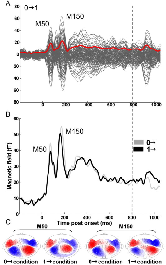
MEG data. A, Example of measured data: grand average (average over all subjects for each of the 160 channels; in gray) of the evoked auditory cortical responses to 0→1 stimuli. The RMS over all channels is plotted in red. B, Group RMS in the right hemisphere for 0→ (gray) and 1→ (black) stimuli (collapsed across the different IAC step sizes). C, Contour maps from the grand-average data at the critical time periods (7.5 fT/isocontour). Source is shown in red; sink is shown in blue. Onset responses to correlated (1→) and uncorrelated (0→) stimuli were comparable. Both are characterized by a two-peaked noise-onset response at ∼70 ms (M50) and 170 ms (M150) after onset, with similar magnetic field distributions. A notable difference is that M50 and M150 peak amplitudes for each subject were significantly stronger for uncorrelated than correlated noise. The difference in the RMS amplitude between A and B is a result of A being computed from the grand-averaged data, whereas B is group RMSs (RMSs of individual subject's RMSs). All statistical analyses were performed on each hemisphere subject-by-subject (based on the 20 channels selected for each). The grand-average plot is shown here for illustration purposes only.

The onset response consisted of two peaks, at ∼70 ms (M50) and ∼170 ms (M150), visible in the grand-averaged data in Figure 4A, both with a spatial distribution characteristic of a standard M50 stimulus-onset response (Woldorff et al., 1993; Yvert et al., 2001; Chait et al., 2004). Interestingly, the M100 peak, with a spatial distribution opposite that of the M50, which is usually seen at ∼100 ms after onset for similar stimuli, is greatly reduced here. There appears to be a small deflection for some subjects, but, in the RMS, it is shadowed by the much stronger M50 and M150 responses. This is in contrast to reports by others that describe noise-onset responses dominated by a M100 peak (Soeta et al., 2004). The lack of an M100 is not the effect of channel selection, because the M100 peak is also absent in the RMS over all channels (Fig. 4A). Rather, it seems to result from the fact that the subjects' task (detection of modulation in the final portion of decoy stimuli) directed their attention away from the onset. This question has been addressed in a previous study (Chait et al., 2004). Overall, results suggest that control of the task, performed by subjects during recording of brain responses, may have a greater importance than is commonly realized.

Onset responses to initial correlated and initial uncorrelated conditions are similar in latency and spatial distribution but with an amplitude stronger for uncorrelated (IAC = 0) than correlated (IAC = 1) noise. Figure 4B shows the group RMS (RMS of individual-subject RMSs) to 1→ and 0→ conditions (collapsed across the different IAC step sizes) in the right hemisphere (RH). Paired sample t tests revealed that M50 and M150 peak amplitudes were significantly stronger for uncorrelated than correlated noise in both hemispheres [df = 17; RH, M50, t = 2.099, p = 0.051; M150, t = 2.704, p = 0.015; left hemisphere (LH), M50, t = 2.298, p = 0.035; M150, t = 3.045, p = 0.007]. This finding is perhaps surprising, given that amplitudes of onset responses are positively related to loudness (Roberts et al., 2000) and that correlated noise evokes a relatively loud compact percept, whereas uncorrelated noise is perceived as less loud and more diffuse (Blauert and Lindemann, 1986). At the same time, it is in agreement with the equalization–cancellation model (Durlach, 1963) that proposes that the inputs to the two ears are subtracted from each other, and the remainder constitutes the representation of binaural information. Another possible interpretation of this finding is that, because the inputs at the two ears do not fuse to a single image, additional neuronal activity is involved in “sorting out” these distributed images. This interpretation is consistent with the shape of EEG binaural interaction components (BICs) of auditory brainstem responses, computed as the difference between the response to binaural stimulation and the sum of the responses to monaural stimulations of the two ears (Polyakov and Pratt, 1998). BICs are usually negative [the binaural response is smaller than the sum of the monaural responses (Krumbholz et al., 2005)] and are of greater amplitude for correlated noise than uncorrelated noise (Polyakov and Pratt, 1998), suggesting that activity evoked by binaurally uncorrelated signals undergoes less mutual suppression than activity evoked by correlated signals.

Soeta et al. (2004) also found that uncorrelated noise onsets evoked a stronger response than correlated noise onsets. However, in their study, stimuli with an IAC of 1 and an IAC of <1 were alternated, which complicates the interpretation of the results: the weaker responses to stimuli with an IAC of 1 may be a result of adaptation, and stronger response for stimuli with a lower IAC may result from the larger interaural correlation difference with the stimulus that preceded them. In an fMRI study using stimuli with fixed IAC values, Budd et al. (2003) identified a distinct subdivision of lateral HG that exhibited a significant positive relationship between blood oxygenation level-dependent (BOLD) activity and IAC. Activation differences were larger for IACs near 1 than those near 0. The trend is opposite of that found in the present study. The apparent discrepancy may result from the current lack of understanding of how hemodynamic BOLD responses are related to the electrical physiological brain responses measured by MEG.

Auditory cortical sensitivity to changes in interaural correlation

The transient response attributable to stimulus onset is followed by a gradual decline to steady-state levels (Fig. 5A). The change in interaural correlation at 800 ms produces a response that rides on this gradual decline, consisting of a prominent peak at ∼950 ms after onset (150 ms after change). To quantify the cortical response to changes in interaural correlation, we subtracted, for each subject and each condition, the time-average amplitude in the 600–800 ms interval from the time-average amplitude in the 850–1050 ms interval (Fig. 5A). For stimuli for which there was an interaural correlation change, we then subtracted from this statistic its value for the corresponding control condition (1→1 or 0→0), for which there was no change in the stimulus. A value significantly different from 0 indicates that auditory cortical activity was affected by the interaural correlation change. Figure 5B shows the computed difference for each of the change conditions in the left and right hemispheres. An ANOVA revealed main effects of reference correlation (F_(1,17) = 10.104; p = 0.005) and size of IAC step (F_{(3.032,51.537)} = 9.829; p < 0.001): differences were larger for larger IAC step sizes and also larger for steps from an initial correlated (IAC = 1) than uncorrelated (IAC = 0) noise. Cortical responses thus parallel ease of detection, as measured behaviorally by both accuracy and reaction times. For 1→ conditions, all differences were significant in both hemispheres (planned comparison, df = 17; LH, 1→0, t = 4.465, p < 0.001; 1→0.2, t = 3.909, p = 0.001; 1→ 0.4, t = 3.237, p = 0.005; 1→0.6, t = 2.229, p = 0.04; 1→0.8, t = 3.205, p = 0.005; RH, 1→0, t = 4.858, p < 0.001; 1→0.2, t = 3.366, p = 0.004; 1→0.4, t = 3.235, p = 0.005; 1→0.6, t = 2.773, p = 0.013; 1→0.8, t = 2.242, p = 0.039). In the case of 0→ conditions, differences were significant for 0→1 and 0→0.8 in the left hemisphere (planned comparison, df = 17; 0→1, t = 4.719, p < 0.001; 0→0.8, t = 2.539, p = 0.021) and for 0→1, 0→0.8, and 0→0.6 in the right hemisphere (df = 17; 0→1, t = 4.281, p < 0.001; 0→0.8, t = 2.296, p = 0.035; 0→0.6, t = 3.102, p = 0.006).

Figure 5.

Auditory cortical sensitivity to changes in interaural correlation. A, Schematic example of the procedure used to quantify sensitivity. The figures present, as an example, the group RMS in the right hemisphere for 0→1 (top panel) and 1→0 (bottom panel) conditions and their controls (0→0 and 1→1, respectively). To quantify the cortical response to changes in interaural correlation, we subtracted, for each subject and each condition, the time-average amplitude in the 600–800 ms interval (PRE) from the time-average amplitude in the 850–1050 ms interval (POST), such that DIFF = POST–PRE. Positive DIFF indicates an increase in activity relative to the activity before the change in IAC. For stimuli for which there was an interaural correlation change, we then subtracted from this statistic its value for the corresponding control condition (1→1 or 0→0) for which there was no change. B, Computed difference for each of the change conditions (0→ conditions in the top panel; 1→ conditions in the bottom panel) in the left (darker shades) and right (lighter shades) hemispheres. Plotted values are the difference between DIFF values in the change conditions versus control conditions. Positive differences indicate that activity after change in IAC was significantly higher than activity after 800 ms in the control condition. Differences that are significantly different from 0 are marked with an asterisk. Error bars represent 1 SE. These physiological responses resemble behavioral responses in that they are larger for correlated than uncorrelated references and for larger changes in correlation.

Figure 6 shows the group RMS of auditory cortical responses to IAC change for 0→1 and 1→0 conditions (other conditions showed a similar response pattern). The change in correlation in the 1→ conditions was characterized by a response with three peaks, ∼70 ms (window 1), ∼130 ms (window 2), and ∼200 ms (window 3) after change. A deflection is considered a “peak” if it is consistent across subjects (see Materials and Methods) and has a salient dipolar distribution that is compatible with activity in auditory cortex. The isocontour magnetic field distribution maps from the grand-average data are also displayed in Figure 6. In contrast, the 0→ condition evoked only one pronounced peak, occurring at a time corresponding to window 2 (Fig. 6B). Thus, window 1 contains the first dipolar response to the 1→ transition, whereas the same window shows no coherent response in the 0→ condition. Window 2 shows a prominent peak for 0→, but, remarkably, the dipolar distribution is of opposite polarity from 1→, indicating that activity cannot possibly be resulting from the same neural substrate. Note also that it is of opposite polarity from that in window 1 for 1→. Thus, the later initial response for 0→ does not merely reflect a delayed activation of the same source. In total, these data suggest that the entire sequence of cortical activation involves distinct neural mechanisms in each case: the mechanism that processes transitions from an IAC of 1 is different from the mechanism that processes transitions from an IAC of 0. These data are consistent with observations reported in an EEG study by Jones et al. (1991), and their different conclusions are attributable to technological limitations at that time.

Figure 6.

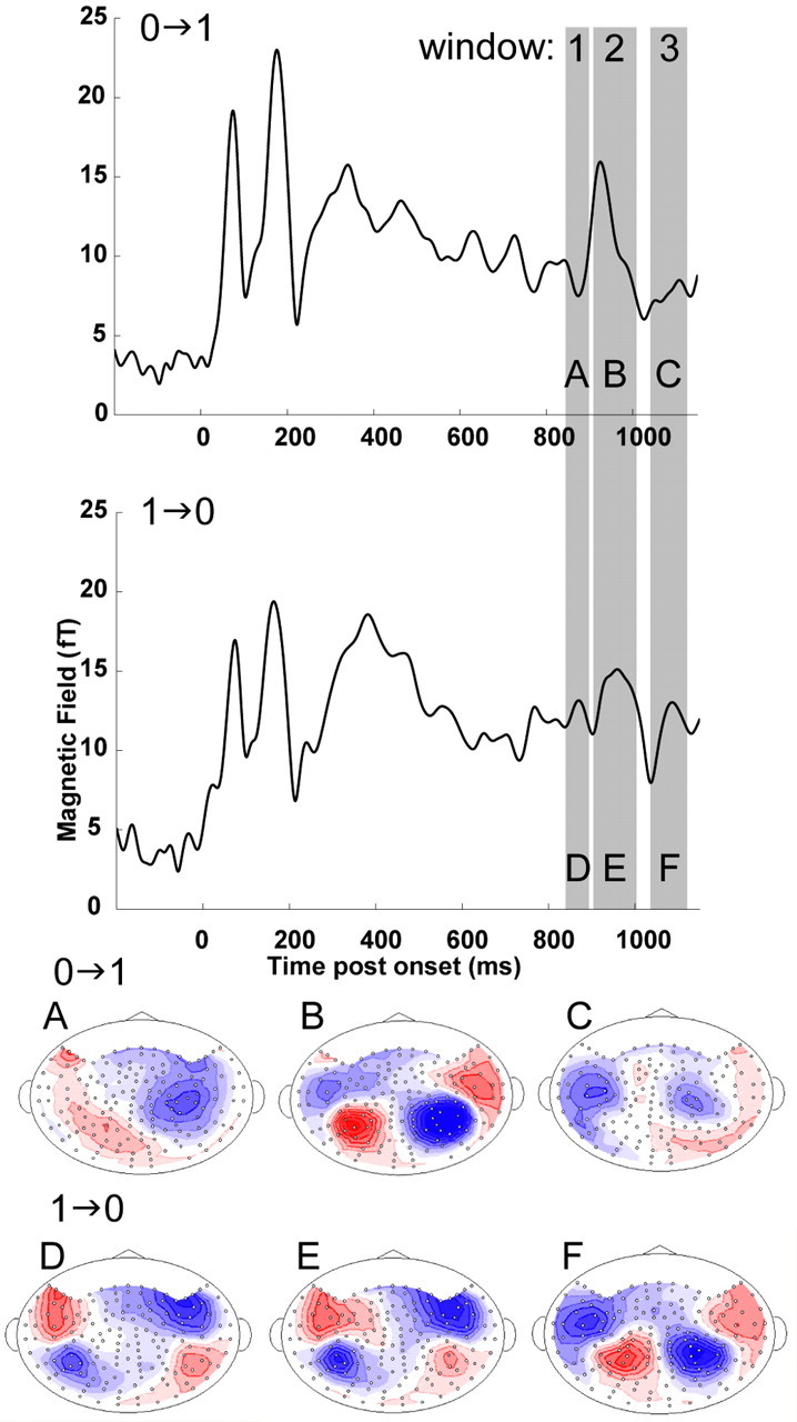
RMS (computed over all channels from the grand-average data) of the auditory cortical responses to 0→1 and 1→0 conditions (other conditions show similar response patterns). The response to the change in correlation was characterized by sequential increases in activity in three temporal windows, ∼70 ms (window 1), ∼130 ms (window 2), and ∼200 ms (window 3) after change in correlation. A–F, The isocontour magnetic field distribution maps from the grand-average data at the critical time periods (7.5 fT/isocontour). Source is shown in red; sink is shown in blue. The responses in the 1→ and 0→ conditions exhibit different magnetic contour map patterns, such that 1→ have pronounced dipolar activity in all three time windows (D–F), but 0→ has a dipolar pattern only in time window 2 (B).

The first observed peak for the 1→ conditions (at ∼850 ms; window 1) occurs ∼80 ms earlier than the first observed peak in the 0→ conditions (at ∼930 ms; window 2). This electrophysiological latency difference may underlie the ∼80 ms response time difference observed in our behavioral data. However, the opposite polarities of these “first responses” are a puzzle. One possibility is that behavior is contingent on the activity within distinct neural substrates reflected in windows 1 (for 1→) and 2 (for 0→). Another possibility is that it is contingent on the same neural substrates, but the activity, visible in window 1 for 1→ conditions, is either weaker in 0→ conditions or delayed and masked by a later activation specific to 0→ conditions (visible in window 2). Because the data for all stimuli were acquired under identical experimental conditions with the same listeners, any difference in the responses implies differences in processing mechanisms. Results are inconsistent with a general processor that would respond to any perceptible change in the steady auditory stimulus conditions [as suggested, for example, by Jones et al. (1991)].

In addition to the existence of a coherent dipolar pattern in window 1, the 1→ conditions always had higher amplitude in that window relative to the corresponding 0→ conditions. This effect is shown in Figure 7 for the conditions for which 0→ activity is significantly different from its control (Fig. 5B) (1→0/0→1, 1→0.2/0→0.8, and 1→0.4/0→0.6). Significance was assessed with the Bootstrap method (500 iterations; balanced) (Efron and Tibshirani, 1993), a computationally intensive resampling method that allows the treatment of situations in which the exact sampling distribution of the statistic of interest is unknown. For each subject, the RMS of the 0→ condition was subtracted from the applicable (same IAC distance) 1→ condition and the difference vectors were bootstrapped. We computed the distribution of bootstrap amplitudes at the peak of the mean difference vector in window 1 for each of the three condition pairs (RH, 871, 891, and 883 ms; LH, 887, 874, and 880 ms) and counted the percent of iterations for which the amplitude difference was less than or equal to zero (perct). A value of perct that is lower than the a priori set 5% level was considered to indicate a significantly higher amplitude in the 1→ conditions relative to the corresponding 0→ conditions (RH, 0→1/1→0, perct = 2.6%; 0→0.8/1→0.2, perct = 4.6%; 0→0.6/1→0.4, perct = 1.4%; LH, 0→1/1→0, perct = 1.2%; 0→0.8/1→0.2, perct = 4.8%; 0→0.6/1→0.4, perct = 2.8%).

Figure 7.

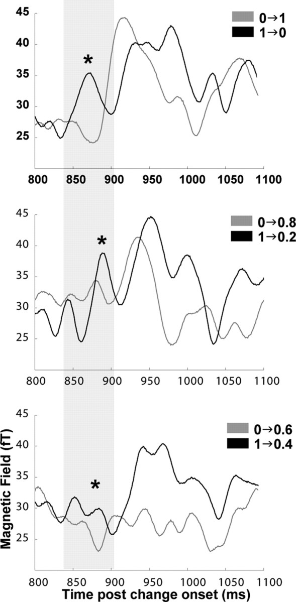
Group RMS in the right hemisphere of the responses to 1→(black) and 0→(gray) conditions with an equal IAC change (plotting only those 0→ conditions for which the response to IAC change is significantly different from the control condition). The first increase in activity is evident in all 1→ conditions at ∼50 ms after a change in correlation. Amplitudes in this time window are significantly stronger for 1→ conditions than for 0→ conditions with a same-sized change in IAC. Asterisks indicate the position of significant differences.

Discussion

We used behavioral methods and whole-head MEG recording to measure responses to the same binaural wideband noise stimuli. For a given step size in interaural correlation, subjects detected transitions from an IAC of 1 more accurately and rapidly than from an IAC of 0. This is consistent with previous studies (Pollack and Trittipoe, 1959a,b; Gabriel and Colburn, 1981; Culling et al., 2001) reporting that equal steps in IAC are not equally salient perceptually in the vicinity of IACs of 0 and 1. However, our results go further by showing an effect of the sign of IAC change, most clearly obvious for the symmetric 1→0 and 0→1 stimuli. This suggests that IAC discriminability might not be adequately described by distance along an internal decision axis because a distance is, by definition, symmetric. A similar asymmetry is prominent in brain responses.

Our behavioral task required subjects to detect a change in interaural correlation, whereas the cortical responses were passive responses to IAC change. Nevertheless, the relationship between the strength of the measured cortical responses to the different conditions (Fig. 5B) paralleled behavioral performance (Fig. 3A): brain responses were more sensitive to transitions from an IAC of 1 (1→ conditions) than to transitions from an IAC of 0 (0→ conditions). Sensitivity in all cases increased with IAC difference. In this respect, our behavioral and brain studies are consistent with each other and with previous literature. In addition, the first salient response to steps from an IAC of 1 occurred earlier than from an IAC of 0, which parallels the latencies measured behaviorally and may conceivably be the neural correlate of the observed behavioral response-time difference. Overall, the earliest observed cortical responses already reflected the asymmetry seen in behavior. What is new is the conclusion, derived from the different polarities of the magnetic field distribution, that 1→ and 0→ transitions evoke activity within different cortical circuits. This result is unexpected, because one would assume all aspects of IAC processing (and changes thereof) to engage common binaural processing mechanisms, and it may shed light on the nature of the computing involved. This finding should be replicable in fMRI (previous studies used fixed IAC values) as well as in physiology.

The 1→ and 0→ conditions differ in both the direction of IAC change (increase or decrease) and in the value of initial correlation (1 or 0). The present study cannot determine whether the observed differential processing is related to the reference correlation or the direction of correlation change. This issue can be resolved in future experiments by studying stimuli with initial correlations different from 0 or 1 (such as 0.5→0 vs 0.5→1 or 0.8→1vs1→0.8).

It is unclear at which level the split into distinct processing streams or the introduction of the 80 ms latency difference between 1→ and 0→ conditions occurs. The MEG responses we record originate from auditory cortex. The computation of interaural correlation is thought to begin at the MSO, where information from the two ears converges on coincidence detectors that perform a form of interaural cross-correlation (Jeffress, 1948; Yin and Chan, 1990; Carr, 1993; Joris et al., 1998). From there, the binaural information pathway projects to the inferior colliculus (IC), medial geniculate body, and cortex. Animal electrophysiological recordings at MSO are rare, but recordings in the IC show correlates of binaural unmasking (Jiang et al., 1997a,b; Palmer et al., 2000) and responses that are influenced by the interaural correlation of stimuli (Palmer et al., 1999). The question arises as to whether sensitivity to binaural coherence is determined by processes at IC (in the same way that basic masking is determined by processes in the auditory nerve), and relayed from there, or if later stages are involved in measuring interaural correlation.

An aspect of interaural correlation processing that has been hypothesized to involve cortical mechanisms and may be related to processes observed here is “binaural sluggishness”: it has been demonstrated that human listeners become less sensitive to time-varying changes in interaural correlation as the change rate is increased (Grantham, 1982). This suggests that listeners compute the effective IAC value over a binaural integration window that, in turn, influences detection in binaural unmasking situations (Grantham and Wightman, 1979; Culling and Summerfield, 1998; Akeroyd and Summerfield, 1999). P. X. Joris, B. van de Sande, A. Recio-Spinoso, and M. van der Heijden (unpublished observations) did not find correlates of sluggishness in IC: single units followed modulations of IAC at rates an order of magnitude higher than the behavioral threshold, suggesting that the site of temporal integration is higher upstream, possibly in cortex.

Binaural sluggishness may be functionally justified by the need to acquire binaural information over a time sufficient to eliminate random fluctuations. These temporal integration mechanisms may underlie the cortical processing speed difference observed here. As discussed above, Joris, van de Sande, Recio-Spinoso, and van der Heijden (unpublished observations) showed that IC neurons react promptly to IAC changes. The longer time it takes cortical mechanisms to respond to one condition versus another can be explained in terms of a central system that integrates the instantaneous information received from IC over time until it has reached a sufficient level of reliability (Shinn-Cunningham and Kawakyu, 2003). The amount of temporal integration may be constant or may vary depending on the stimulus and/or task. For example, supposing that activity over a population of neurons within the MSO is accurately represented by the stimulus cross-correlograms in Figure 1, a mechanism that scans this activity would be able to respond relatively soon after a change from a reference correlation of 1 (Fig. 2A), because such a change “destroys” the orderly arrangement of ridges and valleys that characterizes the response to correlated noise. Conversely, the opposite change (0→1) would take longer to detect because uncorrelated noise is already characterized by random changes in the activation across the neural array; therefore, it would require more time to determine that the sudden order in the stimulus is not merely a random fluctuation. A similar account can also be provided in terms of the equalization–cancellation model (Durlach, 1963): if binaural information is represented as subtraction from the two ears, binaural noise with an IAC of 1 would be represented as an 800-ms-long zero, whereas noise with an IAC of 0 would be represented as an 800-ms-long activation with high variability. For 1→0 stimuli, the change after 800 ms would be evident as a sudden change from 0 to a positive number. For 0→1, the change at 800 ms is preceded by random fluctuations, and the system would need to wait longer to detect it.

Response latencies measured in auditory cortex provide an upper limit for the size of the binaural integration window: ∼50 ms for transitions from correlated noise and ∼130 ms for transitions from uncorrelated noise. These estimates are similar to those derived from behavioral measurements (Culling and Summerfield, 1998; Akeroyd and Summerfield, 1999; Boehnke et al., 2002). The different integration times required for 1→ and 0→ transitions might conceivably be implemented by a single mechanism with a variable integration time. Another possibility is that the process passes via two successive integration mechanisms: an initial obligatory integration window and a subsequent integration window, provided by a separate neural substrate, that is only required in the 0→ condition to reach a sufficient level of certainty that there has been a change. Such a model would explain the activation of distinct neural populations for the two kinds of transitions.

That it takes longer to react to changes from a disordered state to an ordered state than vice versa may be a general attribute of perceptual phenomena. For example, data on the perception of dynamic random-dot stereograms (Julesz and Tyler, 1976) are very similar to those obtained in the auditory domain with noise signals. The visual stimuli strongly parallel ours, consisting of frame sequences in which the left and right frames are either identical [interoccular correlation (IOC) = 1] or uncorrelated (IOC = 0). Subjects' ability to detect changes in IOC from 0 to 1 and vice versa reveal an asymmetry, similar to the results presented here. Julesz and Tyler (1976) liken this effect to the physical concept of entropy: perceptual phenomena require more effort/time to build up representations (go to an orderly state) than to destroy them (go to a less ordered state). This account also offers an additional interpretation to the observed three-staged processing of changes in interaural correlation. The first peak (window 1), only visible in the 1→ conditions, may reflect the destruction of the representation of the correlated noise, whereas the second peak (window 2), visible in both conditions but having different source properties, may underlie the construction (or attempts at the construction) of a new perceptual order.

The strong similarities in detecting changes in correlation between vision and audition may indicate that the statistical rules that determine the size of the integration windows are modality independent and are not special to a particular neural substrate. This observation, together with the findings reported here, may provide a basis for additional examinations of how the CNS computes and represents changes in the environment.

References

- Adachi Y, Shimogawara M, Higuchi M, Haruta Y, Ochiai M (2001) Reduction of non-periodic environmental magnetic noise in MEG measurement by continuously adjusted least squares method. IEEE Trans Appl Superconduct 11: 669–672. [Google Scholar]
- Akeroyd MA (2001) Binaural-modeling software for MATLAB/Windows; http://www.ihr.gla.ac.uk/products/matlab.php.
- Akeroyd MA, Summerfield Q (1999) A binaural analog of gap detection. J Acoust Soc Am 105: 2087–2820. [DOI] [PubMed] [Google Scholar]
- Blauert J, Lindemann W (1986) Auditory spaciousness: some further psychoacoustic analyses. J Acoust Soc Am 80: 533–541. [DOI] [PubMed] [Google Scholar]
- Boehnke SE, Hall SE, Marquardt T (2002) Detection of static and dynamic changes in interaural correlation. J Acoust Soc Am 110: 1617–1626. [DOI] [PubMed] [Google Scholar]
- Budd TW, Hall DA, Goncalves MS, Akeroyd MA, Foster JR, Palmer AR, Head K, Summerfield AQ (2003) Binaural specialisation in human auditory cortex: an fMRI investigation of interaural correlation sensitivity. NeuroImage 20: 1783–1794. [DOI] [PubMed] [Google Scholar]
- Carr CE (1993) Processing of temporal information in the brain. Annu Rev Neurosci 16: 223–243. [DOI] [PubMed] [Google Scholar]
- Chait M, Simon JZ, Poeppel D (2004) Auditory M50 and M100 responses to broadband noise: functional implications. NeuroReport 15: 2455–2458. [DOI] [PubMed] [Google Scholar]
- Colburn HS (1995) Computational models of binaural processing. In: Springer handbook of auditory research, Vol 6, Auditory computation (Hawkins HL, McMullen TA, Popper AN, Fay RR, eds), pp 332–400. New York: Springer.
- Culling JF, Summerfield Q (1998) Measurements of the binaural temporal window using a detection task. J Acoust Soc Am 103: 3540–3553. [Google Scholar]
- Culling JF, Colburn HS, Spurchise M (2001) Interaural correlation sensitivity. J Acoust Soc Am 110: 1020–1029. [DOI] [PubMed] [Google Scholar]
- Durlach NI (1963) Equalization and cancellation theory of binaural masking-level differences. J Acoust Soc Am 35: 1206–1218. [Google Scholar]
- Durlach NI, Gabriel KJ, Colburn HS, Trahiotis C (1986) Interaural correlation discrimination. II. Relation to binaural unmasking. J Acoust Soc Am 79: 1548–1557. [DOI] [PubMed] [Google Scholar]
- Efron B, Tibshirani RJ (1993) An introduction to the Bootstrap. New York: Chapman and Hall.
- Gabriel KJ, Colburn HS (1981) Interaural correlation discrimination. I. Bandwidth and level dependence. J Acoust Soc Am 69: 1394–1401. [DOI] [PubMed] [Google Scholar]
- Grantham DW (1982) Detectability of time-varying interaural correlation in narrow-band noise stimuli. J Acoust Soc Am 72: 1178–1184. [DOI] [PubMed] [Google Scholar]
- Grantham DW, Wightman FL (1979) Detectability of a pulsed tone in the presence of amasker with time-varying interaural correlation. J Acoust Soc Am 65: 1509–1517. [DOI] [PubMed] [Google Scholar]
- Greenhouse SW, Geisser S (1959) On methods in the analysis of profile data. Psychometrika 24: 95–112. [Google Scholar]
- Hämäläinen M, Hari R, Ilmoniemi RJ, Knuutila J, Lounasmaa OV (1993) Magnetoencephalography—theory, instrumentation, and applications to noninvasive studies of the working human brain. Rev Mod Phys 65: 413–497. [Google Scholar]
- Hari R (1990) The neuromagnetic method in the study of the human auditory cortex. In: Auditory evoked magnetic fields and the electric potentials. Advances in audiology, Vol 6 (Grandori F, Hoke M, Romani GL, eds), pp 222–282. Basel: Karger. [Google Scholar]
- Hirsh IJ (1948) The influence of interaural phase on interaural summation and inhibition. J Acoust Soc Am 20: 536–544. [Google Scholar]
- Jeffress LA (1948) A place theory of sound localization. J Comp Physiol Psychol 41: 35–39. [DOI] [PubMed] [Google Scholar]
- Jiang D, McAlpine D, Palmer AR (1997a) Responses of neurons in the inferior colliculus to binaural masking level difference stimuli measured by rate-versus-level functions. J Neurophysiol 77: 3085–3106. [DOI] [PubMed] [Google Scholar]
- Jiang D, McAlpine D, Palmer AR (1997b) Detectability index measures of binaural masking level difference across populations of inferior colliculus neurons. J Neurosci 17: 9331–9339. [DOI] [PMC free article] [PubMed] [Google Scholar]
- Jones SJ, Pitman JR, Halliday AM (1991) Scalp potentials following sudden coherence and discoherence of binaural noise and change in the interaural time difference: a specific binaural evoked potential or a “mismatch” response? Electroencephalogr Clin Neurophysiol 80: 146–154. [DOI] [PubMed] [Google Scholar]
- Joris PX, Smith PH, Yin TC (1998) Coincidence detection in the auditory system: 50 years after Jeffress. Neuron 21: 1235–1238. [DOI] [PubMed] [Google Scholar]
- Julesz B, Tyler CW (1976) Neurontropy, an entropy-like measure of neural correlation, in binocular fusion and rivalry. Biol Cybern 23: 25–32. [DOI] [PubMed] [Google Scholar]
- Krumbholz K, Schonwiesner M, Rubsamen R, Zilles K, Fink GR, von Cramon DY (2005) Hierarchical processing of sound location and motion in the human brainstem and planum temporale. Eur J Neurosci 21: 230–238. [DOI] [PubMed] [Google Scholar]
- Licklider JCR (1948) The influence of interaural phase relations upon the masking of speech by white noise. J Acoust Soc Am 20: 150–159. [Google Scholar]
- Lütkenhöner B, Steinsträter O (1998) High-precision neuromagnetic study of the functional organization of the human auditory cortex. Audiol Neurootol 3: 191–213. [DOI] [PubMed] [Google Scholar]
- McAlpine D, Grothe B (2003) Sound localization and delay lines— do mammals fit the model? Trends Neurosci 26: 347–350. [DOI] [PubMed] [Google Scholar]
- Moore BC, Glasberg BR (1983) Suggested formulae for calculating auditory-filter bandwidths and excitation patterns. J Acoust Soc Am 74: 750–753. [DOI] [PubMed] [Google Scholar]
- Oldfield RC (1971) The assessment and analysis of handedness: the Edinburgh inventory. Neuropsychologia 9: 97–113. [DOI] [PubMed] [Google Scholar]
- Palmer AR, Jiang D, McAlpine D (1999) Desynchronizing responses to correlated noise: a mechanism for binaural masking level differences at the inferior colliculus. J Neurophysiol 81: 722–734. [DOI] [PubMed] [Google Scholar]
- Palmer AR, Jiang D, McAlpine D (2000) Neural responses in the inferior colliculus to binaural masking level differences created by inverting the noise in one ear. J Neurophysiol 84: 844–852. [DOI] [PubMed] [Google Scholar]
- Pantev C, Bertrand O, Eulitz C, Verkindt C, Hampson S, Schuierer G, Elbert T (1995) Specific tonotopic organizations of different areas of the human auditory cortex revealed by simultaneous magnetic and electric recordings. Electroencephalogr Clin Neurophysiol 94: 26–40. [DOI] [PubMed] [Google Scholar]
- Pollack I, Trittipoe WJ (1959a) Binaural listening and interaural noise cross correlation. J Acoust Soc Am 31: 1250–1252. [Google Scholar]
- Pollack I, Trittipoe WJ (1959b) Interaural noise correlations: Examination of variables. J Acoust Soc Am 31: 1616–1618. [Google Scholar]
- Polyakov A, Pratt H (1998) The effect of binaural masking noise disparity on human auditory brainstem binaural interaction components. Audiology 37: 17–26. [DOI] [PubMed] [Google Scholar]
- Roberts TP, Ferrari P, Stufflebeam SM, Poeppel D (2000) Latency of the auditory evoked neuromagnetic field components: stimulus dependence and insights toward perception. J Clin Neurophysiol 17: 114–129. [DOI] [PubMed] [Google Scholar]
- Shinn-Cunningham B, Kawakyu K (2003) Neural representation of cource direction inreverberant space. Paper presented at IEEE Workshop on Applications of Signal Processing to Audio and Acoustics, New Paltz, NY, October.
- Soeta Y, Hotehama T, Nakagawa S, Tonoike M, Ando Y (2004) Auditory evoked magnetic fields in relation to interaural cross-correlation of bandpass noise. Hear Res 196: 109–114. [DOI] [PubMed] [Google Scholar]
- Stern RM, Trahiotis C (1995) Models of binaural interaction. In: Handbook of perception and cognition, Ed 2, Hearing (Moore BCJ, ed), pp 347–386. San Diego: Academic.
- Woldorff MG, Gallen CC, Hampson SA, Hillyard SA, Pantev C, Sobel D, Bloom FE (1993) Modulation of early sensory processing in human auditory cortex during auditory selective attention. Proc Natl Acad Sci USA 90: 8722–8726. [DOI] [PMC free article] [PubMed] [Google Scholar]
- Yin TC, Chan JC (1990) Interaural time sensitivity in medial superior olive of cat. J Neurophysiol 64: 465–488. [DOI] [PubMed] [Google Scholar]
- Yvert B, Crouzeix A, Bertrand O, Seither-Preisler A, Pantev C (2001) Multiple supratemporal sources of magnetic and electric auditory evoked middle latency components in humans. Cereb Cortex 11: 411–423. [DOI] [PubMed] [Google Scholar]