Neuronal dynamics regulating brain and behavioral state transitions

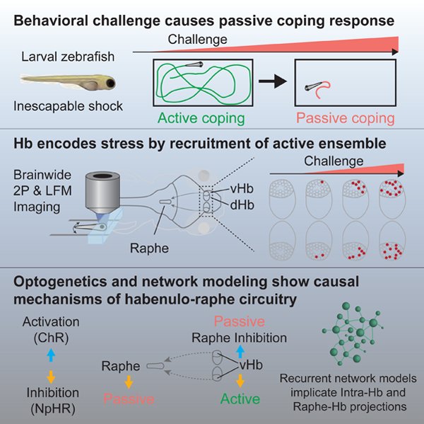
Abstract

Prolonged behavioral challenges can cause animals to switch from active to passive coping strategies, to manage effort-expenditure during stress; such normally-adaptive behavioral state transitions can become maladaptive in psychiatric disorders such as depression. The underlying neuronal dynamics and brainwide interactions important for passive coping have remained unclear. Here, we develop a paradigm to study these behavioral state transitions at cellular-resolution across the entire vertebrate brain. Using brainwide imaging in zebrafish, we observed that the transition to passive coping is manifested by progressive activation of neurons in the ventral (lateral) habenula. Activation of these ventral-habenula neurons suppressed downstream neurons in the serotonergic raphe nucleus and caused behavioral passivity, whereas inhibition of these neurons prevented passivity. Data-driven recurrent neural network modeling pointed to altered intra-habenula interactions as a contributory mechanism. These results demonstrate ongoing encoding of experience features in habenula, which guides recruitment of downstream networks and imposes a passive coping behavioral strategy.

Graphical Abstract

eTOC

Brainwide imaging in zebrafish and network modeling reveal that switching from active to passive coping state arises from progressive activation of habenular neurons in response to behavioral challenge.

Introduction

Prior experience affects how future actions are evaluated and selected; this feedback is essential to reinforcement learning algorithms and is critical for generating adaptive behaviors (Sutton and Barto, 1998). Aversive or stressful experiences can be particularly important in shaping future decisions, and individuals will reliably select actions intended to counteract an aversive stimulus. However, when such actions fail to counteract the stimulus, individuals may choose to adaptively suppress the actions. Repeated failure of actions to produce value can result in a deep discounting of the value of effort in the present; in human beings, this discounting is maladaptive when manifesting as hopelessness, one of the core clinical criteria of major depressive disorder (American Psychiatric Association, 2000; Beck et al., 1985).

The mechanisms governing action selection in the face of stressors can be studied with behavioral challenge (BC) assays; animals exposed to inescapable aversive environments initially attempt vigorous escape actions, but eventually transition to a passive coping (PC) state (Koolhaas et al., 1999) characterized by reduced mobility (Porsolt et al., 1978; Steru et al., 1985). A behavioral transition to PC is consistent with the discounting of the value of effort (Nestler and Hyman, 2010; Warden et al., 2012), and is modulated by genetic, behavioral, and pharmacological interventions related to depression (Cryan et al., 2005; Willner, 2005).

Several brain regions have been proposed to play a role in governing the PC response (Shumake and Gonzalez-Lima, 2003), including the prefrontal cortex (Maier and Watkins, 2010; Warden et al., 2012), lateral septum (Anthony et al., 2014), basal ganglia (Shabel et al., 2012; Stephenson-Jones et al., 2016), periaqueductal gray (Bandler et al., 2000), hypothalamus (Wang et al., 2015), raphe nuclei (Roche et al., 2003; Yang et al., 2008), ventral tegmental area (Stamatakis and Stuber, 2012; Tye et al., 2013) and habenula (Cui et al., 2018; Lee et al., 2010; Li et al., 2011; Okamoto et al., 2012; Proulx et al., 2014; Shumake et al., 2004; Yang et al., 2008, 2018). However, it remains unclear where and how relevant evidence regarding the ongoing behavioral experience is encoded across the brain during BC, and how the resulting transition from active coping (AC) to PC is causally manifested from this evidence. These questions are challenging to address, owing to the distributed spatial arrangement of the relevant regions across the brain, and the inability to perform brainwide cellular-resolution neuronal activity imaging in mammals.

We therefore established a novel BC protocol for larval zebrafish, with small size and near-transparency permitting brainwide cellular-resolution neural activity imaging (Ahrens et al., 2012; Vladimirov et al., 2014) and facilitating data-driven circuit models (Naumann et al., 2016). Zebrafish brains contain key regions associated with PC in rodents, including the conserved habenulo-raphe pathway (Amo et al., 2010; Hikosaka, 2010; Namboodiri et al., 2016). Like the mammalian habenula (Hb), the zebrafish Hb is subdivided into two parts, the dorsal (dHb) and ventral (vHb) portions, which are homologous to the mammalian medial (MHb) and lateral (LHb) portions, respectively (Agetsuma et al., 2010; Amo et al., 2010; Lee et al., 2010).

We find in larval zebrafish a PC response characterized by immobility that is modulated by anti-depressant treatment and prior experience. We use the discovery of this conserved process to collect brainwide cellular-resolution recordings of neural activity during BC and probe the causal effects of the observed activity through optogenetics and computational modeling, revealing neuronal dynamics across a network of brain regions that encodes the ongoing negative experience of BC and transitions the animal to a PC behavioral state.

Results

Behavioral challenge induces passive coping in zebrafish

We developed a BC protocol that, similar to related rodent protocols, relied on exposing animals to an inescapable adverse environment. Fish 10–15 days post fertilization (dpf) were placed in a small plastic tank and tracked while being exposed to repeated mild shocks (1Hz for 30 minutes) (Figure 1A). We observed that fish initially displayed a significant increase in movement following the onset of shock, but, over time, entered a state in which they moved significantly less than fish that were not shocked (Figure 1B–1D; Movie S1). This transition from increased to decreased movement parallels the transition from AC to PC observed in challenged rodents (Warden et al., 2012).

Figure 1: Active-to-passive coping behavioral state transition in larval zebrafish.

(A) BC rig tracks fish position and delivers electric shocks (B and C) The behavioral response of two fish: 0V control fish (B) and 5V shocked fish (C). The path during the pre-shock period (purple) and the post-shock period (orange) (upper left, scale bar = 10 mm). The position along the short (upper right) and long (lower left) sides of tank over the entire protocol (pink shading indicates shock period). Speed of fish in 60 s windows (lower right) shows that BC results in reduced movement. (D) Shocked fish (blue, n=33) increased their speed (AC) in response to the first five minutes of BC (p=5.15 × 10⁻⁶) then transitioned to a reduced mobility state (PC) compared to controls (black, n=14; p=7.03 × 10⁻⁸ at final time point). See also Figure S1A. (E) Fish context was changed post-BC to assess recovery rate (transition indicated with dashed lines). Fish moved to the neutral context (blue) recovered to the level of control fish kept in the same tank (black; p=0.11, n.s.; One-way ANOVA with Holm-Sidak post-hoc comparison; data also in panel D), while fish returned to the aversive context (green, n=40) or the partially-neutral context (yellow, n=29) did not recover compared to shocked fish in the neutral environment (p=2.12 × 10⁻⁸ and p=.003, respectively). (F) Exposure to ketamine one hour before BC (n=16) reduced and delayed the onset of PC compared to controls (n=8, p<0.05 between 7 and 17 minutes post shock), but did not fully prevent the transition when fish were exposed to a longer BC protocol. See also Figure S1B and S1C. In all figures, shaded area and error bars indicate standard error of the mean (s.e.m.) and all statistical tests are Student’s t-tests, unless otherwise indicated (*P<.05; **P<.01; ***P<.001).

To assess whether reduced movement reflected a change in coping strategy rather than a fear-related freezing behavior or a non-specific effect of shock on physical health, we examined if and how fish regained normal movement levels. Following exposure to the BC protocol, fish were placed in one of three different environments: neutral (a tank of a different color with fresh system water), partially-neutral (the same tank in which they were shocked with fresh system water), and aversive (the same tank and water). We found that in the first 5 minutes after being moved to a neutral context fish showed no significant recovery of swimming speed (Figure 1E and S1A). This result comports with the trans-situationality of PC responses (Porsolt et al., 1978), but is distinct from the immediate recovery from freezing behavior observed in contextual fear assays (Fanselow, 1980). Moreover, over the course of 30 minutes, fish placed in the neutral environment recovered more than fish in both the partially-neutral and aversive environments and eventually moved at a similar rate to control fish. Thus, visual aspects of the environment alone modulated the return to control-level behavior, suggesting that the reduced speed resulting from BC was manifesting a behavioral state akin to PC and not a non-specific effect on health.

In rodents, the transition from AC to PC in response to BC can be delayed by treatment with the acute anti-depressant ketamine (Yilmaz et al., 2002). We therefore examined if this response would be conserved in fish. Fish were exposed to a single dose of ketamine and allowed to recover from the acute effect of the drug for one hour before undergoing BC (Figure S1B). We found that this exposure delayed the reduction in speed compared to non-treated fish, only exhibiting passive behavior in an extended version of the BC protocol (Figure 1F). We found this effect was dose dependent, persisted for at least 4 hr after ketamine treatment, and subsided by 24 hr (Figure S1C). The SSRI fluoxetine also modulated the transition to PC but exhibited an additional effect on baseline spontaneous movement (Figure S1D).

To establish that the reduced speed we observed represented a PC response to inescapable BC, and not a form of habituation to shock, we conducted a closed-loop yoked-control experiment. One cohort of fish could prevent or reduce shocks by performing actions in response to visual cues (Figure S1E), while a second paired cohort experienced an identical pattern of shocks and cues but without any control over shock statistics. We conducted this experiment on fish in two age ranges (10–15 dpf and 21–28 dpf), because the ability to associate a cue or action with an outcome develops at 3 weeks of age in zebrafish (Valente et al., 2012). In the older fish, we found that the inescapable shock cohort stopped responding at trial onset, while the escapable shock cohort showed no such reduction in response (Figure S1F–I). This result was inconsistent with an interpretation of the reduced-movement response to inescapable shock as a form of habituation. In the younger fish, we did not observe this difference as expected given the inability of fish this age to learn simple associations (Valente et al., 2012). Taken together, our behavioral experiments support the view that larval zebrafish can undergo a behavioral state change akin to the PC response characterized in other vertebrate systems.

Whole-brain imaging following behavioral challenge: increased activity in vHb

To begin to map patterns of neural activity associated with the PC response, we used light field microscopy (LFM), a high-speed volumetric imaging technique, to record synchronous whole-brain neural activity following BC (Figure 2A) (Broxton et al., 2013; Levoy et al., 2006; Prevedel et al., 2014). This enabled an unbiased assessment of the resulting neural state. Light fields were collected at 5Hz, reconstructed as 691 × 800 × 500 µm volumes with a voxel size of 3.6 × 3.6 × 5.0 µm, and then motion corrected and aligned to a reference atlas (Figure 2B, S2A and S2B). We imaged transgenic fish expressing the genetically-encoded Ca²⁺ indicator GCaMP6s under the pan-neuronal promoter elavl3 localized to the nucleus, Tg(elavl3:H2B-GCaMP6s) (Vladimirov et al., 2014). Localization of the Ca²⁺ indicator to the nucleus ensured that signals within voxels reflected changes in the activity of co-localized somata, and not activity in neuropil – an important consideration given the spatial resolution of the LFM volumes (Figure S2C–S2E).

Figure 2: Whole-brain Ca²⁺ imaging using LFM: unique vHb hyperactivity following BC.

(A) LFM was used to measure GCaMP6s Ca²⁺ signals during a 45-minute post-BC period. (B) Orthogonal maximum intensity projections of a LFM volume (scale bar = 50µm). Hb: habenula; OT: optic tectum; Fore: forebrain; Oe: olfactory epithelium; Ce: cerebellum; Hind: hindbrain. See also Figure S2. (C) Orthogonal min-max projections of volumes showing the change in fluorescence over the post-BC period in a representative fish from the control group (top), shocked group (middle); and ketamine group (bottom). Red and blue indicate an increase and decrease in fluorescence, respectively (arbitrary units; black arrows show the location of the vHb; scale bar = 50µm). (D) Change in average fluorescence over the post-BC period. Shocked fish showed an increase in vHb activity (blue, n=6) compared to control fish (black, n=4; p=0.0002, two-way repeated-measures ANOVA with Tukey HSD post-hoc comparison). This effect was reduced in shocked fish that were previously treated with ketamine (pink, n=8; p=0.0014).

These recordings revealed that activity in the vHb, alone across the entire brain, exhibited elevation in fish exposed to BC. We examined the fluorescence in several anatomically defined regions (Figure S2F) over 45 minutes following the end of the protocol. Over this period, we observed significantly increased fluorescence in the vHb of shocked fish compared to controls (Figure 2C and 2D). This increasing activity was confined to the vHb and was prevented by treatment with ketamine one hour prior to imaging. To confirm that this finding was not dependent on immobilization of the fish for imaging, we performed in situ hybridization for the immediate early gene c-fos following free-swimming BC and observed a marked increase in c-fos expression within the vHb (Figure S2G and S2H). Our identification of increased activity in the vHb using an unbiased screen of neural activity supports the idea that hyperactivity in the vHb is an important neural correlate of PC behavior (Caldecott-Hazard et al., 1988; Dolzani et al., 2016), and suggests that the neural underpinnings of this behavior are conserved between zebrafish and mammals.

vHb activity is correlated with the extent of behavioral challenge

We next sought to determine how the nature of ongoing negative experience could be encoded by the brain during BC. To ensure that single-cell spatial resolution could be maintained even within dense clusters of neurons, we transitioned to imaging with a resonance-scanning piezo-focus two-photon (2P) microscope. Larval fish were positioned under the microscope objective by head-embedding in agarose and tail-movements were monitored (Figure 3A and 3B). Shocks were delivered via conductive pads on either side of the fish, with their frequency reduced for compatibility with the lower temporal resolution (1–1.2 Hz) of the 2P microscope (inter-shock interval 15 to 25 s). This shock protocol caused a reduction in the frequency of tail movements over the course of the behavioral session that was rescued by prior exposure to ketamine (Figure 3C), and also sufficed to cause free-swimming fish to enter a PC state (Figure S3A). An analysis of shock-triggered neural responses revealed shock-responsive cells in many regions throughout the brain (Figure S3B and S3C).

Figure 3: 2P imaging of cellular-resolution brainwide responses during BC reveal the dynamics of experience-encoding activity in the vHb.

(A) Head-fixed volumetric 2P calcium imaging during BC while monitoring tail movement. (B) Diagram of imaged brain area (yellow rectangle). (C) Head-fixed fish exhibit a reduction in tail movement rate as a result of BC (black: control, n=6; blue: shocked, n=8; p=0.030, one-sided Student’s t-test). Prior exposure to acute ketamine eliminates this response (pink, n=4, p=0.283, n.s.). (D) Regressor consisting of linearly rising activity following the onset of shocks was used to search for cells with activity correlated to the extent of BC. (E) Example of the fit between the regressor and the ∆f/f Ca²⁺ trace for four neurons (bottom; locations at top; black dashed line indicates start of shocks). (F) ROI of each neuron colored by the correlation (r) between its ∆f/f Ca²⁺ trace and the regressor (scale bar = 25 µm). See also Figure S3. (G) Average baseline-subtracted ∆f/f response for all neurons in each of several brain regions (see also Figure S4). In the vHb, the average activity over the final two minutes was increased in shocked fish (n=8) compared to control (n=6) and ketamine-treated (n=4) fish (p=0.0189 and p=0.0432, respectively; two-way repeated-measures ANOVA with Tukey HSD post-hoc comparison). Shocked fish also showed a decrease in raphe activity (p=0.012 and p=0.007) and dorsal thalamus activity (p=0.007 and p=0.006) compared to controls and ketamine-treated fish. (H) Example of MultiMAP registration to identify serotonergic neurons in the superior raphe (see methods). (I and J) Raster plot of baseline-subtracted ∆f/f activity of all 5-HT+ neurons (I; n = 158 neurons from 3 fish) and 5-HT– neurons (J; n = 332 neurons) sorted based on hierarchical clustering with top 8 flat clusters demarcated by coloring scheme of left. 5-HT+ neurons, on average, exhibited a significantly larger response to BC onset compared to 5-HT– neurons (60 second window following onset; p = 0.026, paired Student’s t-test) and compared to 5-HT+ neurons in non-shocked controls (n=4 non-shocked control fish; p = 0.027, Student’s t-test). 5-HT– neurons did not have a significant response to BC onset (p = 0.37, Student’s t-test).

To explore how the BC experience might be represented in brainwide neural activity patterns, we performed a search for cells with activity correlated to the persistence of the challenge. The activity of each cell was fit to a regressor that was flat during the pre-challenge period but rose linearly during challenge (Figure 3D and 3E). This analysis revealed a prominent cluster of positively correlated cells in the vHb of shocked fish (Figure 3F and S3D; Movie S2 and S3). Computing the time-course of average activity across all vHb neurons revealed that activity in the vHb steadily rose over the course of the protocol (Figure 3G, upper left). This increase was not observed in fish previously treated with ketamine despite the fact that the treatment did not alter the percentage of vHb cells that acutely responded to shock (Figure S3E and S3F) (Matsumoto and Hikosaka, 2007). Though certain characteristics of the zebrafish Hb are known to be bilaterally asymmetric (Bianco and Wilson, 2009), the elevation in vHb activity was not significantly different between the two hemispheres (Figure S3G). Our observation of rising vHb activity in response to BC links research suggesting that the Hb encodes aversive expectation value (Amo et al., 2014; Lee et al., 2010) to findings associating vHb hyperactivation with the etiology of depression (Cui et al., 2018; Hu et al., 2013; Li et al., 2011; Yang et al., 2018). The emergence of this observation from unbiased analysis supports its interpretation as an important component of the biological response to BC.

Behavioral challenge causes net inhibition of identified serotonergic raphe neurons

Outside the vHb, we examined neural activity in anatomical regions associated with passivity in other species, in known afferent and efferent targets of the vHb, and in areas where responses to BC were clustered in our regressor analysis (Figure S4). We defined these regions manually in all fish using anatomical landmarks. The region lateral of rhombencephalic neuropil region 6 (Z-Brain Atlas; Randlett et al., 2015) contains the griseum centrale, an area homologous to the mammalian periaqueductal gray, which has been associated with immobility (Bandler et al., 2000; Okamoto et al., 2012). This region showed a significant response at the onset of BC (Figure S5B) but did not show the progressive activation observed in the Hb. The ventral entopeduncular nucleus (vEP, homologous to the globus pallidus in mammals) is a known source of afferents to the vHb (Amo et al., 2014; Shabel et al., 2012; Turner et al., 2016). The region of the telencephalon containing vEP did not show a significant change in overall average activity – though some individual cells did (Figure S3D).

The superior raphe nucleus (combined dorsal and median subdivisions) and dorsal thalamus both showed significant changes in activity in response to BC (Figure 3G). In contrast to the response in the vHb, these responses were inhibitory and exhibited plateau responses. The raphe is the primary downstream target of the vHb in zebrafish (Amo et al., 2010, 2014) and has been implicated in PC responses in other systems (Maier and Seligman, 2016). Thus a change in raphe activity was not surprising, but the direction was not predictable. Slice physiology has shown that optogenetic activation of the vHb causes excitatory responses in serotonergic neurons (Amo et al., 2014), but other work suggests raphe dynamics in response to PC may be more complex due to the diversity of cell types and projections (Amat et al., 2010; Grahn et al., 1999; Lillesaar, 2011; Nathan et al., 2015; Ren et al., 2018; Stern et al., 1979; Teissier et al., 2015).

To further demonstrate the observed inhibitory mechanism, we employed MultiMAP (Lovett-Barron et al., 2017) to specifically identify serotonergic neuron activity within the raphe (Figure 3H). Hierarchical cluster analysis revealed that both the serotonergic and non-serotonergic populations contained a large cluster of neurons that displayed decreased activity similar to the overall raphe population average (Figure 3I and 3J; blue clusters), but the serotonergic population showed a more robust and significant response at the onset of BC as a result of a large set of onset-responding neurons (Figure 3I; blue and yellow clusters). This pattern may bear relevance to clinical distinctions between acute and delayed responses to serotonergic drugs, and may also relate to studies of rodent PC behavior showing that the mPFC-to-LHb and mPFC-to-raphe projection exert opposing effects on BC-elicited passivity (Roche et al., 2003; Warden et al., 2012).

Hb cells are continuously recruited during behavioral challenge

The unique and localized accumulator-like pattern of activity in the vHb suggested a specialized central role in encoding the nature of ongoing adverse experience. To better characterize these Hb dynamics, we investigated if this pattern would be manifested within individual cells or instead represent a composite of diverse cellular responses with distinct dynamics. We examined the activity of those neurons that showed significant activation as a result of BC (Figure 4A) and observed a diversity of activation latencies and durations (Figure 4B). This analysis revealed a striking pattern of staggered recruitment of individual cells, with response latencies tiling the duration of the protocol (Figure 4D; differing from a homogeneous Poisson point process, see Methods), and with many neurons becoming fully activated quickly compared to the duration of the protocol (Figure 4C).

Figure 4: Staggered recruitment of individual vHb neurons temporally tiles BC epoch.

(A) Percentage of neurons that showed a significant increase in activity (top) or decrease in activity (bottom) as a result of BC (black: control, n=6; blue: shocked, n=8; pink: ketamine, n=4; data from these fish also presented in Figure 3). A higher percentage of vHb neurons were excited in shocked fish (p=0.037), while more raphe neurons were inhibited (p=0.048), compared to controls. (B) ∆f/f Ca²⁺ traces (purple) for all vHb neurons that showed a significant increase in activity were smoothed (dark purple) and then fit to a sigmoid (black). 4 example neurons with varying response durations (time between 10^th and 90^th percentile of the sigmoid) and latencies (time to the 50^th percentile) are shown (dashed line is onset of shocks). (C) Histogram of response durations. (D) Histogram of response latencies (excluding neurons with response durations longer than 30 minutes). (E) Raster plot of ∆f/f traces for neurons in panel D from a representative fish sorted by response latency. (F) ROIs of neurons in panel E colored according to their response latency (6µm between sections; scale bar = 25 µm). (J) Histogram of difference in response latency between neighboring neurons and neurons with random spatial locations. The latency difference between neighbors is smaller than expected by chance (n=979 neurons from 8 fish; p=.0005, nonparametric bootstrap, see Methods). (H, I) Analogous to panels C and D for cells showing significantly decreased activity in the raphe. (J) Analogous to panel E for raphe neurons.

These distributions indicated that the rising average activity in the vHb was not the result of a similar slow ramping across all neurons, but rather reflected diverse dynamics in which neurons were recruited with staggered latencies into the activated ensemble (Figure 4E). Interestingly, the time at which an individual neuron was recruited into this ensemble was not independent of its spatial location (Figure 4F); nearby neurons exhibited response times that were significantly more similar than expected by chance (Figure 4G). Moreover, these diverse dynamics contrasted with activity patterns observed in the raphe. Applying the same analysis to raphe neurons that had significantly reduced activity, we found that the response latencies of raphe neurons did not span the duration of the protocol as in the vHb (Figure 4H–4J); response latencies of raphe neurons were shorter than those of neurons in the vHb (p<10⁻⁶, Mann-Whitney U test; 262 raphe neurons, median=593s; 590 vHb neurons, median=1124s), and the distribution of latencies in raphe was less homogenous (entropy of 3.33 compared to 3.51 in the vHb).

Behavioral and physiological responses to challenge heightened by re-exposure

BC paradigms can exert lasting effects on responses to later stressors, including more rapid transitions from AC to PC (Porsolt et al., 1978; Rozeske et al., 2011). We therefore tested if exposure to BC would alter later BC-elicited accumulation dynamics within the vHb. Following free-swimming BC, fish were embedded in agarose and allowed to recover for 3 hours before undergoing head-fixed BC with 2P imaging (Figure 5A). Consistent with the effect of re-exposure in rodent models (Porsolt et al., 1978), re-exposed fish exhibited a more rapid reduction in spontaneous tail movements (Figure 5B); this behavioral change was accompanied by changes in both the immediate and prolonged neural response to BC. We found that re-exposure enhanced the level of activation in the vHb such that the region reached higher levels of activity by the end of the protocol (Figure 5C and S3D; Movie S4), revealing that prior experiences can give rise to a lasting sensitization of the mechanism by which the response to BC is encoded in the vHb. The level of hyperactivity observed in the vHb was significantly correlated with the size of the behavioral response (Figure 5D), with significant changes in behavior only occurring in fish with increased vHb activity. The same correlation was not found between behavior and the extent of reduced activity in the raphe (Figure S5A), further supporting the view that the vHb plays a special role in regulating behavioral responses to BC.

Figure 5: Prior exposure to BC enhances behavioral and neural passive-state responses.

(A) Fish were exposed to free-swimming BC, allowed to recover for 3 hours, and then imaged during head-fixed BC. (B) Change in tail movement rate relative to baseline as a result of head-fixed BC for control fish (black, n=6), shocked fish (blue, n=8) and re-exposed fish (teal, n=12) (dashed line indicates start of shocks; data from shocked and control fish also presented in Figure 3). Re-exposed fish have reduced movement rates compared to baseline starting 3 minutes after shock (p<0.05 at all time points between 4 and 15 minutes, except for minute 8; one-sided Student’s t-test), while shocked fish did not show a significant reduction until 20 minutes after the start of shock. (C) Average baseline-subtracted ∆f/f Ca²⁺ response for all neurons in the vHb across fish. During the final two-minutes of the BC protocol, re-exposed fish exhibited higher vHb activity compared to fish experiencing the protocol for the first time (p=0.0267; two-way repeated-measures ANOVA with Tukey HSD post-hoc comparison). (D) Scatter plot comparing vHb activity during final two minutes of protocol to the change in tail movement rate during the protocol reveals a significant negative correlation (gray line: linear regression; shaded area: 95% confidence interval; r=−.56, p = 0.003). See also Figure S5A.

Optogenetic manipulations support a causal role for the Hb-raphe pathway in passivity.

The Ca²⁺ imaging data collected both during and after BC points to the Hb-raphe projection as an important part of the neural circuitry generating challenge-induced behavioral states. We next sought to probe whether causal manipulations of this pathway could be sufficient to favor the PC state. We modified our free-swimming rig to enable optogenetic stimulation (Figure 6A) in a transgenic fish line restricting expression of a cation-conducting channelrhodopsin (ChR) to the vHb, Tg(ppp1r14ab:GAL4VP16; UAS:hChR2-mCherry); this line exhibits off-target extraparenchymal expression in the meninges and expression from development persisting in the hindbrain (Figure 6B and S6A) (Amo et al., 2014). In vivo patch clamp recordings confirmed opsin functionality (Figure 6C). Two minutes of 20 Hz stimulation caused ChR+ fish to exhibit a reduction in movement during the light exposure (Figure 6D and Movie S5), consistent with Hb hyperactivity driving passivity. We also observed this effect in fish following exposure to BC (Figure S6B), and these results were particularly striking in comparison to ChR– clutch-mates that instead showed an increase in movement as a result of the visible blue light stimulus.

Figure 6: Optogenetic activation of vHb causally evokes passive-state behavior and brainwide activity dynamics.

(A) Rig used to activate ChR in free-swimming fish. (B) Max-projection of confocal stack of Hb in 15dpf Tg(ppp1r14ab:Gal4-VP16; UAS:ChR2-mCherry;elavl3:h2b-GCaMP6s) showing expression pattern of pp1r14ab (red) on elavl3 background (green; scale bar = 25 µm; see also Figure S6A). (C) Inward photocurrents in an in vivo voltage-clamped ChR2-mCherry+ vHb neuron (left) and ChR2-mCherry– dHb neuron (right), evoked by 5ms pulses of 475-nm light (blue bars; average response indicated by solid black line, n=6 ChR+ pulses, 8 ChR– pulses). (D) Baseline-subtracted speed of ChR+ fish, Tg(ppp1r14ab:Gal4-VP16; UAS:ChR2-mCherry) (blue, n=10), and ChR– clutch mates (black, n=11) in response to two minutes of 20Hz 460-nm light pulses (5 ms duration; 1 mW/mm²; 4-minute baseline). During stimulation, the ChR+ fish showed reduced speed compared to ChR– fish (p=0.0038) and compared to baseline (p=0.048, paired Student’s t-test). In contrast, the visible blue light caused ChR– fish to show an increase in speed (p=0.040, paired Student’s t-test). See also Figure S6B. (E) Rig used to activate NpHR in free-swimming fish. (F) Max-projection of 2P stack of superior raphe in 13 dpf Tg(tph2:Gal4ff; UAS:NpHR-mCherry) (scale bar = 25 µm). (G) Baseline-subtracted speed of NpHR+ fish, Tg( tph2:Gal4ff; UAS:NpHR-mCherry) (blue, n=11), and NpHR– clutch mates (black, n=10) in response to 2 minutes of continuous 545-nm light (5 mW/mm²; 4-minute baseline). NpHR+ fish showed lower speed than NpHR– fish during the second minute of inhibution (p=0.0039) and also than baseline (p=0.039, paired Student’s t-test). In contrast, the visible yellow light caused NpHR– fish to show an increase in speed (p=0.013, paired Student’s t-test). (H) Max-projection of confocal stack of Hb in 15dpf Tg(dao:Cre-mCherry; vglut2a:loxP-DsRed-loxP-GFP; elavl3:h2b-GCaMP6s) showing expression dao (red) on elavl3 background (green) (scale bar = 25 µm). (I) Speed of NpHR+ Tg(dao:Gal4-VP16; UAS:NpHR-mCherry) fish (blue, n=8) and NpHR– clutch mates (black, n=10) in response to BC followed by two minutes of continuous 545-nm light (5 mW/mm²). NpHR+ fish showed a significantly larger increase in speed than NpHR– fish during the second minute of inhibition and the two minutes following stimulation (p=0.034). Both the NpHR+ and NpHR– cohorts showed a significant increase in speed compared to the 4-minute baseline period prior to light onset (p=0.009 and p=0.027, respectively; paired Student’s t-test). (J) 2P Ca²⁺ imaging of the response to unilateral one-photon laser scanning stimulation of the vHb. (K) Max projection of ChR+ and ChR– fish (site of stimulation indicated by white arrows). ROIs of the neurons with a significant response to simulation (p<0.05, see methods) are colored red if activated and blue if inhibited. (L) Fold-change in the fraction of neurons that showed a significant excitatory response in the two seconds following stimulation in ChR+ fish (n=6) compared to ChR– fish (n=4) in several regions both ipsilateral and contralateral to the site of stimulation (top). The analogous plot for inhibitory responses (bottom). The ipsilateral vHb showed a significant activation (p=0.00002). See also Figure S6D. (M) Analogous to panel L for the period 8–10s following stimulation. The ipsilateral raphe showed a significant increase in the number of inhibitory responses during this period (p=0.004), as did the contralateral dHb (p=0.048). See also Figure S6E.

We next probed whether optogenetic manipulation of the raphe might also modulate the passive state. The Hb-raphe projection is known to innervate the ventral anterior portion of the superior raphe (Amo 2010) and excite a fraction of identified serotonergic neurons (Amo 2014). Our imaging data showed that passivity was associated with reduced overall activity in both serotonergic and non-serotonergic neurons of the superior raphe. To test whether specific inhibition of raphe neurons could be causally sufficient to favor a PC-like state, we used a transgenic line with expression of the light-sensitive chloride pumping halorhodopsin (NpHR), restricted to the serotonergic neurons of the superior raphe (dorsal portion), Tg(tph2:GAL4VP16; UAS:NpHR-mCherry) (Arrenberg, 2009; Yokogawa 2012)(Figure 6E and 6F). Two minutes of continuous light stimulation caused NpHR+ fish to exhibit reduced movement (Figure 6G and Movie S6), consistent with inhibition of serotonergic neuron activity having a causal role in PC. Again, the opsin-expressing fish contrasted strikingly with opsin-negative control fish, which showed an increase in movement as a result of the yellow light stimulus.

We next wanted to test whether inhibition of activity in the vHb could rescue the fish from a PC state. We used a transgenic zebrafish line with expression of NpHR restricted to the vHb, Tg(dao:GAL4VP16; UAS:NpHR-mCherry) (Figure 6H and S6C) (Arrenberg, 2009; Amo 2014). The fish were initially exposed to the free-swimming BC protocol to induce a PC state; then after a 4-minute post-BC period, we assessed the response to two minutes of continuous light stimulation. We found that NpHR+ fish showed an increase in movement in response to stimulation, significantly exceeding the expected response to the bright visual stimulus we observed in NpHR– fish (Figure 6I and Movie S7). Thus, inhibition of activity in the vHb can favor AC behavior after BC-induced passivity. Taken together, our optogenetic behavioral results supported a natural and causal role for the Hb-raphe pathway in governing PC behavior.

Brainwide cellular-resolution imaging during optogenetic stimulation of vHb

To obtain a global perspective on the brainwide networks through which vHb activity affects mobility, we generated transgenic zebrafish expressing ChR in the vHb on a pan-neuronal background of nuclear-localized GCaMP6s, Tg(ppp1r14ab:GAL4VP16; UAS:hChR2-mCherry; elavl3:h2b-GCaMP6s). We combined one-photon laser-scanning ChR stimulation with brainwide 2P imaging to assess the response of cells throughout the brain to vHb activation (Figure 6J). To control for the fact that the activation light was visible to the fish, we quantified, for each cell, whether responses to laser scanning the vHb differed significantly from responses generated by laser scanning an equivalent-sized nearby region within the telencephalon that did not express ChR (see Methods; Figure 6K).

We found that a higher percentage of vHb cells showed significant excitatory responses to ipsilateral stimulation in ChR+ vs. ChR− fish, confirming that the laser-scanning stimulation protocol produced robust activation of targeted cells (Figure 6L). Outside the Hb, we were then able to globally screen for and quantify relevant responses in other brain regions which showed either significant excitation or inhibition over a range of time windows following vHb stimulation. Strikingly, we found that the raphe showed significant changes in a specific and consistent time window several seconds following vHb stimulation, and in the direction and magnitude that were naturally recruited by the inescapable stressor. Together, these data revealed that the vHb has the required properties to not only encode the nature and statistics of the inescapable stressor as shown above, and to causally evoke the relevant PC behavior as also shown above, but to do so by recruiting the relevant brainwide network activity pattern involved (Figure 6M, S6D and S6E).

Recurrent neural network models pointing to circuit mechanisms of Hb action

The scope and completeness of the brainwide cellular-resolution datasets prompted us to explore computational models that could lend insight into mechanisms underlying Hb regulation of the observed circuit dynamics. To do so, we trained recurrent neural network (RNN) models from which we could infer effective connectivity patterns throughout the brain. RNN models were given a number of units equal to the number of neurons recorded in each individual fish, and were trained to reproduce the observed activity using the recursive least squares learning rule (Figure 7A) (Rajan et al., 2016; Sussillo and Abbott, 2009). This training algorithm yielded asymptotic convergence (Figure 7B) and produced models capable of reproducing population activity (Figure 7C and 7D).

Figure 7: RNN model of cellular-resolution imaging data reveals candidate circuit mechanisms for Hb recruitment and action.

(A) For each fish an RNN model was composed of N_wb model neuronal units (green spheres), equal to the number of neurons recorded. Connectivity is represented by the weight matrix J (lower right; green lines represent specific weights, J_ij; noise and shock inputs not schematized). All weights are subject to plasticity (learning rule, right panel) based on the difference between each model unit’s activity and a target function derived from experimentally measured neural activity. Signals from fish in different conditions (control, ctrl; shocked, shk; re-exposed, reshk) and from different time periods within the experiments (baseline period, denoted e1 for epoch 1; challenge period, e2; passive period, e3) were used to train separate models, each resulting in a connectivity matrix, denoted by J^{M, condition, epoch} (e.g. J^{M, shk, e3}). Training was performed using the recursive least squares learning rule. (B) Mean square error between RNN activity and target functions converges with training. (C) Snippets of activity from individual model neurons (red) compared to experimental data (blue) for control (left) and BC (right). (D) Principal component analysis was performed on both experimental data from the challenge period (all Hb and raphe neurons from representative control and shocked fish) and on the output from the associated models (i.e. networks with connectivity J^{M, ctrl, e2}, J^{M, shk, e2}). The population activity was projected on to the largest 3 principal components for control (top two panels) and shocked (bottom two panels; shock times indicated with orange dots) fish. (E) Log distribution of connectivity in a representative shocked (J^M,shk,e3, blue) and control (J^M,ctrl,e3,black) model. Analogous results for models trained to match data from the optogenetic imaging experiments are in Figure S7. (F) Analogous to panel E, but for sub-matrices within J representing specific intra- and inter-region connections (see lower right subpanel in A). (G) Effect of BC on projection-specific connectivity. The percentage change in the standard deviation of projection-specific connectivity strength distribution (see panel F) between models trained on the passive period and the baseline period. This change was measured for all control (black, n=5), shocked (blue, n=5) and re-exposed (teal, n=5) fish presented in Figure S3D (vertical grey lines indicate std across fish). Intra-Hb connectivity undergoes a significant change in shocked and re-exposed fish compared to control (p = 0.007 and 0.002, respectively), as does the raphe-to-Hb projection (p = 0.008 and 0.003, respectively); see also Figure S7A. Analogous analysis based on the 1^st and 3^rd moments (mean and skewness) showed no significant changes.

To understand how BC might alter effective connectivity, we compared models trained on activity recorded from fish in the passive state, to models trained on baseline activity recorded prior to BC. Each trained network model contained a connectivity matrix J, providing a measure of inferred effective connectivity both within and between brain regions. In examining the distribution of projection-specific connection strengths in sub-matrices of J corresponding to intra-Hb connections, intra-raphe connections, Hb-to-raphe projections, and raphe-to-Hb projections (Figure 7E and 7F), we found a significant and specific change in intra-Hb (Figure 7G and S7A, upper left) and raphe-to-Hb (upper right) connectivity patterns as a result of BC. These computational findings based on global unbiased cellular-resolution activity datasets appear to have independently identified circuit mechanisms consistent with experimental work showing Hb hyperactivity in depression-like states (Li et al., 2011), and linking feedback from serotonergic raphe neurons to LHb with a pattern of Hb hyperactivity and depression (Shabel et al., 2012; Turner et al., 2016; Zhang et al., 2018).

Discussion

The PC response is a naturally-occurring behavioral state transition that can be of both substantial adaptive value and major clinical significance. Fundamental aspects of the PC response appear to be conserved across vertebrate evolution, manifesting in zebrafish larvae with important parallels to mammalian behavior, including modulation by antidepressants, prior experience, and inescapability (in older fish). Using brainwide cellular-resolution recordings of neural activity as fish transition from AC to PC, we discovered a staggered spatially-biased recruitment of individual vHb neurons into an activated ensemble that was predictive of behavioral outcome. Our findings suggest that the progressive activation of neurons in the vHb encodes key statistical features of BC and modulates the estimated value of escape actions. Additional work will be important to more deeply understand how the timing and magnitude of shocks, their inescapability, and the resulting behavioral responses implement this recruitment. By combining brainwide imaging with optogenetic stimulation, we found that the Hb, raphe, and corresponding inter-areal projections yield diverse and surprising dynamics, with which inter-areal computational models can be constructed revealing remarkable tractability and validity.

A growing body of research links increased activity in the Hb to the etiology of PC and depression (Caldecott-Hazard et al., 1988; Cui et al., 2014; Lecca et al., 2016; Li et al., 2011, 2013; Shumake et al., 2003; Winter et al., 2011; Yang et al., 2008, 2018). The mechanisms of Hb recruitment observed here, and the underlying biology that sets the sensitivity of this circuitry to positive and negative experiences, may thus have broad relevance to the study of mood disorders. Possible mechanisms for progressive Hb neuron recruitment may involve molecular and biophysical processes such as diversity in Hb expression of βCaMKII (Li et al., 2013), astroglial potassium channel expression (Cui et al., 2018), neuropeptidergic signaling (Authement et al., 2018), disruptions in glutamate clearance (Cui et al., 2014), internalization of inhibitory receptors (Lecca et al., 2016), regulation of GABA/glutamatergic co-release balance (Shabel et al., 2014), serotonergic feedback mechanisms (Shabel et al., 2012), and/or potentiation of excitatory synapses (Li et al., 2011). Our finding that hyperactivity following BC is largely confined to the vHb across the zebrafish brain is consistent with all of these possibilities, though future analysis based on more precise molecularly-specified cell clusters may reveal additional spatial organization of altered activity (Lovett-Barron et al., 2017; Pandey et al., 2018).

Our computational modeling specifically pointed to a mechanism for this recruitment involving changes in functional connectivity within the vHb (Li et al., 2011), and also in the projection from raphe to vHb (Zhang et al., 2018). Intriguingly, reduced 5-HT transmission to the Hb has been found to excite Hb neurons and produce depressive behaviors (Shabel et al., 2012; Zhang et al., 2018) which is both consistent with our modeling result as well as our broader findings. But detailed cellular mechanisms remain to be established and provide an intriguing opportunity for future work, both experimental (with deep molecular analysis of the Hb ensemble registered at cellular resolution to activity patterns observed during BC; Lovett-Barron et al., 2017; Pandey et al., 2018; Wang et al., 2018) and computational (through increasingly detailed biophysical, connectivity, and brainwide cellular-resolution features of the model).

Previous work has implicated the dorsal raphe nucleus in the transition to PC behavior, with slice physiology, microdialysis and immunohistochemistry results suggesting the importance of activation of serotonergic neurons (Amat et al., 2010; Amo et al., 2014; Grahn et al., 1999; Maier and Seligman, 2016; Maswood et al., 1998; Will et al., 2004). Recent results, however, have highlighted the diversity of cell types and projections in the raphe and suggested that the raphe dynamics involved in passivity may be more complex, with some studies linking inhibition of serotonergic neurons to passivity (Ren et al., 2018; Roche et al., 2003; Teissier et al., 2015). Here we imaged Ca²⁺ signals in all superior raphe neurons (dorsal and median, including molecularly-identified serotonergic neurons) within the context of whole brain activity and behavior, finding that both serotonergic and non-serotonergic neurons display a diversity of responses, with the largest cluster of neurons in both groups inhibited during PC transitions. This observation was surprising because the vHb-to-raphe projection is glutamatergic (Amo et al., 2014); however, this finding was consistent our optogenetic behavioral and imaging results. In parallel, our modeling results, using the brainwide imaging data and inferring connectivity from cellular activity patterns only, supported a role for feedback from the raphe to the vHb as part of the mechanism underlying Hb hyperactivity, consistent with recent work in rodents (Zhang et al., 2018). Together these experimental and computational results have provided a novel circuit-dynamics perspective on the role of the serotonergic system in PC.

Initially, we used our LFM technology pipeline (Broxton et al., 2013) to screen for brain areas of interest, but we subsequently transitioned to more traditional imaging modalities. This transition was necessitated by the insufficiency of current spatial resolution in LFM to definitively isolate the activity of small neurons in dense clusters (Figure S2C and S2D). In addition, while LFM has the potential for temporal resolution compatible with probing the dynamics associated with individual spikes, phototoxic effects arise from the bright wide-field excitation light that is required to achieve short exposure times. Despite these limitations in this experimental setting, LFM holds promise both because of its high temporal resolution and its compatibility with freely swimming imaging (Cong et al., 2017). In the future, improvements to the optical design, more efficient strobed excitation, and more sophisticated source extraction algorithms, will make LFM more broadly applicable (Cohen et al., 2014; Cong et al., 2017; Zhou et al., 2018), perhaps enabling imaging during BC in freely-swimming fish without the added stress of immobilization.

Taken together, these results reveal that a unique pattern of staggered, temporally-tiled recruitment of individual vHb neurons into an active ensemble encodes the history of ongoing aversive experience and contributes to behavioral pattern selection in the face of adverse conditions. Further studies of cellular-resolution activity during behavioral state transitions will be required to discover whether these remarkable cellular-resolution population recruitment dynamics are also present in other brain regions and behavioral contexts. The development of the zebrafish as an experimental system for investigating complex behavioral states enables new possibilities including for genetic and pharmaceutical screens, and for understanding how the many brain areas involved in responding to challenging circumstances interact, compute, and control behavioral states together (Bargmann, 2012; Lovett-Barron et al., 2017; Naumann et al., 2016), in normal and in neuropsychiatric disease-related conditions.

STAR★METHODS

CONTACT FOR REAGENTS AND RESOURCE SHARING

Further information and requests for reagents should be directed to and will be fulfilled by the Lead Contact, Karl Deisseroth (deissero@stanford.edu).

EXPERIMENTAL MODEL AND SUBJECT DETAILS

All procedures were approved by the Stanford University Institutional Animal Care and Use Committee.

Zebrafish— We used larval zebrafish for this study. All animals were group-housed in a standard 14–10 hour light-dark cycle, temperature-controlled room and raised according to Zebrafish International Resource Center (ZIRC) guidelines. No statistical methods were used to predetermine sample size, and animal selection was not randomized or blinded. All experiments were conducted during the light period using fish between 10–15 days post fertilization (dpf), except for patch experiments which used 7 dpf fish and yoked experiment which used 21–28 dpf fish. At these stages of development, the sex of larval zebrafish is not yet defined. Larvae were fed with paramecia (ParameciaVAp Co.) twice daily from 5–6 dpf onward. We used larval zebrafish bred from wild-type (ZIRC, ZL1) or Nacre (ZIRC, ZL49) strains for free-swimming behavioral experiments. We used homozygous Tg(elavl3:H2B-GCaMP6s) (Vladimirov et al., 2014) fish on a transparent Nacre or Casper background for both light field microscopy and 2P microscopy imaging experiments. We used Tg(ppp1r14ab:GAL4VP16; UAS:hChR2-mCherry) (Amo et al., 2014), on Nacre backgrounds for free-swimming optogenetic vHb activation experiments. We used Tg(tph2:GAL4VP16; UAS:NpHR-mCherry) (Arrenberg, 2009; Yokogawa 2012) for free-swimming optogenetic raphe inhibition experiments. We used Tg(dao:GAL4VP16; UAS:NpHR-mCherry) (Arrenberg, 2009; Amo 2014) for free-swimming optogenetic vHb inhibition experiments. We used Tg(ppp1r14ab:GAL4VP16; UAS:hChR2-mCherry; elavl3:H2B-GCaMP6s) on a Nacre background for 2P imaging during optogenetic stimulation experiments.

METHOD DETAILS

Free-swimming behavioral challenge experiments

Custom closed-loop tracking and shocking system.

Free-swimming behavioral experiments took place in plastic tanks (24 × 48 × 11 mm external; 21.2 × 46.5 mm internal; TAP Plastics) filled with 8 mm of fish system water. The tanks had clear plastic sides covered with black electrical tape for all experiments except those involving visual context changes. For those experiments, red-tinted clear plastic tanks with their sides covered with red electrical tape were used and tank colors were counterbalanced between experimental conditions. Data collection was multiplexed using two 2×4 arrays of tanks placed in a black enclosure to avoid visual disturbances. For tracking purposes, zebrafish were illuminated from below using a 7”x7” transparent backlight panel (Green LED Lighting Solutions SMP-7×7-WHITE) modified to use infrared 850 nm LED light engines (Environmental Lights irrf850EV-kit) and passed through opal diffusion glass to achieve more uniform irradiance (Mola 7.125” diameter). An overhead camera (1280×960 resolution, 15 fps; Allied Vision Technology Manta G125B; Edmund Optics 16mm/F1.4 lens, 59870) was used with an IR long-pass filter (ThorLabs FEL0800–1) to track the fish within their tanks. A Laser Pico Projector (MicroVision ShowWX+) illuminated the tanks from below with white light during all experiments, except where other patterns of illumination are described. Tanks were outfitted with two pairs of aluminum shock pads (Figure 1A) that were each 15 mm wide and when activated together delivered a near-uniform electric field (McMaster-Carr 76925A5).

Behavioral challenge protocol

Fish were pipetted individually into the experimental tanks described above. After a 10-minute acclimation period, the position of each fish was tracked during a 5-minute pre-shock period, a 30-minute BC period, and a 5-minute post-shock period. During the BC period, 50 ms shocks were delivered at 1Hz for 30 minutes. Each shock was delivered by closing and reopening a relay (Panasonic Electric Works DSP2A-DC5V) connected to a 5V power supply (Instek GPS-3030D). A custom PyQt graphical user interface was used to control the relays via a microcontroller (Arduino MEGA 2560). The average current density during each 50ms pulse was 0.68µA/mm ². For Figure S3A, the BC period was altered to consist of 50 ms shocks delivered with pseudorandom inter-shock intervals between 15 and 25 seconds.

For experiments assessing the recovery from reduced mobility (Figure 1E), all fish were handled identically. Immediately following the end of the post-shock period, fish were retrieved from the aversive environment with a plastic pipette. They remained in the pipette for 5 seconds before being placed in one of three environments: a neighboring tank of a different color filled with fresh fish system water (neutral), the tank they were shocked in filled with fresh fish system water (partially-neutral), or the tank they were shocked in without the water being replaced (aversive).

Pharmacological Treatment

For pharmacologic treatment with ketamine, fish were placed in a petri dish filled with 0.0, 2.0, 50.0, or 200.0 µg/mL ketamine (KetaVed, Vedco Inc.) in fish system water for 20 minutes – 50 µg/mL was used for all experiments except those in Figure S1C. Fish were then pipetted into a second dish of fish system water for 30 seconds (to be rinsed), and then moved to a third dish of fish system water where they were allowed to recover for one hour, four hours, or 24 hours. After recovery, fish were exposed to a prolonged BC protocol lasting 60 minutes (instead of 30 minutes) to determine the time-course of the effect. For Figure S1B, fish were rinsed and then immediately placed in the behavioral tracking system to monitor drug recovery. For imaging experiments, rather than being moved to a third dish, fish were embedded in agarose in preparation for head-fixed imaging.

For pharmacological treatment with fluoxetine, fish were placed, in the late afternoon, in petri dishes filled with 0.0, 0.2, 1, 5, or 20 µM fluoxetine (F132, Sigma-Aldrich) in fish system water. The following afternoon fish were then pipetted into a second dish of fish system water for 30 seconds (to be rinsed), and then moved to a third dish of fish system water where they were allowed to recover for one hour. Fish were then exposed to BC.

Data analysis

Custom Python software was used to track the position of the fish in real-time during the behavioral experiments, and the position of the fish in every frame was written to disk. The position of the fish in each frame was determined by subtracting a background image, thresholding, and locating the largest connected component using OpenCV (Bradski, 2000). To ensure tracking was robust to subtle changes in the background caused by effects such as evaporation, the background image was constantly updated at all pixels greater than 6 mm from the current estimated fish location using an exponential smoothing model.

To convert the unit of measurement from pixels to millimeters, the edges of the tank within the tracking movie were specified manually and used to warp the data onto a rectangle the size of the tank (typically 24mm x 48 mm, except in optogenetic inhibition experiments) using a perspective transform. The measurements were smoothed using a 700ms window to remove slight jitter in the position estimate. The median speed was computed in consecutive non-overlapping windows throughout the experiment (Figure 1B and 1C, lower right). These traces were then averaged across fish in different conditions (Figure 1D–1F). For Figure 1, fish that did not have a speed of at least 1 mm/s during the pre-shock baseline period were excluded from all analysis.

Escapable shock and yoked-control experiments

This experiment utilized the closed-loop aspect of the fish tracking and shock delivery system described above to make the visual and electrical stimuli dependent on the position of the fish within the tank in near real-time (<66 ms lag; images acquired at 15 Hz). Fish in both the escapable and inescapable cohorts were pipetted individually into the tanks used for BC, and allowed 15 minutes to acclimate. Each escapable cohort fish had a yoked inescapable cohort pair, and their tanks were linked in real-time via software. The experiment design consisted of 60 trials separated by random intervals of 15–30 s. At the start of each trial, the half-tank where the fish was swimming was colored blue by the underside projector. If the fish in the escapable cohort remained on the blue half of the tank, then after 10 s, 1 Hz shocking would begin and continue for 20 s, after which the trial would end, shocking would stop, and the underside of the tank would return to white. However, if at any point during the trial, the escapable cohort fish swam across the midline of the tank to the white side, then the trial would end prematurely for both fish in the pair, meaning the undersides of the tanks would return to white, shocking would cease (if it had begun), and the next inter-trial interval would begin. This experiment was conducted on fish in two different age ranges, both 10–15 dpf and 21–28 dpf. The older age range was including because zebrafish younger than 21 dpf have been shown incapable of simple associative learning (Valente et al., 2012) as is required to recognize the escapable condition.

In situ hybridization

To eliminate the need for probe optimization and suppress background signal, we designed hybridization probes according to the split initiator approach of third-generation in situ hybridization chain reaction HCR v3.0 (Choi et al., 2018). Even and odd 25-nt DNA antisense cfos oligo pairs with split B1 initiator sequence was tiled across the length of the mRNA transcript and synthesized by IDT and used without further purification. Dye-conjugated hairpins (B1–647) were purchased from Molecular Technologies (Pasadena, CA).

Thirty minutes after the end of free-swimming BC, 10 dpf zebrafish were fixed overnight in 4% PFA in 1X PBST at 4 °C. After washing (3 times in 1X PBST; 5 m each), larvae were permeabilized for 10 m in 75% (v/v) methanol at −20 °C and then rehydrated (50% (v/v) methanol, 25% (v/v) methanol, then in 2X SSCT; 5 m each). Hybridization with split probes were performed overnight in 2X SSCT, 10% (v/v) dextran sulfate, 10% (v/v) formamide at 4 nM probe concentration. The next day, larvae were washed (3 times in 2xSSCT, 30% (v/v) formamide at 37 °C then 2 times in 2X SSCT at room temperature; 20 m each) then incubated in amplification buffer (5X SSCT, 10% (v/v) dextran sulfate). During this time, dye-conjugated hairpins were heated to 95 °C for 1 m then snap-cooled on ice. Hairpin amplification was performed by incubating individual zebrafish in 50 µL of amplification buffer with B1 hairpins at concentrations of 240 nM overnight in the dark. Samples were washed 3 times with 5X SSCT for 20 m each, mounted in agarose, then imaged.

Light field microscopy

Data collection

Larval zebrafish were immobilized by embedding in 2% ultrapure low melting point agarose (Thermo Fisher Scientific Inc. 16250–100) in a modified 35 mm glass-bottomed petri dish (MatTek Corp. P35G-1.5–10) and immersed in fish system water. The petri dishes were modified to have two electrodes (made either of 1mm-wide aluminum tape, McMaster-Carr 76925A5; or a 0.0625” x 0.3125” x 0.0293” 430 stainless steel strip, stainlesssupply.com, attached with Torr Seal), 1cm apart, running parallel down the center of the petri. The fish were embedded parallel to the electrodes and directly between them. Agarose posterior to the pectoral fin was removed, and the agarose was given 2–3 hours to fully harden. LFM was performed on a modified Leica TCS SP5 Confocal system using a 10×/0.6NA Olympus water-dipping objective. A light field imaging path was constructed and connected to the camera port of the trinocular (Levoy et al., 2006). The imaging path consisted of Leica’s 200 mm focal length tube lens followed by a f/11.36 100 m pitch microlens array (custom part, Jenoptik), a reversed Nikon Nikkor 35mm f/2 AF-D, a Nikon Nikkor 50mm f/1.4 AF-D, and, finally, a sCMOS camera (Andor Zyla 5.5 with F-mount). The 35mm and 50mm were connected front-to-front, focused to infinity, and set with apertures fully open to act as a relay lens with a magnification of 50/35. The 50 mm lens was mounted to the camera, and these components were mounted on a motorized linear drive (Thorlabs ZST25) for precise positioning relative to the lenslet array. In addition, the lenslet array and this motorized drive were mounted on a second motorized linear drive (Thorlabs NRT100) for positioning of the lenslet array in the image plane of the microscope without perturbing the position of the relay lens relative to the lenslet array. Light fields were collected using a global shutter at 5 Hz under between 0.9 and 2.3 mW of wide-field excitation light depending on the expression level of the individual fish (excitation: 470/40nm; dichroic: 495 nm long-pass; emission: 525/50nm; Leica GFP ET 1150–4164). A custom PyQt graphical user interface built around the Manager python library (Edelstein et al., 2014) was used to acquire light field images via Camera Link and control the delivery of shocks via a microcontroller (Arduino MEGA 2560) connected to a relay and power supply as described above.

To calibrate the LFM optical path, we completed the following steps at the beginning of each imaging session:

1. Adjust the position of the relay lens using the first linear drive such that it is focused on the lenslet array itself. At this position the square grid of lenslets is visible on the camera, and the image intensities invert with a slight shift of position.

2. Through the eyepieces, focus the microscope on a 1951 USAF target slide (Edmund Optics) resting on top of an auto-fluorescent plastic slide (Chroma Technology).

3. Adjust the second linear drive until the target slide is in focus on the camera. This positions the lenslet array into the image plane of the microscope.

4. Remove the USAF target slide and use the eyepieces to focus the microscope into the center of the auto-fluorescent slide.

5. Use the first linear drive to move the focus of the relay lens back exactly one lenslet focal length. In this configuration, each lenslet produces a circular disk of light on the sensor, and these disks are tangent with the disks produced by their neighboring lenslets. This image is captured to be used as a radiometry image during deconvolution. Be sure the sensor is not saturated.

6. Remove the fluorescent slide and collect a dark image for use in deconvolution.

7. Enable transmitted illumination with the aperture stopped-down as much as possible to yield approximately collimated illumination. In this configuration, each lenslet produces a small spot of light on the sensor at the center of that lenslet. This chief-ray image can be optionally used to improve deconvolution.

Prior to BC, fish were allowed to acclimate to the blue excitation light for 1 minute. They were then imaged during a 5-minute pre-shock period, a 30-minute BC period, and a 45-minute post-shock period.

Data analysis

Light field images were deconvolved into fluorescent volumes using a custom cloud computing platform. Light field images were first uploaded to Amazon Web Services S3 and then individually reconstructed as fluorescent volumes using a wave-optics model of the light path and the iterative Richardson-Lucy deconvolution algorithm (Broxton et al., 2013). This computation was performed on a scaling cluster of up to 600 GPU spot-instances within Amazon’s Elastic Compute Cloud (EC2) in order to reduce data processing time. After reconstruction, slight drift in the position of the fish between frames was corrected using affine robust alignment by sparse and low-rank decomposition on an Apache Spark cluster running on EC2 (Poole et al., 2015; Yigang Peng et al., 2012). The average volume of each fish was warped to a reference brain using the Computational Morphometry Toolkit (Figure S2A and S2B) (Rohlfing and Maurer, 2003). This transformation was used to map anatomical regions manually defined in a reference brain to each individual fish (Figure S2).

The average fluorescent volume over a two-minute window 5-minutes post shock was subtracted from the average fluorescent volume over the final two minutes of the experiment. This difference volume was visualized by merging the three orthogonal maximum intensity projections with the three orthogonal minimum intensity projections (Figure 2C). At each pixel the value of the maximum intensity projection was displayed in red if the maximum intensity projection was larger than the absolute value of the minimum intensity projection; otherwise, the value of the minimum intensity projection was displayed in blue. For each fish, we then computed the average fluorescence value in each of several anatomical regions (Figure S2) and measured the percent change in this value between end of shock and the end of the experiment (Figure 2D). Statistics were computed using a two-way ANOVA with factors being the three conditions and the regions (repeated-measure) followed by Tukey HSD post-hoc comparisons (GraphPad Software Prism 7).

For assessment of LFM spatial resolution (Figure S2D and S2E), beads were located with the fluorescent volume using a non-maximal suppression algorithm. Then for each bead, the lateral and axial FWHM was determined by fitting a gaussian to the fluorescent signal along the x and z dimensions through the center of the bead. The theoretical diffraction-limited FWHM values were computed based the following equations:

$$FWH{M}_{lateral}=\frac{0.51\lambda }{NA}$$

$$FWH{M}_{axial}=\frac{0.88\lambda }{n-\sqrt{n^2-N{A}^2}}$$

Where λ is the emission wavelength, n is the refractive index of water, and NA is the numerical aperture.

Two-photon microscopy

Data collection

Larval zebrafish were immobilized for imaging in an identical way to fish imaged using LFM. 2P imaging was performed using an Olympus FVMPE multiphoton microscope (Olympus Corp.). Bidirectional resonant scanning and fast piezo axial scanning through a 25× objective (Olympus XLPlan N 25× NA 1.05 W MP) was used to collect volumes at 1–1.2 Hz. GCaMP6S was excited using 920nm light, and emission was collected through a 485 nm dichroic mirror and 495–540 nm emission filter using a GaASP detector. The imaged volume spanned 562 × 241 × 76 mm on average with 6–8 mm between planes. The volumes contained between 8000 and 22000 identified neurons per fish.

During imaging, tail movements were recorded. The tail of the fish was illuminated from the side using an 850nm infrared LED (Thorlabs M850L2). Images of the tail were collected from below the embedded fish at 120Hz with a high-speed camera (Allied Vision Technology Manta G-031B) and a macro lens (Nikon AF-S DX Micro Nikkor 85 mm f/3.5G ED VR) through two short-pass (Thorlabs FES0900–1) and one long-pass (Thorlabs FEL0800–1) filter. Movie frames were gathered stored memory using custom Python software and then saved as a mp4 movie at then end of the experiment. Functional imaging data and tail imaging data were synchronized by recording the exposure times of the AVT camera and the scan times from the Olympus microscope with a data acquisition card (National Instruments PCIe-6343). A custom Matlab graphical user interface was used to acquire and save the tail images via gigabit ethernet; to deliver shock via a microcontroller (Arduino MEGA 2560) connected to a relay and power supply as described above; and to acquire signals from the data acquisition card.

Behavioral and functional imaging data were collected during a 1-minute acclimation period, a 5-minute pre-shock period, and finally a 36-minute BC period. The BC period consisted of 50 ms shocks delivered with a uniform random inter-shock interval between 15 and 25 seconds (for 3 shocked fish and 4 re-exposed fish, this interval was instead 30 to 60 seconds). For re-exposed fish (Figure 5), this protocol was conducted after first exposing the fish to the free-swimming BC protocol described above and then embedding it in agarose and allowing 3 hours for acclimation and recovery.

For MultiMAP fish (Figure 3H – 3J), registration between functional imaging and 5-HT antibody staining was accomplished using methods described in Lovett-Barron et al., 2017. Following functional imaging a structural imaging stack extending 15 µm above and below the functional volume was collected 3 times at 1 µm z-spacing and 16x frame averaging using 860 nm excitation in order to record the structure of GCaMP+ cells without calcium-dependent fluorescence. After completion of behavior and imaging, a small block of agarose containing the fish was cut out, submerged in ice-cold PBS, then placed into 4% PFA in phosphate-buffered saline (PBS; pH 7.4, Life Technologies) with 0.2% Triton-X (PBST) in a 1.5 mL tube, overnight on a shaker at 4 °C. Samples were then washed with PBST and left on a shaker at room temperature for 2–4 hours (repeated 2–3 times). Rabbit anti-serotonin (Immunostar, 20080) was then applied at 1:200 in PBST, and samples were left on a shaker at 4 °C for 48 hours. Samples were then washed with PBST and left on a shaker at room temperature for 2–4 hours (repeated 2–3 times). Donkey anti-rabbit Alexa 594 then applied at 1:200 in PBST, and samples were left on a shaker at 4 °C for 48 hours. Samples were then washed with PBST and left on a shaker at room temperature for 2–4 hours (repeated 2–3 times). At this point, whole-mount zebrafish samples (still in their agarose block) were re- mounted in agarose on a Petri dish lid, and imaged. Post-fix structural imaging stacks was collected using the same imaging parameters using both 860 nm (GCaMP) and 1150 um excitation (Alexa 594), and chromatic aberrations corrected.

Data analysis

To process fish tail movies, custom Python software was used to process the movies into a set of tail movement times. The pixels containing the fish tail were determined in each frame of the tail monitoring videos using adaptive thresholding and blob detection algorithms from the Numpy, Scipy, and Scikit-image python packages (Oliphant, 2007; Van Der Walt et al., 2011, 2014). Tail movements were identified by counting the number of tail-containing pixels that did not overlap between adjacent frames. The mean and standard deviation of this value was computed in all 300 ms time bins. Because the tail is motionless the majority of the time, the median of these statistics was used as a baseline that represented a motionless tail. Tail movements were then defined as periods during which this value remained 4 standard deviations above baseline for 40 ms. Tail movements that were separated by less than 50 ms were merged as part of one swim movement.

To process 2P functional calcium imaging data, slight drift in the position of the fish between frames was corrected by applying an affine robust alignment by sparse and low-rank decomposition to each plane (Poole et al., 2015; Yigang Peng et al., 2012). Using the motion-corrected frames, regions of interest (ROIs) were identified by segmenting nuclei from the 90^th percentile image of each plane taken across the entire imaging session. These images were auto-leveled and template-matched to a nucleus-sized disk before using local peak finding to identify seeds for the watershed algorithm which extracted ROIs. ROIs smaller than 7 pixels in area were removed. A fluorescence signal for each ROI was generated by averaging the fluorescence value of all pixels within the ROI at each frame. This signal was converted into a ∆f/f signal by subtracting and then dividing by the 5^th percentile of fluorescence values. Each ROI was then assigned a set of anatomical labels based whether its centroid fell within a region’s boundaries. Brain region boundaries were defined manually for each fish using anatomical landmarks (Figure S4). For MultiMAP fish (Figure 3H – 3J), the post-fix GCaMP structural stack was registered to the pre-fix GCaMP structural stack using a non-rigid b-spline warp with CMTK (Figure 3H). Then for each functional imaging plane, the associated slice from the registered serotonin-stained stack was overlaid on the extracted ROIs. The serotonin-positive ROIs were then manually selected using a custom Bokeh interface (www.bokeh.pydata.org) built in a Jupyter notebook (Perez and Granger, 2007).

The Pearson correlation coefficient was computed between the ∆f/f signal of each ROI and a piecewise linear function that had a slope of zero during the 5-minute pre-shock period and a slope of one during the BC period (Figure 3D – 3F and S3D). To prevent these coefficients from having a negative (blue) bias, the ∆f/f signals were first de-trended by subtracting the smoothed median ∆f/f signal across all ROIs in each fish (500 second box-filter). For the images in Figure 3F and S3D, the ROI of every neuron in the fish (all z planes) was colored based on the Pearson correlation coefficient (r) between its ∆f/f signal and the regressor, and drawn using an alpha of 0.2 since ROIs from different planes can overlap.

Baseline-subtracted ∆f/f signals were computed by subtracting the average ∆f/f value of each ROI during the 5-minute pre-shock period. These signals were averaged over all the ROIs in each anatomical region, generating one signal per region per fish. The mean and s.e.m. of these signals across fish are shown in Figure 3G, 5C, S5B and S5C. Statistics were computed using a two-way ANOVA with factors being the experimental condition and the time-point (pre-shock period and final two-minutes; repeated-measure) followed by Tukey HSD post-hoc comparisons (GraphPad Software Prism 7).

For the clustering of 5HT-positive and 5HT-negative neurons (Figure 3I and 3J), the linkage method in the Scipy hiarchical clustering package was used with the cosine similarity distance metric and weighted clustering. The fcluster method was then used to select the top 8 flat clusters based on the ‘maxclust’ criterion.

To quantify the size of the response to BC in each ROI, the standard deviation of the ∆f/f signal in the pre-shock period was computed and used to convert the time-series into z-scores. If the absolute value of the average z-score in the final two-minutes of the protocol was greater than 2 s.d., the ROI was considered to have a significant excitatory or inhibitory response (Figure 4A). To characterize the dynamics of the significantly excited ROIs in the vHb, the baseline-subtracted ∆f/f traces were smoothed with a 5-minute box filter and fit with a scaled sigmoid curve, $y=C/\left(1+e^{-k(t-t0)}\right)$, by minimizing squared error using the Scipy curve_fit function (Figure 4B). The response duration of each ROI was then defined as the length of time over which the fit would transition from the 10^th to 90^th percentile: $\frac{2\hspace{0.17em}\log \left(\frac{1}{.9}-1\right)}{-k}$ (Figure 4C and 4H). When this duration was reasonably short compared to the duration of the protocol – less than 30 minutes – the ROI was considered to have a well-defined response latency, t0 (Figure 4D and 4I). For the raster in Figure 4E and 4J, the ∆f/f traces of the ROIs were ordered by when the fits reached the 10^th percentile. To determine if the response latencies were consistent with being generated by a homogeneous Poisson point process, we sorted the response latencies and computed the inter-latency intervals (e.g. inter-recruitment times). We then applied the Anderson-Darling statistical test to assess whether these intervals were drawn from an exponential distribution. For all fish that had at least 25 cells with well-defined latencies (n = 6/8), this test rejected the null hypothesis (p < 0.01), implying that the activation times did not appear to be have been generated by a homogenous Poisson point process. However, if outlier latencies (those above the 90 percentile) were excluded these results were more mixed – null hypothesis accepted in 4/6 – suggesting this analysis may be sensitive to parameter selection. For each fish, we also compared the inter-recruitment times (with outliers removed) to the expected variance of a homogeneous Poisson point process with an equivalent rate. This comparison showed that the variance of actual recruitment intervals was lower in 6/6 fish (p = 0.028, Wilcoxon signed-rank test; n = 6 fish), suggesting a ‘smooth’ recruitment process.

To assess whether vHb neurons with similar response latencies tended to cluster together spatially, the average difference between each ROIs’ response latency and the latency of its ten closest neighbors (based on centroid location) was computed. Neighbors closer than 7 µm (1.25 nuclei diameters) were excluded to be sure that neurons split into multiple ROIs would not bias the measurement. Significance was assessed by non-parametric bootstrap. The average latency difference between each ROI and its ten neighbors was compared to the average latency difference between each ROI and ten randomly selected neurons from the vHb of the respective fish in the respective hemisphere. This was repeated 4000 times to estimate the probability that the measured average neighbor latency difference would be observed by chance. The difference between each ROI’s neighbor latency difference and the average latency difference of each of its 4000 random bootstraps is displayed as histogram in Figure 4G.

To assess whether an individual ROI had a significant acute response to shock, its shock-triggered response was computed by extracting a 30 s window around each shock from the ∆f/f signal. These windows were baseline-subtracted using the 15 s prior to shock and then averaged to generate a shock-triggered average response for each ROI (Figure S3E). The maximum of this response during the 15 s following the shock was then compared to the maximum in 400 bootstrapped average responses generated using the same procedure with uniformly distributed randomized shock times between the first and last shock to generate a percentile. If this percentile was above 97.5, the ROI was considered to have a significant acute response to shock (Figure S3F). The locations of significantly responding neurons were visualized by overlaying their ROIs on the max-projected volumes in Figure S3B, where the alpha of each ROI was scaled from 0 to 0.8 according to the absolute magnitude of the ∆f/f response.

The head-fixed behavioral response to BC was assessed by examining the spontaneous movement rate. Movement times were determined using the methodology described above. Movements that occurred in the one-second period following a shock were excluded as being non-spontaneous. The change in the rate of movement between 5-minute pre-shock period and the last 5-minutes of the BC period was computed for each fish (Figure 3C). The change in the rate of movement was also computed between the 5-minute pre-shock period and a sliding two-minute window (Figure 5B).

In vivo recording of opsin-expressing cells

Tg(ppp1r14ab:GAL4VP16; UAS:hChR2-mCherry) and Tg(dao:Gal4-VP16; UAS:NpHR-mCherry) fish at 7 dpf were anesthetized in 16 µg/mL tricaine (Western Chemical Tricaine-S) and paralyzed with 15 g/mL tubocurarine (Sigma-Aldrich T2379) diluted in extracellular recording solution (134 mM NaCl, 2.9 mM KCl, 2.1 mM CaCl2, 1.2 mM MgCl2, 10 mM glucose, 10 mM Hepes, pH 7.8). Fish were then embedded in 3% low melting point agarose diluted in extracellular solution and containing 15 g/mL tubocurarine. A scalpel was used to remove agarose from over the Hb and forebrain, and a sharp tungsten needle (Fine Science Tools 10130–20) was used to peel back the skin over the Hb. mCherry expressing neurons were visually identified for patching using an upright microscope (Olympus BX51WI) equipped with DIC optics, filter sets for visualizing mCherry, and a CCD camera (Q-Imaging RoleraXR). Cells were patched with patch pipettes with a resistance of 10 MΩ and filled with internal solution (130 mM K-gluconate, 10 mM KCl, 10 mM HEPES, 10 mM EGTA, 2 mM MgCl2). After break-in, neurons were voltage-clamped at −65 mV. To stimulate ChR+ cells, 5 ms blue light pulses (475/35nm filter; 10 mW/mm²) delivered once every 30 seconds using a Spectra X LED light engine (Lumencor) and delivered to the slice via a 40×/0.8NA water-immersion objective focused onto the recorded neuron. To inhibit NpHR+ cells a 560/25 nm filter was used to generate 2 s pulses of 10 mW/mm² yellow light, with one second between pulses. Responses were baseline-subtracted before averaging (Figure 6C and Figure S6C).

Optogenetic experiments in free-swimming fish

For Figure 6A and 6D, we outfitted the free-swimming behavioral system described above with an overhead ultra-bright blue LED projector (4300mW; 460nm peak; 24nm FWHM; Prizmatix UHP-T-LED-460-MP). The projector was controlled via the Arduino by the PyQt graphical user interface designed for the free-swimming behavioral interface. The projector was mounted 18 inches above the tank and modified with a lens such that the rectangular LED was imaged into the plane of the tanks. The size of the image was set to cover 3 behavioral tanks simultaneous, and the power on the LED was set to achieve a measured power of 1 mW/mm² at the tank bottom. Fish were allowed to acclimate for 10 minutes, exposed to 2 minutes of 20Hz 5ms stimulation, and then tracked for an additional 10 minutes. The speed of each fish was then computed in non-overlapping time bins as described above for Figure 1. As in Figure1, fish that did not have pre-stimulation speed of at least 1 mm/s were excluded from the analysis. For fish previously exposed to the BC (Figure S6B), ChR stimulation occurred in a neutral context after fish were allowed to recover for 30 minutes (Figure 6E). Fish that did not recover to an average speed of at least 0.5 mm/s within 15 minutes were excluded from the analysis.

For inhibition experiments (Figure 6E–6I), we outfitted the free-swimming behavioral rig described above with two overhead ultra-bright 545nm yellow LED projectors (Prizmatix UHP-T-545SR6-MP). Two projectors were required to reach the higher irradiances required by NpHR. In addition, we moved the projectors and the camera closer to the tank to reduce the surface area of the illuminated region and achieve an irradiance of 5 mW/mm². This surface area was not sufficient to illuminate our standard tanks, thus we used smaller tanks. Due the bright illumination, and despite the long pass filter on the tracking camera, moments when the LEDs were turned on or off caused the tracking system to occasionally lose the fish. At these moments, the background image used by the tracking system was refreshed to restore tracking within a few seconds. Data during these periods of failed tracking were excluded from analysis.

For serotonergic inhibition experiments (Figure 6G), we used a clear 3D-printed tank that was 15 mm x 25 mm with a depth of 5 mm. The experimental design consisted of individually placing fish in the tank, allowing them to acclimate for 5 or 10 minutes, exposing them to 2 minutes of continuous 5 mW/mm² yellow light, and then tracking them for an additional 5 or 10 minutes.

For vHb inhibition experiments (Figure 6I), which required delivery of electrical shocks, we reduced the size of our standard tank by inserting a clear barrier (attached with Kwik-Sil) to restrict the position of the fish to the illuminated region. Because the transgenic line, Tg(dao:GAL4VP16; UAS:NpHR-mCherry), showed variable expression of the fluorophore, fish were carefully screened for either clear non-expression or clear bilateral expression. Even in fish with bilateral expression, only a subset of vHb neurons appeared to be fluorescent. The experimental design consisted of individually placing fish in the tank, allowing them to acclimate for 5 minutes, tracking them for 5 minutes, exposing them to 30 minutes of 1 Hz electrical shock, tracking them for 4 minutes, exposing them to 2 minutes of continuous 5 mW/mm² yellow light, and then tracking them for an additional 4 minutes.

Optogenetic stimulation using two-photon laser scanning

2P imaging was conducted as described above but using a lower magnification 16×/0.8NA Nikon objective to achieve greater coverage. The stimulation location was cycled between 3 identically-sized rectangular stimulation areas in the same z-plane. These covered the left vHb, the right vHb, and an identically sized control region within the telencephalon (where the ppp1r14a promoter does not drive expression). This cycle was repeated between 30 and 40 times. The stimulation areas were laser scanned using galvanometers with 86 µW of 458nm light (Coherent Sapphire 458–20 CW) for 2 seconds (10us dwell, 25–40 ms per scan). Between each stimulation period, one minute of 2P functional imaging data was collected. The transition time between stimulation and imaging was 100 ms. Functional imaging data was processed as described above.

To assess whether an individual neuron had a significant response to stimulation, its response to vHb stimulation (ipsilateral and contralateral analyzed separately) was compared to laser-scanning of the telencephalic control area. This comparison provided a within-subject control for the neural response to sensing visible blue light. For each trial, the average fluorescence was computed in the 10 seconds prior to the laser-scanning, as well as 0–2s and 8–10s post laser-scanning. From these values, the percent change in fluorescence was calculated in each time window relative to the pre-stimulation period. These responses, one for each laser-scanning trial of vHb stimulation, were compared to values from laser-scanning the telencephalon using a Student’s t-test, in order to determine if the cell showed a significant response to vHb stimulation relative to the blue light control (Figure 6G). For each fish, we computed the percentage of cells within each brain region that showed either a significant activation or inhibition, and these percentages were compared between ChR+ and ChR– fish using a Student’s t-test (Figure S6) to determine significance. The percentage of cells responding in ChR+ fish were normalized by the average response in ChR– fish for display in Figure 6H and 6I.

Recurrent neural network model

Network design

A recurrent neural network model (schematic in Figure 7A) was built in which each network unit or model neuron, indexed by i, is described by a total current x_i, and an activity function. Here, the activity represents a ∆f/f signal extracted from the Ca²⁺ fluorescence imaged experimentally, r(x_i), a nonlinear function of x_i, where i = 1 to N is the total number of units in the network. Each variable obeys the following equation: $\tau d{x}_i/dt=-x_i+g\Sigma J_{ij}\hspace{0.17em}r(x_j)+H_i$, where τ = 2.5s is chosen to be the unit’s time constant, H is its external input (represented by $H_i(t)=\Sigma u_i\hspace{0.17em}{h}_i(t)$ where the vector u denotes input weights), and J is a heterogeneous matrix of recurrent connections whose strength is determined by the parameter g (schematic in the right panel of Figure 7A). Previous work (Rajan et al., 2010; Sompolinsky et al., 1988) has shown that continuous activity-based networks of this type display rich, complex patterns of spontaneous activity when synapses become strong (i.e., g > 1) and are silent otherwise (i.e., g < 1). Here, we pick g = 1.2–1.3. Synaptic weights carrying inputs onto a postsynaptic unit j from its presynaptic partner i, J_ij, are the elements of the matrix J. J_ij is modified here by applying different learning algorithms, here recursive least squares (Rajan et al., 2016; Sussillo and Abbott, 2009), described below, designed to mimic the effect of different plasticity mechanisms. We build networks of the same size as the size of the experimental dataset (denoted by N_wb, between 5,000 and 20,000 units for the examples considered here), however, our state space analysis and inferred effective connectivity results should hold for larger networks.

External inputs

Each unit in the network receives two kinds of external inputs, denoted here by the term H_i: filtered white-noise with a small amplitude, $H_i^{wn}$ (our previous work showed that noise during training improves the resilience of networks to noise during testing (Rajan et al., 2016) ), and a larger amplitude task-relevant input composed of a string of square-wave pulses, corresponding to the shock stimulus presented experimentally to the larval zebrafish during the BC experiment, denoted by $H_i^{shk}$. The total input for unit i can therefore be written as, $H_i=H_i^{wn}+H_i^{shk}$; the amplitude of $H_i^{wn}$ is chosen to be sufficient to modulate the firing rates no greater than 0.01 times their baseline, the amplitude of $H_i^{shk}$, 10x larger, and delivered at the same time points as the shock in the experiment. For the second set of network models trained to match the optogenetics data (Figure S7B–S7E), the external input to unit i includes two additional inputs, blue light $(H_i^{blue})$ and a current for the light-induced activation of ChR+ units in the Hb $(H_i^{ChR2})$; the overall input therefore becomes, $H_i=H_i^{wn}+H_i^{blue}+H_i^{ChR2}$. All input weights (i.e., entries in the vector u in the above expression) are also subject to plasticity using the same learning rule at the time of the shock or light pulses, respectively.

Learning algorithm

Afferent synaptic weights carrying synaptic inputs to a unit, i, were subject to modification, changing based on the difference between its output, z_i(t), and a target function, f_i(t) (schematized learning rule in right panel of Figure 7A). Target functions are extracted directly from experimental data in the form of ∆f/f signals (similar to the approach in Rajan, Harvey & Tank, 2016), thereby constraining the dynamics of the trained network models by empirical data from the start. To better denoise the target signals, constrained non-negative matrix factorization (CNMF) was used to extract ROIs and target signals from the data (Giovannucci et al., 2018), rather than the image processing segmentation technique described above. For network models based on BC data, target functions were obtained by first dividing the Ca²⁺ data into 3 time periods or “epochs”, each 6 minutes long: the 6 minutes prior to the delivery of the first shock (the baseline epoch, denoted e1), the 6 minutes after the start of challenge (the challenge epoch, denoted e2), and the final 6 minutes of the experiment (the passive epoch, denoted e3). For Figure S7A, five additional experimental BC fish were imaged as described in the 2P imaging section above, but with imaging persisting for six minutes following the end of shocks (the post-challenge passive epoch, denoted e4). The BC protocol for these fish was also slightly different from the protocol described above, with the BC period lasting 30 minutes and the inter-shock interval being 10 seconds.

Each epoch provided a set of target functions for separately training a multi-region network model from the same random initial start (denoted by J⁰ as in Figure S7). This makes each trained network model (and therefore, its respective connectivity matrix, denoted by J^{M, condition, epoch}) a model of a ‘snapshot’ in the time-evolution of the behavioral/experiential state of the zebrafish. The learning method updates the synaptic matrix J by an amount proportional to the inverse cross-correlation of firing rates, weighted by an error function, which is the difference, z_i(t) – f _i(t), for i = 1 to N_wb, where N_wb is the network size. The convergence of the learning algorithm was assayed by 1) directly comparing outputs with data (Figure 7C), 2) computing percent variance of targets captured by the model units (quantity denoted by pVar), and 3) calculating the mean squared reconstruction error between network rates and targets (quantity denoted by err², Figure 7B). Error bars for all quantities were computed over 5 different random instantiations of J⁰ each.

For numerically simulating the network models whose example outputs are shown in Figure 7C, the integration time step used is dt = 0.25s (we use Euler method for integration). The learning occurs at every time step. Starting from a random initial state, we first run the program for 1500 learning steps, which include both the network dynamics and the learning algorithm, and then an additional 500 steps with only the network dynamics after the learning has been terminated (convergence metrics below, see also Figure 7B). Here, a “learning step” is defined as one run of the program for the entire duration of the relevant experiment, denoted by T. Due to the size of the models, training was conducted using custom Matlab scripts running on Amazon Web Services with c5.18xlarge instances.

Analysis of dynamics and effective connectivity

We first quantified the match between the experimental data or the set of target functions, and the outputs of the model by the amount of variance of the data (each denoted by D_i) that is captured by the model’s outputs (here, each denoted by r_i), $pVar=\left[1-\frac{{\langle D_i(t)-r_i(t)\rangle }^2}{{\langle D_i(t)-\overline{D}(t)\rangle }^2}\right],$, which is one minus the ratio of the Frobenius norm of the difference between the data and the outputs of the network, and the variance of the data. We used this measure to evaluate convergence of the algorithm. We also used state space analysis based on principal component analysis or PCA to describe the instantaneous network state by diagonalizing the equal-time cross-correlation matrix of network firing rates given by, $Q_{ij}=\langle (r_i(t)-<r_i>)(r_j(t)-<r_j>)\rangle$, where <> denotes a time average. The eigenvalues of this matrix expressed as a fraction of their sum indicate the distribution of variances across different orthogonal directions in the activity trajectory. We additionally define an effective dimensionality of the activity, N_eff, as the number of principal components that capture 90% of the variance in the dynamics. We also projected the population activity from the Hb and raphe of the trained network model along with the corresponding experimental data onto the 3 largest principal components (Figure 7D, 400s of activity from challenge epoch of control and shock conditions).

Each network model we built and trained resulted in an effective connectivity matrix, here denoted by J^M, (in Figure 7 and S7, qualified by J^{M, condition, epoch} for BC data and by J^{M, condition} for optogenetics data). All measures were averaged over 5 instantiations of J⁰ to separate the fluctuations resulting from true differences in neural data collected under different conditions from spurious effects. First, we compared the overall magnitudes to determine variation by condition and time in the experimental data the network is based on. Second, we quantified, and compared across conditions, the moments of the probability distribution of the recurrent weights in J^M. Adaptive learning involves two possible consequences of plasticity mechanisms, which might be impacted differently in a maladaptive state: small changes to all or most synaptic weights, or large changes to a few synapses. These scenarios are reflected in the ‘even’ moments of J^M, viz., standard deviation (reflects the overall strength of synapses in a balanced network) and kurtosis (reflective of heavy-tailed or log-normal distributions). Third, we compared the distributions and moments of the ‘sub-matrices’ of J^M, corresponding to the synapses within and between different regions or modules in the model. For Figure 7G, we specifically compute the percent change in the standard deviation of the effective connectivity distributions between the baseline epoch, e1, and the passivity epoch, e3, within the specified sub-matrices for each fish presented in Figure S3D. Fourth, we examined the eigenvalue spectra of J^M (Figure S7E) and quantified the number of ‘unstable modes’, i.e., those with real parts > 1, since these contribute to the ongoing network dynamics (Rajan et al., 2010) across different conditions.

QUANTIFICATION AND STATISTICAL ANALYSIS

All analyses and visualizations were performed with custom code written in Python, using NumPy, Scipy, Matplotlib, IPython, Seaborn, Statsmodels, Pandas, Scikit-image, Bokeh and Scikit- learn libraries (Hunter, 2007; McKinney, 2011; Oliphant, 2007; Pedregosa and Varoquaux, 2011; Perez and Granger, 2007; Van Der Walt et al., 2011, 2014), with the exceptions that GraphPad Prism 7 was used for some statistical analysis, and Matlab was used for the modeling work and visualization presented in Figure 7 and S7. All statistical details are described in the figure captions, including the exact values of n, what n represents, the definition of center and dispersion, and the statistical tests used.

Supplementary Material

1. Movie S1: Fish behavior prior to challenge. Related to Figure 1.

Movie showing 5 minutes of movement immediately before (baseline) and after (post-shock) behavioral challenge in two representative fish (left, control; right, shocked; tank perimeters in blue). The overlaid red dots indicate the real-time estimate of the fish locations. The time period is indicated by that label at the top. The movie is sped-up 20x.

S3. Figure S3: 2P imaging of brainwide responses during BC. Related to Figure 3 and Figure 5.

(A) Modified BC causes immobility in freely-swimming fish. Fish that are exposed to 50 ms shocks delivered with a uniformly distributed random inter-shock interval between 15 and 25 seconds enter a reduced mobility state (n=10; pink shading indicates shock period; p=10⁻⁵, paired Student’s t-test comparing average speed in 5 minutes pre-shock to 5 minutes post-shock). (B) Max-projection of two representative fish with the ROI of neurons with significant shock-triggered activation colored according to their ∆f/f response (red and blue indicate positive and negative responses, respectively; see Methods). Significant responses were distributed throughout the brain with clusters of large responses in the posterior portion of the vHb (white arrow on left) and the area lateral of the Neuropil Region 6 (white arrows on right). (C) Shock-triggered ∆f/f response of significantly activated neurons in several anatomical regions throughout the brain. (D) Images displaying the fit between the regressor and the ∆f/f Ca²⁺ trace for all neurons across all z-slices for five fish from the control, shocked, and re-exposed conditions. The ROI of each neuron is colored by the value of the Pearson correlation coefficient (r) between the regressor and its ∆f/f calcium trace. The ROIs are rendered partially transparent (alpha=0.2) such that all planes can be perceived. The control and shocked fish in the top row represent the same fish that are shown in Figure 3F for comparison. (E) Shocks activate vHb neurons. The shock-triggered average ∆f/f trace of a vHb neuron. The time of shock is indicated by a dashed red line. To determine the significance of the shock-triggered response, 400 bootstrapped average responses were generated using randomized shock times (see Methods). The shaded areas indicate s.e.m. of shock-triggered responses (green) and bootstraps (beige). (F) The percentage of neurons in the vHb that showed a significant activation in response to individual shocks was not significantly reduced by ketamine treatment in either the left or right hemisphere (p=0.52 and 0.60, respectively, Student’s t-test). The percentage of activated neurons was also not significantly different between the hemispheres in either the shocked, ketamine, or re-exposed conditions (p=0.51, 0.66, and 0.28, respectively, paired Student’s t-test). (G) The average baseline-subtracted ∆f/f response for all vHb neurons separately for the left and right hemispheres in the control (left), shocked (center), and ketamine-treated (right) conditions. Activity was not significantly different between the two hemispheres (p=0.81, p=0.08, and p=0.20, respectively, paired Student’s t-test on activity in final two minutes). Shaded area and error bars are s.e.m.

S4. Figure S4: Anatomical region definitions for 2-photon imaging data. Related to Figure 3.

Dorsal habenula: violet; ventral habenula: purple; telencephalon: pink; dorsal thalamus: blue; ventral nucleus of the subpallium: teal; ventral thalamus: green; raphe nucleus (superior raphe: median and dorsal subdivisions): light green; region containing the griseum centrale: orange; region containing the ventral entopeduncular nucleus: peach.

S5. Figure S5: Raphe activity changes are not correlated with movement rate changes, and re-exposure alters responses in griseum centrale. Related to Figure 5.

(A) A scatter plot comparing the average baseline-subtracted ∆f/f value of all neurons in the raphe over the final two minutes of the protocol to the change in tail movement rate reveals no significant correlation (gray line: linear regression; shaded area: 95% confidence interval; r=−.34, p = 0.091). (B and C) The mean ∆f/f response for all neurons in the griseum centrale (B) and dorsal thalamus (C) across fish. In re-exposed fish (teal, n=12), the griseum centrale showed a significantly larger response during the first five minutes after the start of shocks compared to naïve shocked fish (blue, n=8; p=0.029; two-way repeated-measures ANOVA with Tukey HSD post-hoc comparison). In the dorsal thalamus, there was also a trend toward a larger initial response, but it was not significant compared to naïve shocked fish (p=0.138; two-way repeated-measures ANOVA with Tukey HSD post-hoc comparison). Shaded areas are s.e.m. (*P<.05).

S6. Figure S6: Brainwide responses to vHb ChR stimulation. Related to Figure 6.

(A) Max-projection of confocal stack of Hb in 15dpf Tg(ppp1r14ab:Gal4-VP16; UAS:ChR2-mCherry;elavl3:h2b-GCaMP6s) (scale bar = 150µm; yellow box demarcates region shown in Figure 6B). (B) The speed of ChR+ fish (blue, n=9) and ChR– clutch mates (black, n=16) in response BC (left) followed by recovery in a visually distinct tank and then two minutes of 20Hz 460-nm light pulses (5 ms duration; 1 mW/mm²). ChR+ fish showed a significantly lower movement rate than ChR– fish during the stimulation period (p=0.0184). (C) Outward photocurrents in an in vivo voltage-clamped mCherry+ vHb neuron from a Tg(dao:Gal4-VP16; UAS:NpHR-mCherry) fish (left) and mCherry– neuron from the same fish (right). Photocurrents were evoked by 2 s of 560 nm continuous light (yellow bars; average response indicated by solid black line; n=3 pulses for both NpHR+ and NpHR–). (D) The percentage of cells in each fish that showed a significant excitatory (upper) or inhibitory (lower) response in the two seconds following stimulation in ChR+ fish (blue, n=6) and ChR− fish (black, n=4) in several regions both ipsilateral to stimulation (left) and contralateral (right). (E) The percentage of cells significantly responding 8–10s post-stimulation. Error bars and shaded regions are s.e.m. All statistical tests are Student’s t-tests unless otherwise indicated (*P<.05; **P<.01; ***P<.001).

S7. Figure S7: Network models based on data from BC and optogenetics experiments show consistent effective connectivity mechanisms. Related to Figure 7.

(A) Confirmation that the results from Figure 7G persist in the post-challenge period. The modeling approach from Figure 7 was repeated with 5 additional fish that were imaged for 6-minutes following the end of shocks (post-challenge period, denoted e4 for epoch 4, see Methods). The standard deviation of the projection-specific connectivity strength distribution is plotted for models trained on activity from the baseline period (e1), the challenge period (e2), the late-challenge passive period (e3) and the post-challenge passive period (e4) for all 5 fish. Intra-Hb and raphe-to-Hb connectivity undergo a significant change between e1 and e3 (p = 0.025 and 0.017, respectively, paired Student’s t-test), but intra-raphe and Hb-to-raphe connectivity do not (p = 0.168 and 0.134, respectively), corroborating the results from Figure 7G. Intra-Hb and raphe-to-Hb connectivity also show a significant change between e1 and e4 (p = 0.035 and 0.048, respectively), while intra-raphe and Hb-to-raphe connectivity do not (p = 0.462 and 0.349, respectively), showing that this result persists in the post-challenge period. (B) Analogous to Figure 7E, but for models trained on data from optogenetic experiments (Figure 6J–6M). Log distribution of elements from the connectivity matrix of models trained on activity from a representative ChR+ fish (J^M,opto, magenta) and a representative ChR– fish ( J^M,ctrl, gray). (C) Same as Figure 7F. (D) The distribution of elements in 4 sub-matrices of J^M,opto (magenta) compared to control J^M,ctrl (gray). (E) Eigenvalue spectra. Distribution of the eigenvalues of the randomly initialized matrix for comparison, J⁰ (left and right, gray) and J^{M, shk, e3} (left, orange) and J^{M, opto} (right, orange) were computed and plotted. These are expressed in terms of the decay/growth rate of different dynamical modes of the network (1/s units) as a function of their time period (s units), which indicates a non-random structure to the networks based on both the BC and optogenetic experiments. The black vertical line indicates the point of onset of dynamical criticality, and the eigenvalues with real parts greater than this line are the ones that contribute to the ongoing dynamics in these networks (Rajan et al., 2010; Sompolinsky et al., 1988).

2. Movie S2: Baseline-subtracted ∆f/f signals in control fish. Related to Figure 3.

Movie of neural activity based on calcium imaging data collected in a control fish. Each ROI in each frame is colored according to its baseline-subtracted ∆f/f value. Red indicates an increased ∆f/f value compared to the pre-BC baseline, blue indicates a decreased value. Colormap is represented by colorbar in Figure 3C with a range of −3 to 3. The most dorsal plane is in the upper left, and the planes become more ventral left-to-right and then top-to-bottom. Time is sped up 100x, and the movie is encoded at 51 fps. The simultaneously-collected movie of the fish tail is displayed in the lower left corner. To avoid dropping frames when speeding up to 100x, the tail movie frames and calcium indicator movie frames were down-sampled by merging the necessary number of adjacent frames using a max operation. The position of the red bar along the bottom indicates the time within the experiment. Green bars indicate the time of tail movements. Yellow bars indicate the time of electrical shocks (note that no yellow bars are present in control fish).

3. Movie S3: Baseline-subtracted ∆f/f signals in shocked fish. Related to Figure 3.

Movie of shocked fish, otherwise analogous to Movie S2.

4. Movie S4: Baseline-subtracted ∆f/f signals in re-exposed fish. Related to Figure 3 and 5.

Movie of re-exposed fish, analogous to Movie S2 but with colormap covering the range of −7 to 7.

5. Movie S5: Behavioral effect of optogenetic excitation of vHb neurons. Related to Figure 6D.

Top panel shows the position of a Tg(ppp1r14ab:GAL4VP16; UAS:hChR2-mCherry) zebrafish within its tank (blue line represents the position of fish over prior 2.5 s; scale bar = 5mm) in response to 2 minutes of 1 mW/mm² continuous blue light delivered by overhead a LED projector (blue background indicates light is on). The bottom panel shows the speed of the same fish measured in a sliding 1 s window. The vertical blue line indicates the time in the experiment currently represented in the top panel. The movie is sped-up 10x.

6. Movie S6: Behavioral effect of optogenetic inhibition of serotonergic neurons in the raphe. Related to Figure 6G.

Top panel shows the position of a Tg(tph2:GAL4VP16; UAS:NpHR-mCherry) zebrafish within its tank (blue line represents the position of fish over prior 2.5 s; scale bar = 5mm) in response to 2 minutes of 5 mW/mm² continuous yellow light delivered by overhead LED projectors (yellow background indicates light is on). The bottom panel shows the speed of the same fish measured in a sliding 1 s window. The vertical blue line indicates the time in the experiment currently represented in the top panel. The movie is sped-up 25x.

7. Movie S7: Behavioral effect of optogenetic inhibition of vHb neurons. Related to Figure 6I.

Top panel shows the position of a Tg(dao:GAL4VP16; UAS:NpHR-mCherry) zebrafish within its tank (blue line represents the position of fish over prior 14 s; scale bar 5mm) in response to the BC protocol (pink background indicates 1 Hz shock is occurring) followed by 2 minutes of 5 mW/mm² continuous yellow light delivered by overhead LED projectors (yellow background indicates light is on). Bottom panel shows speed of the same fish measured in a sliding 1 s window. The vertical blue line indicates time in experiment currently represented in the top panel. Movie is sped-up 25x.

S1. Figure S1: Fish recovery rates following context changes and ketamine treatment, and fish responses to escapable shock. Related to Figure 1.

(A) Average speed of fish during the five minutes immediately following BC and then 0–5 minutes and 25–30 minutes after being placed in the specified recovery context. Independent of the recovery context, fish show no change in their mobility state between the post shock period and the first five minutes of recovery (neutral: p=0.23, n.s.; partially-neutral: p=0.89, n.s.; aversive: p=0.25, n.s.; Student’s paired t-tests; error bars are s.e.m.). Individual fish are indicated with grey lines. (B) Speed of fish in one-minute intervals immediately following immersion in 50 µg/mL ketamine solution for 20 minutes (purple; n=16; shaded area is 95% confidence interval). After initially-reduced movement, speed recovers to the level of untreated fish (black; n=15) over 30 minutes (p=0.15, n.s.). (C) The effect of dose and the passage of time on the response to ketamine. Fish were first immersed in different doses of ketamine for 20 minutes, and then allowed to rest for 1, 4, or 24 hours before undergoing BC. We compared the average speed of fish between 25 and 30 minutes after the start of BC to untreated control fish during the same time period (left to right p=0.395, 0.026, 0.042, 0.030 and 0.857, respectively, Student’s t-test; n=8 in all conditions except 200 µg/mL 1hr, which included 20 fish). (D) The effect of overnight immersion in fluoxetine at 0.2 µM (n=8), 1.0 µM (n=8), 5.0 µM (n=14), and 20 µM (n=7) on the response to BC. At a 5 µM dose, behavioral change did not cause fish to change speed significantly between baseline and post-shock (p = 0.065, paired Student’s t-test), however the interpretation of this result as resistance to passivity is confounded by the strong effect fluoxetine has on spontaneous movement. (E) Schematic of experimental design for examining the behavioral effect of escapable shock. Fish in the escapable shock cohort could prevent or terminate the shocking by crossing the midline of the tank to the white half. Each fish in escapable shock cohort was paired with a yoked control that experienced identical visual and electrical stimuli. (F) The paths of one representative pair of older fish, 21–28 dpf, during the 10 s following trial onset for the first 20 trials (left) and last 20 trials (right). Trials for which the blue stimulus was presented on the right side of the tank were flipped horizontally such that escape is always to the right. (G) The paths of all older fish during the 10 s following trial onset horizontally shifted to align the starting position of each trial. During the initial 20 trials, the escapable and yoked fish respond to trial onset indistinguishably (left). During the final 20 trials the yoked cohort exhibits reduced movements following trial onset, however this reduction does not occur within the escapable cohort, suggesting the reduced movement does not reflect habituation. Small black dots indicate positions at start of each trial. Large red dots indicate position 10 s after trial onset. (H) Histogram of the final path positions (shown as red dots in panel G) along the long axis of the tank. (I) The total shift in position along the long axis of the tank toward the escape line 10 s after trial onset. In older fish, yoked inescapable-shock fish exhibit a significant reduction in movement between the first twenty trials and last twenty trials (n=12; 20 dpf; p=0.006 Wilcoxon signed-rank test) and compared to the escapable-shock cohort (n=12; 20 dpf; p=0.030 Mann-Whitney U test), whereas escapable-shock fish do not show a significant reduction in movement (p=0.583 Wilcoxon signed-rank test). In younger 10–15 dpf fish, there was no significant difference between the inescapable cohort (n=12) and the escapable cohort (n=12) during the last twenty trials (p=0.10 Mann-Whitney U test; data not shown). This lack of a difference is consistent with younger fish being unable to learn the escape contingency (Valente et al., 2012); other developmental changes could also contribute to altering the response to BC between the two age ranges. Error bar are 95% confidence intervals (*P<.05; **P<.01).

S2. Figure S2: Registration and resolution of LFM volumes. Related to Figure 2.

(A) The three Computation Morphometry Toolkit (CMTK) commands used to register LFM volumes to a common reference atlas. Input filenames for each command are displayed in blue text; output filenames are displayed in red text; and optional parameters are displayed in green text. (B) Five evenly spaced horizontal slices from a LFM volume of an experimental fish (green) and the LFM atlas (red) before (top) and after (bottom) non-rigid registration using CMTK. (C-E) Assessment of spatial resolution of LFM. (C) Orthogonal maximum intensity projections of a light field volumetric reconstruction of 1µm fluorescent beads embedded in 1% agarose (100 m scale bar; xy projection in top left; 200 ms exposure time; 6.3 mW excitation light). (D and E) The lateral (D) and axial (E) full width at half maximum of individual fluorescent beads located at different depths within the volume displayed in panel C. These data provide an upper bound on the resolution of our LFM microscope because the Richarson-Lucy deconvolution algorithm is optimal suited for sparse samples such as our bead volume (Broxton et al., 2013; Shaked et al., 2011). For comparison, the theoretical diffraction-limited FWHM of the point spread function is 0.437 µm laterally and 3.176 m axially when using 515 nm light and a 0.6 NA objective. (F) Atlas region masks (teal) are shown overlaid on orthogonal maximum intensity projections of the LFM atlas. (G and H) 2P stack of in situ hybridation for c-fos max-projected over 15 m (z-slices) within the vHb in three fish 30 minutes after the end of BC with 5V shocks (G) and no shocks (0V, H; blue triangle demarcate lateral edges of vHb; scale bar = 100 µm).

Highlights.

• Passive coping in response to behavioral challenge is conserved in larval zebrafish.

• Brainwide single-cell activity screen shows unique role for habenula in passivity.

• Habenular neurons encode stress by progressive recruitment into active ensembles.

• Optogenetics and network modeling reveal habenulo-raphe circuitry causal mechanisms.

References

- Agetsuma M, Aizawa H, Aoki T, Nakayama R, Takahoko M, Goto M, Sassa T, Amo R, Shiraki T, Kawakami K, et al. (2010). The habenula is crucial for experience-dependent modification of fear responses in zebrafish. Nat. Neurosci 13, 1354–1356. [DOI] [PubMed] [Google Scholar]
- Ahrens MB, Li JM, Orger MB, Robson DN, Schier AF, Engert F, Portugues R, Robson D, Schier A, Engert F, et al. (2012). Brain-wide neuronal dynamics during motor adaptation in zebrafish. Nature 5, 471–477. [DOI] [PMC free article] [PubMed] [Google Scholar]
- Amat J, Aleksejev RM, Paul E, Watkins LR, and Maier SF (2010). Behavioral control over shock blocks behavioral and neurochemical effects of later social defeat. Neuroscience 165, 1031–1038. [DOI] [PMC free article] [PubMed] [Google Scholar]
- American Psychiatric Association (2000). Diagnostic and statistical manual of mental disorders: DSM-IV-TR (Washington, DC: American Psychiatric Association; ). [Google Scholar]
- Amo R, Aizawa H, Takahoko M, Kobayashi M, Takahashi R, Aoki T, and Okamoto H (2010). Identification of the Zebrafish Ventral Habenula As a Homolog of the Mammalian Lateral Habenula. J. Neurosci 30, 1566–1574. [DOI] [PMC free article] [PubMed] [Google Scholar]
- Amo R, Fredes F, Kinoshita M, Aoki R, Aizawa H, Agetsuma M, Aoki T, Shiraki T, Kakinuma H, Matsuda M, et al. (2014). The habenulo-raphe serotonergic circuit encodes an aversive expectation value essential for adaptive active avoidance of danger. Neuron 84, 1034–1048. [DOI] [PubMed] [Google Scholar]
- Anthony TE, Dee N, Bernard A, Lerchner W, Heintz N, and Anderson DJ (2014). Control of stress-induced persistent anxiety by an extra-amygdala septohypothalamic circuit. Cell 156, 522–536. [DOI] [PMC free article] [PubMed] [Google Scholar]
- Authement ME, Langlois LD, Shepard RD, Browne CA, Lucki I, Kassis H, and Nugent FS (2018). A role for corticotropin-releasing factor signaling in the lateral habenula and its modulation by early-life stress. Sci. Signal 11. [DOI] [PMC free article] [PubMed] [Google Scholar]
- Bandler R, Keay KA, Floyd N, and Price J (2000). Central circuits mediating patterned autonomic activity during active vs. passive emotional coping. Brain Res. Bull 53, 95–104. [DOI] [PubMed] [Google Scholar]
- Bargmann CI (2012). Beyond the connectome: How neuromodulators shape neural circuits. BioEssays 34, 458–465. [DOI] [PubMed] [Google Scholar]
- Beck AT, Steer RA, Kovacs M, and Garrison B (1985). Hopelessness and Eventual Suicide: A 10-Year Prospective Study of Patients Hospitalized With Suicidal Ideation. Am J Psychiatry I 425. [DOI] [PubMed] [Google Scholar]
- Bianco IH, and Wilson SW (2009). The habenular nuclei: a conserved asymmetric relay station in the vertebrate brain. Philos. Trans. R. Soc. Lond. B. Biol. Sci 364, 1005–1020. [DOI] [PMC free article] [PubMed] [Google Scholar]
- Bradski G (2000). The OpenCV Library. Dr Dobbs J. Softw. Tools 25, 120–125. [Google Scholar]
- Broxton M, Grosenick L, Yang S, Cohen N, Andalman A, Deisseroth K, and Levoy M (2013). Wave optics theory and 3-D deconvolution for the light field microscope. Opt. Express 21, 25418. [DOI] [PMC free article] [PubMed] [Google Scholar]
- Caldecott-Hazard S, Mazziotta J, and Phelps M (1988). Cerebral Correlates of Depressed Behavior in Rats, Visualized Using 14C-2-Deoxyglucose Autoradiography. J. Neurosci 8, 1951–1961. [DOI] [PMC free article] [PubMed] [Google Scholar]
- Choi HMT, Schwarzkopf M, Fornace ME, Acharya A, Artavanis G, Stegmaier J, Cunha A, and Pierce NA (2018). Third-generation in situ hybridization chain reaction: multiplexed, quantitative, sensitive, versatile, robust. Development 145, dev165753. [DOI] [PMC free article] [PubMed] [Google Scholar]
- Cohen N, Yang S, Andalman A, Broxton M, Grosenick L, Deisseroth K, Horowitz M, and Levoy M (2014). Enhancing the performance of the light field microscope using wavefront coding. Opt. Express 22, 24817. [DOI] [PMC free article] [PubMed] [Google Scholar]
- Cong L, Wang Z, Chai Y, Hang W, Shang C, Yang W, Bai L, Du J, Wang K, and Wen Q (2017). Rapid whole brain imaging of neural activity in freely behaving larval zebrafish (Danio rerio). Elife 6. [DOI] [PMC free article] [PubMed] [Google Scholar]
- Cryan JF, Mombereau C, and Vassout A (2005). The tail suspension test as a model for assessing antidepressant activity: Review of pharmacological and genetic studies in mice. Neurosci. Biobehav. Rev 29, 571–625. [DOI] [PubMed] [Google Scholar]
- Cui W, Mizukami H, Yanagisawa M, Aida T, Nomura M, Isomura Y, Takayanagi R, Ozawa K, Tanaka K, and Aizawa H (2014). Glial Dysfunction in the Mouse Habenula Causes Depressive-Like Behaviors and Sleep Disturbance. J. Neurosci 34, 16273–16285. [DOI] [PMC free article] [PubMed] [Google Scholar]
- Cui Y, Yang Y, Ni Z, Dong Y, Cai G, Foncelle A, Ma S, Sang K, Tang S, Li Y, et al. (2018). Astroglial Kir4.1 in the lateral habenula drives neuronal bursts in depression. Nature 554, 323–327. [DOI] [PubMed] [Google Scholar]
- Dolzani SD, Baratta MV, Amat J, Agster KL, Saddoris MP, Watkins LR, and Maier SF (2016). Activation of a Habenulo-Raphe Circuit Is Critical for the Behavioral and Neurochemical Consequences of Uncontrollable Stress in the Male Rat. ENeuro 3. [DOI] [PMC free article] [PubMed] [Google Scholar]
- Edelstein AD, Tsuchida MA, Amodaj N, Pinkard H, Vale RD, and Stuurman N (2014). Advanced methods of microscope control using µManager software. J. Biol. Methods 1, 10. [DOI] [PMC free article] [PubMed] [Google Scholar]
- Fanselow MS (1980). Conditional and unconditional components of post-shock freezing. Pavlov. J. Biol. Sci. Off. J. Pavlov 15, 177–182. [DOI] [PubMed] [Google Scholar]
- Giovannucci A, Friedrich J, Gunn P, Kalfon J, Koay SA, Taxidis J, Najafi F, Gauthier JL, Zhou P, Tank DW, et al. (2018). CaImAn: An open source tool for scalable Calcium Imaging data Analysis. BioRxiv 339564. [DOI] [PMC free article] [PubMed]
- Grahn R., Will M., Hammack S., Maswood S, McQueen M., Watkins L., and Maier S. (1999). Activation of serotonin-immunoreactive cells in the dorsal raphe nucleus in rats exposed to an uncontrollable stressor. Brain Res 826, 35–43. [DOI] [PubMed] [Google Scholar]
- Hikosaka O (2010). The habenula: from stress evasion to value-based decision-making. Nat. Rev. Neurosci 11, 503–513. [DOI] [PMC free article] [PubMed] [Google Scholar]
- Hu H, Fritz H, Li K, Zhou T, Yang Z, Liao L, Malinow R, and Yates JR III (2013). Specific elevation of βcamkii in the lateral habenula lead to core symptoms of depression. Neuropsychopharmacology 38, S249–S250. [Google Scholar]
- Hunter JD (2007). Matplotlib: A 2D graphics environment. Comput. Sci. Eng 9, 99–104. [Google Scholar]
- Koolhaas J., Korte S., De Boer S., Van Der Vegt B., Van Reenen C., Hopster H, De Jong I., Ruis MA., and Blokhuis H. (1999). Coping styles in animals: current status in behavior and stress-physiology. Neurosci. Biobehav. Rev 23, 925–935. [DOI] [PubMed] [Google Scholar]
- Lecca S, Pelosi A, Tchenio A, Moutkine I, Lujan R, Hervé D, and Mameli M (2016). Rescue of GABAB and GIRK function in the lateral habenula by protein phosphatase 2A inhibition ameliorates depression-like phenotypes in mice. Nat. Med 22, 254–261. [DOI] [PubMed] [Google Scholar]
- Lee A, Mathuru AS, Teh C, Kibat C, Korzh V, Penney TB, and Jesuthasan S (2010).The Habenula Prevents Helpless Behavior in Larval Zebrafish. Curr. Biol 20, 2211–2216. [DOI] [PubMed] [Google Scholar]
- Levoy M, Ng R, Adams A, Footer M, and Horowitz M (2006). Light field microscopy. (ACM), pp. 924–934.
- Li B, Piriz J, Mirrione M, Chung C, Proulx CD, Schulz D, Henn F, and Malinow R (2011). Synaptic potentiation onto habenula neurons in the learned helplessness model of depression. Nature 470, 535–539. [DOI] [PMC free article] [PubMed] [Google Scholar]
- Li K, Zhou T, Liao L, Yang Z, Wong C, Henn F, Malinow R, Yates JR, Hu H, and Hu H (2013). βCaMKII in lateral habenula mediates core symptoms of depression. Science 341, 1016–1020. [DOI] [PMC free article] [PubMed] [Google Scholar]
- Lillesaar C (2011). The serotonergic system in fish. J. Chem. Neuroanat 41, 294–308. [DOI] [PubMed] [Google Scholar]
- Lovett-Barron M, Andalman AS, Allen WE, Vesuna S, Kauvar I, Burns VM, and Deisseroth K (2017). Ancestral Circuits for the Coordinated Modulation of Brain State. Cell 171, 1411–1423.e17. [DOI] [PMC free article] [PubMed] [Google Scholar]
- Maier SF, and Seligman MEP (2016). Learned helplessness at fifty: Insights from neuroscience. Psychol. Rev 123, 349–367. [DOI] [PMC free article] [PubMed] [Google Scholar]
- Maier SF, and Watkins LR (2010). Role of the medial prefrontal cortex in coping and resilience. Brain Res 1355, 52–60. [DOI] [PMC free article] [PubMed] [Google Scholar]
- Maswood S, Barter JE, Watkins LR, and Maier SF (1998). Exposure to inescapable but not escapable shock increases extracellular levels of 5-HT in the dorsal raphe nucleus of the rat. Brain Res 783, 115–120. [DOI] [PubMed] [Google Scholar]
- Matsumoto M, and Hikosaka O (2007). Lateral habenula as a source of negative reward signals in dopamine neurons. Nature 447, 1111–1115. [DOI] [PubMed] [Google Scholar]
- McKinney W (2011). pandas: a Foundational Python Library for Data Analysis and Statistics. Python High Perform. Sci. Comput 1–9.
- Namboodiri VMK, Rodriguez-Romaguera J, Stuber GD, Agetsuma M, Aizawa H, Aoki T, Nakayama R, Takahoko M, Goto M, Okamoto H, et al. (2016). The habenula. Curr. Biol 26, R873–R877. [DOI] [PubMed] [Google Scholar]
- Nathan FM, Ogawa S, and Parhar IS (2015). Neuronal connectivity between habenular glutamate-kisspeptin1 co-expressing neurons and the raphe 5-HT system. J. Neurochem 135, 814–829. [DOI] [PMC free article] [PubMed] [Google Scholar]
- Naumann EA, Fitzgerald JE, Dunn TW, Rihel J, Sompolinsky H, Engert F, Usui S, Noda M, Riegler C, Engert F, et al. (2016). From Whole-Brain Data to Functional Circuit Models: The Zebrafish Optomotor Response. Cell 167, 947–960.e20. [DOI] [PMC free article] [PubMed] [Google Scholar]
- Nestler EJ, and Hyman SE (2010). Animal models of neuropsychiatric disorders. Nat. Neurosci 13, 1161–1169. [DOI] [PMC free article] [PubMed] [Google Scholar]
- Okamoto H, Agetsuma M, and Aizawa H (2012). Genetic dissection of the zebrafish habenula, a possible switching board for selection of behavioral strategy to cope with fear and anxiety. Dev. Neurobiol 72, 386–394. [DOI] [PubMed] [Google Scholar]
- Oliphant TE (2007). SciPy: Open source scientific tools for Python. Comput. Sci. Eng 9, 10–20. [Google Scholar]
- Pandey S, Shekhar K, Regev A, and Schier AF (2018). Comprehensive Identification and Spatial Mapping of Habenular Neuronal Types Using Single-Cell RNA-Seq. Curr. Biol 28, 1052–1065.e7. [DOI] [PMC free article] [PubMed] [Google Scholar]
- Pedregosa F, and Varoquaux G (2011). Scikit-learn: Machine learning in Python [DOI] [PMC free article] [PubMed]
- Perez F, and Granger BE (2007). IPython: A System for Interactive Scientific Computing. Comput. Sci. Eng 9, 21–29. [Google Scholar]
- Poole B, Grosenick L, Broxton M, Deisseroth K, and Ganguli S (2015). Robust non-rigid alignment of volumetric calcium imaging data. In Cosyne Abstracts 2015, (Salt Lake City, USA: ), p. [Google Scholar]
- Porsolt RD, Anton G, Blavet N, and Jalfre M (1978). Behavioural despair in rats: a new model sensitive to antidepressant treatments. Eur. J. Pharmacol 47, 379–391. [DOI] [PubMed] [Google Scholar]
- Prevedel R, Yoon Y-G, Hoffmann M, Pak N, Wetzstein G, Kato S, Schrödel T, Raskar R, Zimmer M, Boyden ES, et al. (2014). Simultaneous whole-animal 3D imaging of neuronal activity using light-field microscopy. Nat. Methods 11, 727–730. [DOI] [PMC free article] [PubMed] [Google Scholar]
- Proulx CD, Hikosaka O, and Malinow R (2014). Reward processing by the lateral habenula in normal and depressive behaviors. Nat Neurosci 17, 1146–1152. [DOI] [PMC free article] [PubMed] [Google Scholar]
- Rajan K, Abbott LF, and Sompolinsky H (2010). Stimulus-dependent suppression of chaos in recurrent neural networks. Phys. Rev. E 82, 011903. [DOI] [PMC free article] [PubMed] [Google Scholar]
- Rajan K, Harvey CD, and Tank DW (2016). Recurrent Network Models of Sequence Generation and Memory. Neuron 90, 128–142. [DOI] [PMC free article] [PubMed] [Google Scholar]
- Randlett O, Wee CL, Naumann EA, Nnaemeka O, Schoppik D, Fitzgerald JE, Portugues R, Lacoste AMB, Riegler C, Engert F, et al. (2015). Whole-brain activity mapping onto a zebrafish brain atlas. Nat. Methods 12, 1039–1046. [DOI] [PMC free article] [PubMed] [Google Scholar]
- Ren J, Friedmann D, Xiong J, Liu CD, Ferguson BR, Weerakkody T, DeLoach KE, Ran C, Pun A, Sun Y, et al. (2018). Anatomically Defined and Functionally Distinct Dorsal Raphe Serotonin Sub-systems. Cell 175, 472–487.e20. [DOI] [PMC free article] [PubMed] [Google Scholar]
- Roche M, Commons KG, Peoples A, and Valentino RJ (2003). Circuitry underlying regulation of the serotonergic system by swim stress. J. Neurosci 23, 970–977. [DOI] [PMC free article] [PubMed] [Google Scholar]
- Rohlfing T, and Maurer CR (2003). Nonrigid Image Registration in Shared-Memory Multiprocessor Environments With Application to Brains, Breasts, and Bees. IEEE Trans. Inf. Technol. Biomed 7. [DOI] [PubMed] [Google Scholar]
- Rozeske RR, Evans AK, Frank MG, Watkins LR, Lowry CA, and Maier SF (2011). Uncontrollable, But Not Controllable, Stress Desensitizes 5-HT1A Receptors in the Dorsal Raphe Nucleus. J. Neurosci 31. [DOI] [PMC free article] [PubMed] [Google Scholar]
- Shabel SJ, Proulx CD, Trias A, Murphy RT, and Malinow R (2012). Input to the Lateral Habenula from the Basal Ganglia Is Excitatory, Aversive, and Suppressed by Serotonin. Neuron 74, 475–481. [DOI] [PMC free article] [PubMed] [Google Scholar]
- Shabel SJ, Proulx CD, Piriz J, and Malinow R (2014). Mood regulation. GABA/glutamate co-release controls habenula output and is modified by antidepressant treatment. Science 345, 1494–1498. [DOI] [PMC free article] [PubMed] [Google Scholar]
- Shaked E, Dolui S, and Michailovich OV (2011). Regularized Richardson-Lucy algorithm for reconstruction of Poissonian medical images. In 2011 IEEE International Symposium on Biomedical Imaging: From Nano to Macro, (IEEE; ), pp. 1754–1757. [Google Scholar]
- Shumake J, and Gonzalez-Lima F (2003). Brain Systems Underlying Susceptibility to Helplessness and Depression. Behav. Cogn. Neurosci. Rev 2, 198–221. [DOI] [PubMed] [Google Scholar]
- Shumake J, Edwards E, and Gonzalez-Lima F (2003). Opposite metabolic changes in the habenula and ventral tegmental area of a genetic model of helpless behavior. Brain Res 963, 274–281. [DOI] [PubMed] [Google Scholar]
- Shumake J, Conejo-Jimenez N, Gonzalez-Pardo H, and Gonzalez-Lima F (2004). Brain differences in newborn rats predisposed to helpless and depressive behavior. Brain Res 1030, 267–276. [DOI] [PubMed] [Google Scholar]
- Sompolinsky H, Crisanti A, and Sommers HJ (1988). Chaos in Random Neural Networks. Phys. Rev. Lett 61, 259–262. [DOI] [PubMed] [Google Scholar]
- Stamatakis AM, and Stuber GD (2012). Activation of lateral habenula inputs to the ventral midbrain promotes behavioral avoidance. Nat. Neurosci 15, 1105–1107. [DOI] [PMC free article] [PubMed] [Google Scholar]
- Stephenson-Jones M, Yu K, Ahrens S, Tucciarone JM, Van Huijstee AN, Mejia LA, Penzo MA, Tai LH, Wilbrecht L, and Li B (2016). A basal ganglia circuit for evaluating action outcomes. Nature 539, 289–293. [DOI] [PMC free article] [PubMed] [Google Scholar]
- Stern WC, Johnson A, Bronzino JD, and Morgane PJ (1979). Effects of electrical stimulation of the lateral habenula on single-unit activity of raphe neurons. Exp. Neurol 65, 326–342. [DOI] [PubMed] [Google Scholar]
- Steru L, Chermat R, Thierry B, and Simon P (1985). The tail suspension test: A new method for screening antidepressants in mice. Psychopharmacology (Berl) 85, 367–370. [DOI] [PubMed] [Google Scholar]
- Sussillo D, and Abbott LF (2009). Generating coherent patterns of activity from chaotic neural networks. Neuron 63, 544–557. [DOI] [PMC free article] [PubMed] [Google Scholar]
- Sutton RS, and Barto AG (1998). Reinforcement learning: An introduction (MIT press Cambridge; ). [Google Scholar]
- Teissier A, Chemiakine A, Inbar B, Bagchi S, Ray RS, Palmiter RD, Dymecki SM, Moore H, and Ansorge MS (2015). Activity of Raphé Serotonergic Neurons Controls Emotional Behaviors. Cell Rep 13, 1965–1976. [DOI] [PMC free article] [PubMed] [Google Scholar]
- Turner KJ, Hawkins TA, Yáñez J, Anadón R, Wilson SW, and Folgueira M (2016). Afferent Connectivity of the Zebrafish Habenulae. Front. Neural Circuits 10, 30. [DOI] [PMC free article] [PubMed] [Google Scholar]
- Tye KM, Mirzabekov JJ, Warden MR, Ferenczi EA, Tsai H-C, Finkelstein J, Kim S-Y, Adhikari A, Thompson KR, Andalman AS, et al. (2013). Dopamine neurons modulate neural encoding and expression of depression-related behaviour. Nature 493, 537–541. [DOI] [PMC free article] [PubMed] [Google Scholar]
- Valente A, Huang KH, Portugues R, and Engert F (2012). Ontogeny of classical and operant learning behaviors in zebrafish. Learn. Mem 19, 170–177. [DOI] [PMC free article] [PubMed] [Google Scholar]
- Vladimirov N, Mu Y, Kawashima T, Bennett DV, Yang C-T, Looger LL, Keller PJ, Freeman J, and Ahrens MB (2014). Light-sheet functional imaging in fictively behaving zebrafish. Nat. Methods 11, 883–884. [DOI] [PubMed] [Google Scholar]
- Van Der Walt S, Colbert SC, and Varoquaux G (2011). The NumPy array: A structure for efficient numerical computation. Comput. Sci. Eng 13, 22–30. [Google Scholar]
- Van Der Walt S, Schönberger JL, Nunez-Iglesias J, Boulogne F, Warner JD, Yager N, Gouillart E, and Yu T (2014). scikit-image: image processing in Python. PeerJ 2, e453. [DOI] [PMC free article] [PubMed] [Google Scholar]
- Wang L, Chen I, and Lin D (2015). Collateral Pathways from the Ventromedial Hypothalamus Mediate Defensive Behaviors. Neuron 85, 1344–1358. [DOI] [PMC free article] [PubMed] [Google Scholar]
- Wang X, Allen WE, Wright MA, Sylwestrak EL, Samusik N, Vesuna S, Evans K, Liu C, Ramakrishnan C, Liu J, et al. (2018). Three-dimensional intact-tissue sequencing of single-cell transcriptional states. Science (80-. ) 361, eaat5691. [DOI] [PMC free article] [PubMed] [Google Scholar]
- Warden MR, Selimbeyoglu A, Mirzabekov JJ, Lo M, Thompson KR, Kim SY, Adhikari A, Tye KM, Frank LM, and Deisseroth K (2012). A prefrontal cortex-brainstem neuronal projection that controls response to behavioural challenge. Nature 492, 428–432. [DOI] [PMC free article] [PubMed] [Google Scholar]
- Will MJ, Der-Avakian A, Bland ST, Grahn RE, Hammack SE, Sparks PD, Pepin JL, Watkins LR, and Maier SF (2004). Electrolytic lesions and pharmacological inhibition of the dorsal raphe nucleus prevent stressor potentiation of morphine conditioned place preference in rats. Psychopharmacology (Berl) 171, 191–198. [DOI] [PubMed] [Google Scholar]
- Willner P (2005). Chronic Mild Stress (CMS) Revisited: Consistency and Behavioural-Neurobiological Concordance in the Effects of CMS. Neuropsychobiology 52, 90–110. [DOI] [PubMed] [Google Scholar]
- Winter C, Vollmayr B, Djodari-Irani A, Klein J, and Sartorius A (2011). Pharmacological inhibition of the lateral habenula improves depressive-like behavior in an animal model of treatment resistant depression. Behav. Brain Res 216, 463–465. [DOI] [PubMed] [Google Scholar]
- Yang L-M, Hu B, Xia Y-H, Zhang B-L, and Zhao H (2008). Lateral habenula lesions improve the behavioral response in depressed rats via increasing the serotonin level in dorsal raphe nucleus. Behav. Brain Res 188, 84–90. [DOI] [PubMed] [Google Scholar]
- Yang Y, Cui Y, Sang K, Dong Y, Ni Z, Ma S, and Hu H (2018). Ketamine blocks bursting in the lateral habenula to rapidly relieve depression. Nature 554, 317–322. [DOI] [PubMed] [Google Scholar]
- Peng Yigang, Ganesh A, Wright J, Wenli Xu, and Yi Ma (2012). RASL: Robust Alignment by Sparse and Low-Rank Decomposition for Linearly Correlated Images. IEEE Trans. Pattern Anal. Mach. Intell 34, 2233–2246. [DOI] [PubMed] [Google Scholar]
- Yilmaz A, Schulz D, Aksoy A, and Canbeyli R (2002). Prolonged effect of an anesthetic dose of ketamine on behavioral despair. Pharmacol. Biochem. Behav 71, 341–344. [DOI] [PubMed] [Google Scholar]
- Zhang H, Li K, Chen H-S, Gao S-Q, Xia Z-X, Zhang J-T, Wang F, and Chen J-G (2018). Dorsal raphe projection inhibits the excitatory inputs on lateral habenula and alleviates depressive behaviors in rats. Brain Struct. Funct 223, 2243–2258. [DOI] [PubMed] [Google Scholar]
- Zhou P, Resendez SL, Rodriguez-Romaguera J, Jimenez JC, Neufeld SQ, Giovannucci A, Friedrich J, Pnevmatikakis EA, Stuber GD, Hen R, et al. (2018). Efficient and accurate extraction of in vivo calcium signals from microendoscopic video data. Elife 7. [DOI] [PMC free article] [PubMed] [Google Scholar]
Associated Data
This section collects any data citations, data availability statements, or supplementary materials included in this article.
Supplementary Materials