Efficient Ensemble Refinement by Reweighting

Abstract

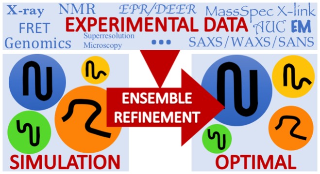
Ensemble refinement produces structural ensembles of flexible and dynamic biomolecules by integrating experimental data and molecular simulations. Here we present two efficient numerical methods to solve the computationally challenging maximum-entropy problem arising from a Bayesian formulation of ensemble refinement. Recasting the resulting constrained weight optimization problem into an unconstrained form enables the use of gradient-based algorithms. In two complementary formulations that differ in their dimensionality, we optimize either the log-weights directly or the generalized forces appearing in the explicit analytical form of the solution. We first demonstrate the robustness, accuracy, and efficiency of the two methods using synthetic data. We then use NMR J-couplings to reweight an all-atom molecular dynamics simulation ensemble of the disordered peptide Ala-5 simulated with the AMBER99SB*-ildn-q force field. After reweighting, we find a consistent increase in the population of the polyproline-II conformations and a decrease of α-helical-like conformations. Ensemble refinement makes it possible to infer detailed structural models for biomolecules exhibiting significant dynamics, such as intrinsically disordered proteins, by combining input from experiment and simulation in a balanced manner.

1. Introduction

To infer structures and functions of biological macromolecules, we combine information from diverse experimental and theoretical sources.¹⁻³ However, in many experiments the observables reporting on biomolecular structure are averaged over ensembles. Nuclear magnetic resonance (NMR) and pulsed electron paramagnetic resonance (EPR) experiments provide ensemble-averaged high-resolution information about distances (e.g., using the nuclear Overhauser effect, paramagnetic relaxation enhancement, or double electron–electron resonance (DEER))⁴⁻⁹ and angles (e.g., using J-couplings and residual dipolar couplings).^10,11 Small-angle X-ray scattering (SAXS) experiments provide ensemble-averaged information about macromolecular size and shape,¹² and wide-angle X-ray scattering (WAXS) experiments report on secondary structure and fold.¹³ Ensemble refinement promises faithful descriptions of the true ensemble of structures underlying the experimental data even for highly dynamic systems.^8,14−17

The conformational diversity of the ensemble can be described in terms of a set of representative reference structures. The relative weights of the ensemble members are then determined by ensemble refinement against experimental data. To regularize this inverse problem one can, for example, restrict the number of conformers as is done in minimal-ensemble refinement^8,18 or replica simulations,^15,19,20 limit the weight changes relative to the reference ensemble as is done in maximum-entropy approaches^14,15,21,22 or in Bayesian formulations,^4,21 or limit both ensemble size and weight changes.⁸ See ref (15) for an in-depth discussion and further references.

The reference ensemble is often defined in terms of a molecular simulation force field, that is, a classical potential energy function for which one has some confidence that it captures essential features. The experimental data can then be used directly as a bias in molecular dynamics (MD) simulations^5,19,23−28 or a posteriori to reweight an unbiased ensemble in a way that improves the agreement with experiment.^{8,18,21,29,30} Biased simulations improve the coverage of the configuration space but suffer from finite-size effects due to a limited ensemble size in simulations. Reweighting requires good coverage but can handle much larger ensemble sizes. The “Bayesian inference of ensembles” (BioEn) approach²¹ makes it possible to combine, if needed, biased sampling and subsequent reweighting to ensure both good coverage of the configuration space and a well-defined, converged ensemble.

Ensemble refinement by reweighting is a computationally challenging optimization problem because the number of structures in the ensemble, usually generated in simulations, and the number of experimental data points provided by experiments can both be large. Simulations can easily create hundreds of thousands of structures. In general, we would like to include as many structures as possible in ensemble refinement, not only to avoid artifacts due to the finite size of the ensemble²¹ but also to ensure that we pick up small but significant subensembles. Experiments like NMR, SAXS/WAXS, and DEER can provide thousands of data points. The numbers of pixels or voxels in electron-microscopy projection images or 3D maps, respectively, are of even larger magnitude. More than ten thousand data points are thus common when integrating data from different experimental sources.

With respect to computational efficiency, we also have to take into account that we usually want to perform multiple reweighting runs for different subensembles and subsets of the experimental data, while at the same time varying the confidence that we have in the reference ensemble. Consequently, we have to be able to efficiently solve the optimization problem underlying ensemble refinement by reweighting for large numbers of structures and data points.

The paper is organized as follows. In section 2, “Theory”, we present two complementary numerical methods to calculate the optimal ensemble by reweighting based on the “ensemble refinement of SAXS” (EROS) method,¹⁴ which is a special case of BioEn.²¹ In both methods, positivity and normalization constraints on the statistical weights are taken into account implicitly such that we can take advantage of efficient gradient-based optimization algorithms. In the first method, we solve for the logarithms of the N statistical weights, where N is the number of structures. In the second method, we solve for M generalized forces, where M is the number of experimental data points. The efficiency of the two methods depends on N and M. For both methods, we derive analytical expressions for the gradients that render gradient-based optimization algorithms highly efficient. In section 4, “Results”, we systematically investigate the efficiency and accuracy of these methods using synthetic data. For illustration, we then refine fully atomistic MD simulations of Ala-5 using J-couplings. In the Supporting Information, we present a detailed derivation of the gradients for correlated Gaussian errors.

2. Theory

We first present the BioEn posterior,²¹ whose maximum determines the optimal statistical weights of the structures in the ensemble. We then show that the optimal solution is unique. To be able to apply gradient-based optimization methods to the constrained optimization problem, we recast the posterior as a function of log-weights and as a function of the generalized forces, as already introduced in ref (21). For both formulations, we calculate the respective gradients analytically, facilitating efficient optimization. We focus here on uncorrelated Gaussian errors. Supporting Information contains a detailed derivation of the gradients for correlated Gaussian errors, which includes the expressions for uncorrelated Gaussians in the main text as special cases.

2.1. Background

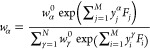
In the BioEn method,²¹ which is a generalization of the EROS method,¹⁴ we determine the optimum of the posterior probability as a function of the statistical weights, w_α, where α is the index of the N ensemble members (α = 1, ..., N) given the experimental data,

1

P(data|w) is the likelihood function, and w is the vector of weights w_α. The prior is given by

2

where

3

is the Kullback–Leibler divergence.³¹ Both refined weights (w_α > 0) and reference weights (w_α⁰ > 0) are normalized, ∑_α=1w_α = ∑_α=1^Nw_α = 1. The parameter θ expresses the confidence in the reference ensemble. Large values of θ express high confidence, and the optimal weights will be close to the reference weights.

Instead of maximizing the posterior with respect to w_α, we can minimize the negative log-posterior given by

4

The optimization problem is constrained by

5

and

6

that is, the weights lie in a simplex. For uncorrelated Gaussian errors, σ_i, of the ensemble-averaged measurements, Y_i, of the observables i = 1, ..., M, the likelihood is given by

7

Here, y_i^α is the calculated value of observable i for the individual structure α. Note that the measurements Y_i can stem from different experimental methods, for example, from SAXS and NMR, and that σ_i² = (σ_i,exp)² + (σ_i,calc)² is the sum of uncertainties in the experiment and in the calculation of the y_i.⁴

The negative log-posterior then becomes

8

Note that for Gaussian errors the negative log-posterior L corresponds to the EROS free energy χ² – θS, where S = −S_KL is the negative Kullback–Leibler divergence.¹⁴ The BioEn and EROS formulations differ by a factor 1/2 scaling χ², which is equivalent to a trivial rescaling of θ.

To solve this optimization problem efficiently, we first show that the negative log-posterior is convex such that there is a unique solution. The gradient of eq 8 is given by

9

where angular brackets indicate the average over the reweighted ensemble, that is, ⟨y_i⟩ = ∑_α=1^Nw_αy_i. The Hessian is given by

10

where δ_αγ = 1 if α = γ and δ_αγ = 0 otherwise. By casting the Hessian in this form, as a sum of a positive definite diagonal matrix and of dyadic products of vectors, it is straightforward to show that the quadratic form x^Thx is positive definite,

11

for |x|² = ∑_α=1^Nx_α² = 1. The Hessian is thus positive definite everywhere, and the optimal solution is unique.

A possible concern is that the optimal solution is on the boundary of the simplex, that is, w_α = 0 for some α, because the Kullback–Leibler divergence is bounded. One might then not be able to use gradient-based methods without modification. However, because of the nonanalytical character of the logarithm, the partial derivatives of L with respect to every w_α diverge to negative and positive infinity at w_α = 0 and 1, respectively, and are monotonic in between. Therefore, the optimal solution is contained within the simplex, not on its surface.

Another concern is that to find the unique optimal solution, we have to take into account the constraints acting on the weights given by eqs 5 and 6. One could optimize the log-posterior given by eq 8 using algorithms for constrained optimization like LBFGS-B that take advantage of the gradient.³² To avoid the performance penalty associated with treating constraints explicitly, we instead recast the optimization problem into an unconstrained form.

2.2. Optimization via Log-Weights

To optimize the log-posterior given by eq 8 under the constraints given by eqs 5 and 6 and to determine the optimal values of the weights w_α > 0 by gradient-based minimization, we introduce log-weights

12

which are only determined up to an additive constant. This constant cancels in the normalization of w_α. We can then write

13

Without loss of generality, because all w_α > 0, we can set g_N = 0. For the gradient of L with respect to the remaining g_μ (μ = 1, ..., N – 1), we have

14

where G_α = ln w_α⁰ and angular brackets indicate the average over the reweighted ensemble, for example, ⟨g⟩ = ∑_α=1w_αg_α. We simplified the expressions by taking advantage of the normalization condition.

Importantly, we need to minimize L only with respect to the N – 1 variables g_μ (μ = 1, ..., N – 1). A starting point of a gradient-based minimization of L could be the normalized prior w_α⁰, corresponding to g_α = ln(w_α/w_N⁰) = G_α – G_N. In a practical implementation, a procedure to evaluate L and its gradients, called with g_μ (μ = 1, ..., N – 1) as arguments, would do the following:

• (1)define g_N = 0,
• (2)evaluate w_α according to eq 13 for α = 1, ..., N,
• (3)evaluate L according to eq 8 or eq 17 below, and
• (4)evaluate the gradient according to eq 14.

Both L and its gradient can be evaluated efficiently using vector-matrix operations. Given the g_α, we define v_α = e^g_α, s = ∑_α=1^Nv_α = ∑_α=1e^g_α, s₀ = ∑_α=1^Ne^G_α, and w_α = v_α/s (all being efficiently evaluated in vector form). The averages can be calculated as vector dot products:

15

16

We then have

17

where ỹ is an M × N matrix with components ỹ_iα = y_i^α/σ_i, and Ỹ is a vector with M components Y_i/σ_i that can be precalculated.

To evaluate the gradient, the averages in eq 14 can be evaluated as dot products. The first part on the right-hand side of eq 14 can then be evaluated as an in-place vector operation. The second part can also be evaluated by a combination of matrix-vector multiplication (for ⟨y_i⟩), vector dot products (for the sum over i), and in-place vector operations (for the different μ).

2.3. Optimization via Generalized Forces

We showed previously²¹ that the weights at the maximum of the log-posterior can be expressed in terms of generalized forces

18

as

19

Note that these generalized forces correspond to Lagrange multipliers in closely related maximum entropy (MaxEnt) approaches to ensemble refinement.^{25,30,33−35} See ref (21) and the Discussion (section 5) below concerning the relation between MaxEnt and BioEn methods. In many practical cases, we have fewer observables than weights, M ≪ N. In such cases, one may want to take advantage of eq 19 and minimize L with respect to the M generalized forces F_k instead of the N weights. By applying the chain rule, we obtain the gradient with respect to the generalized forces as

20

In a numerical minimization of L with respect to the M generalized forces, one would thus at each iteration step do the following:

• (1)calculate the current weights w_α from the forces according to eq 19;
• (2)evaluate L according to eq 8 or eq 17;
• (3)evaluate the gradient according to eq 20.

Equations 8, 19, and 20 can be evaluated efficiently by using vector-matrix methods in NumPy etc., using precalculated vectors of intermediates. However, for large M × N, care should be taken to minimize the memory requirements by avoiding M × N matrices other than y_i^α.

2.4. Optimization Strategies

Small θ values are more challenging than large θ values because the optimal weights will deviate more from the reference weights. In practice, we usually do not know how to set θ a priori. In such cases, we recommend to perform an L-curve analysis.³⁶ In an L-curve or elbow plot, we plot χ² or the reduced chi-square value, χ²/M, as a function of the relative entropy S_KL for the optimal solutions at different θ values. The χ² values will decrease with increasing relative entropy S_KL, and we can choose a θ value corresponding to the elbow in this plot.

Finding optimal solutions for a series of θ values also has the advantage that we can use the more rapidly converging optimal solutions at large θ values as starting points for optimizations at smaller θ values.

3. Methods

3.1. Implementation

With the analytical expressions for gradients in the log-weights and forces formulations derived above, we can take advantage of highly optimized gradient-based optimization methods. The BioEn optimize package, which can be downloaded from https://github.com/bio-phys/BioEn, provides Python and C implementations of the log-posterior and its gradient for both methods and a selection of different gradient-based optimizers and implementations.

The reference implementation is based on Python and on the packages NumPy and SciPy in particular. The log-posterior and its derivatives are written in NumPy notation, and the BFGS minimizer from SciPy is used to compute the minimum.³⁷ Thanks to the fact that NumPy is typically linked to high-performance mathematical libraries such as MKL, the Python-based implementation is capable of exploiting vectorization and multithreading on state-of-the-art hardware. On the other hand, there is some overhead associated with NumPy related to the use of temporary buffers during expression evaluation.

To improve the performance, we provide C-based implementations of the log-posterior functions and their derivatives, largely avoiding temporary buffers by using explicit loops to implement the expressions. OpenMP directives are used to explicitly leverage vectorization and thread parallelization. The Python interfaces are written in Cython. While these kernels are significantly faster than the NumPy-based code, there is still some overhead when the BFGS minimizer from SciPy is used because it is written in plain Python.

To eliminate the bottleneck caused by the SciPy minimizer, we have implemented a Cython-based interface to the multidimensional minimizers of the GNU Scientific Library (GSL), that is, conjugate gradient, BFGS, and steepest descent minimizers.³⁸ In doing so, the minimization is performed completely in the C layer without any overhead from the Python layer. Additionally, the C implementation of Jorge Nocedal’s Fortran implementation of the limited-memory BFGS algorithm^39,40 by Naoaki Okazaki (https://github.com/chokkan/liblbfgs) can be used.

A test suite is provided to check the implementations against each other. During code development work, we noticed that performing parallel reductions can lead to numerically slightly different results. The reason is that parallel reductions introduce nondeterministic summation orders such that round-off errors vary between runs. Therefore, we also provide parallelized C kernels where we eliminated any nonreproducibility effects.

3.2. Simulation Details

Ala-5 was simulated at pH 2, using the AMBER99SB*-ildn-q force field matching the experimental solution conditions.⁴¹ To describe the protonated C-terminus at a low pH, we took partial charges from the protonated aspartate side chain. Excess charges were distributed across the C-terminal residue. The simulations of Ala-5 were run for 1 μs using simulation options previously described.⁴²J-couplings were calculated as in previous work⁴³ for the 50000 structures used for the BioEn reweighting. Chemical shifts were calculated with SPARTA+⁴⁴ using MDTraj.⁴⁵ MD simulations were analyzed using MDAnalysis.^46,47

4. Results

We first investigate the stability, accuracy, and efficiency of the optimization methods using log-weights and generalized forces by applying them to synthetic data. We then refine molecular dynamics simulation ensembles for Ala-5 using J-couplings.

4.1. Accuracy and Performance of Optimization Methods

We investigate how accuracy and efficiency of the log-weights and forces methods depend on the size of the ensemble N and the number of data points M using synthetic data. To generate a data set, we drew M experimental values Y_i from a normal distribution, that is, . We generated calculated observables y_iα by drawing Gaussian numbers from N(Y_i + 1, 2), where the offset of 1 mimics systematic deviations due to force field inaccuracies. We set the experimental error for all data points to σ = 0.5. For each combination of five M-values, M = 10², 316 (∼10^2.5), 10³, 3162 (∼10^3.5), and 10⁴, and nine N-values, N = 10², 316 (∼10^2.5), 10³, 3162 (∼10^3.5), 10⁴, 31623 (∼10^4.5), 10⁵, 316228 (∼10^5.5), and 10⁶, we generated randomly four sets, giving us 5 × 9 × 4 = 180 data sets in total.

To fully define the optimization problem, we chose uniform reference weights w_α⁰ = 1/N and a value for the confidence parameter θ = 0.01. The latter expresses little confidence in our reference ensemble, such that the optimal weights will be significantly different from the reference weights, rendering this optimization more challenging than for large values of θ. We minimize the negative log-posterior L given by eq 8 for each data set using the log-weights and forces methods.

The efficiency and accuracy of gradient-based optimization methods depends strongly on their detailed parametrization. Here, we present results for the limited-memory BFGS (LBFGS) algorithm.^39,40 Due to its memory efficiency, we can refine larger ensembles using more data points compared to other algorithms like BFGS or conjugate gradients. Specifically, we explored the effect of the choice of the line search algorithm and the convergence criteria on the convergence behavior. We found that using the backtracking line search algorithm applying the Wolfe condition^48,49 in connection with a convergence criterion acting on the relative difference of the log-posterior with respect to a previous value (relative difference 10 iterations before the current one <10^–6) strikes the best balance between accuracy, efficiency, and robustness. We used these parameters to obtain the results we show in the following. From all optimal solutions found in our exploration of the parameter space of the LBFGS algorithm, we chose for each data set the solution with the lowest negative log-posterior to compare with. We call these solutions the most optimal solutions in the following.

To characterize the optimization problem for the synthetic data sets considered here, we plot the optimal reduced χ² value as a function of the optimal relative entropies, S_KL, in Figure 1. The larger the value of the relative entropy S_KL, the more the optimal weights differ from the reference weights and the more challenging is the optimization problem. In general, we found that the optimal values for the log-weights and forces methods agree well with each other. Due to the nature of the synthetic data sets, results for individual (M, N) can be visually identified as clusters, especially for large ensemble sizes N. Note that for the data sets considered here, the clusters for large N pose more challenging optimization problems because the optimal weights are further from the initial weights.

Figure 1.

Scatter plot of the optimal reduced χ² and the optimal relative entropy, S_KL, obtained with the log-weights method (circles) and the forces method (crosses) for 5 × 9 = 45 values of (M, N) and θ = 0.01. For each value of (M, N), we show results for four synthetic data sets drawn at random as specified in the text. Crosses on top of circles indicate excellent agreement of the two methods. Optimal values for the four data sets for a specific (M, N) can be visually identified as clusters, especially for large N.

The optimal weights obtained with the two methods are highly correlated and correlate excellently with the most optimal weights found in our exploration of parameter space of the LBFGS algorithm. We quantify these correlations using Pearson’s correlation coefficient r,⁵⁰ which for two sets of weights w_α⁽¹⁾ and w_α is given by

21

We find that the cumulative distribution functions of the correlation coefficient for the forces and log-weights methods with respect to the most optimal weights found are strongly peaked at r = 1 (see Figure 2). For the forces method, 91% of all samples have a correlation coefficient of r > 0.99. For the log-weights method, the peak at r = 1 is even narrower as 95% of all samples have a correlation coefficient of r > 0.99. However, the log-weights solutions of fewer than 10 out of 180 samples have a correlation coefficient of r < 0.9 and thus show poorer correlation with the most optimal weights.

Figure 2.

Cumulative distribution functions of Pearson’s correlation coefficient r given by eq 21 of the optimized weights obtained with the log-weights and forces methods with respect to the most optimal weights found in optimizations with different parameters for the LBFGS algorithm. The lowest r values for particular (M, N) combinations are shown in Figure 3.

A more detailed analysis of the accuracy shows that the log-weights method performs not as well in cases where the ensemble size is much larger than the number of data points, N ≫ M. To quantify the accuracy, we calculate the difference in log-posterior, ΔL, obtained with the forces and log-weights methods to the most optimal negative log-posterior, L^(opt), found. An average over all samples for given M and N indicates that the forces method performs well (see Figure 3, top left). Only when M ≈ N, we find occasional small deviations from the most optimal values. The log-weights method performs excellently for M ≈ N, but not as well where N ≫ M. This behavior is also reflected in the minimum value of the correlation coefficients over the four random samples at given M and N (see Figure 3, bottom).

Figure 3.

Optimality of solutions as a function of the ensemble size N (horizontal axis) and number of experimental data points M (vertical axis) with respect to the most optimal solutions found with different convergence criteria and line search algorithms. (top) Difference of negative log-posterior values to optimum for the forces method (left) and the log-weights method (right). (bottom) Minimum value of the Pearson correlation coefficient r over the four samples at a given (M, N) with respect to the optimal weights for the forces method (left) and log-weights method (right).

For the chosen convergence criterion and line search algorithm, the log-weights method is computationally more efficient than the forces method (Figure 4). We performed benchmark calculations on a single node with two E5-2680-v3 CPUs, 12 cores each, and 64 GB RAM using OpenMP. For the largest system considered, (N, M) = (10⁶, 10⁵) we used a machine with identical CPUs but 128 GB RAM. For all values of the number of data points M, the run time as a function of the ensemble size N shows a step where the matrix of calculated observables y has reached a size of ∼10⁷ elements, that is, at M × N = 10² × 10⁵, 10³ × 10⁴, and 10⁴ × 10³. At this size, the matrix y no longer fits into the CPU cache. However, for larger sizes the run time again depends linearly on the ensemble size. In Table 1, we summarize the average run times for the largest ensemble size considered here (N = 10⁶). For M = 100 the log-weights methods is ∼20 times faster than the forces method (∼12 s versus ∼4 min on a single node; see Table 1).

Figure 4.

Run times for the log-weights (circles) and forces (crosses) optimization methods as a function of ensemble size N for different numbers of data points M = 100, 1000, and 10000 (in green, orange, and blue, respectively). Run times have been averaged (bold symbols) over four different synthetic data sets each (light symbols).

Table 1. Average Single-Node Run Time in Minutes and Minimum and Mean Value of the Pearson’s Correlation Coefficient, r, Calculated for the Optimized and Most Optimal Weights for the Largest Ensemble Size, N = 10⁶ and M = 100, 1000, and 10000 Data Points.

	run time [min]		min./avg. r
M	log-weights	forces	log-weights	forces
102	0.2	4	0.63/0.78	1.00/1.00
103	1.5	7	0.98/0.99	1.00/1.00
104	48	140	1.00/1.00	0.98/0.99

In conclusion, for the chosen convergence criterion and line search algorithm, optimization using the LBFGS algorithm is stable, efficient, and accurate for both the forces method and the log-weights method. In cases where the ensemble size is much larger than the number of data points, N ≫ M, the forces method is more accurate but also less efficient. In cases where N ≈ M, the log-weights method is both more efficient and more accurate than the forces method. The BioEn optimization library has been written to make it easy and straightforward not only to choose from a variety of optimization algorithms, but also to fine-tune the chosen optimization algorithms to further improve accuracy or efficiency or both.

4.2. Refinement of Ala-5 Using J-Couplings

As a realistic example for a biomolecular system, we have conducted BioEn refinement of the disordered peptide penta-alanine (Ala-5) against NMR J-couplings.⁴¹ The Ala-5 model system is simple enough that well converged simulations can be obtained straightforwardly. Nevertheless, it displays much of the complexity encountered in MD simulations of intrinsically disordered proteins (IDPs) with a myriad of shallow free energy minima. Hence, details of the force field matter greatly for such systems, and simulations do not provide results at a level routinely achieved for well-ordered proteins. NMR observables such as J-couplings, which report on dihedral angle equilibria, provide accurate information on disordered systems.⁵¹

We assessed the quality of a 1 μs simulation of Ala-5 with the AMBER99SB*-ildn-q force field by comparison to experimental J-couplings.⁴¹J-couplings were calculated from the MD trajectory using the Karplus parameters from the original publication⁴¹ and two sets of Karplus parameters determined from DFT calculations (DFT1 and DFT2).⁵² The DFT2 parameters were used to define the AMBER99SB*-ildn-q force field, and hence we initially focused on this set of Karplus parameters.

Even without refinement, the MD simulation gives very good agreement with the experimental J-couplings with χ²/M ≈ 1.0 (1.1 and 0.8 for original and DFT1 Karplus parameters, respectively) using the error model of ref (43). For uncorrelated errors, χ²/M < 1 would signify agreement within the experimental uncertainty on average. However, a closer inspection of measured and calculated J-couplings shows that there are systematic deviations. For the ³J_HNHα and ³J_HαC′ couplings, which report on the ϕ-dihedral angle equilibrium, the simulations predict larger couplings than in experiments (Figure 5A,C). In addition, for the ²J_NCα couplings, which are sensitive to the ψ-dihedral angle equilibrium, couplings calculated from simulations are all smaller than the experimental couplings (Figure 5G).

Figure 5.

Comparison of J-couplings measured by NMR⁴¹ (black squares) and calculated from MD simulation with the AMBER99SB*-ildn-q force field (red squares) and the optimal BioEn ensemble (blue circles, θ = 6.65). The DFT2 set of Karplus parameters was used to calculate J-couplings.

With BioEn reweighting, we refined the weights of 50000 structures from the 1 μs simulation of Ala-5 against 28 experimental J-couplings. Optimizing the effective log-posterior at different values of the confidence parameter θ (Figure 6A), we see the expected drop in χ² as θ is decreased. At small values of θ, we find only marginal improvements in χ², but start to move away from the reference weights as indicated by a substantial increase in the relative entropy. At θ = 6.65, we find a good compromise between reducing χ² and staying close to the reference weights. The agreement with experiment increased or stayed the same for all J-couplings (Figure S6) except for ³J_HNC′ and ³J_HNCβ of residue 2 for which the already very good agreement got somewhat worse (Supporting Information). The overall improvement demonstrates that the different experiments are consistent with each other. In particular, for the ³J_HNHα (Figure 5A) and ³J_HαC′ (Figure 5C) couplings, which report on the ϕ dihedral angle, and the ²J_NCα couplings (Figure 5G), reporting on the ψ dihedral angles, systematic deviations from the experiment disappear with the refinement. The changes in the weights are associated with an entropy S_KL ≈ 0.5 (Figure 6A). The weights of most structures were changed only slightly by the reweighting. In the optimal BioEn ensemble, the most important 20% of the structures constitute ∼60% of the refined ensemble (Figure 6B). The weights of these structures approximately double with the refinement. After refinement ∼20% of the structures contribute negligibly to the ensemble, with weights close to zero. As expected, the optimal weights from the log-weights or generalized forces methods were highly correlated (Figure S1), confirming the equivalence of the two methods to solve the BioEn reweighting problem. Using the LBFGS algorithm, the run times of the forces and log-weights optimizations for all θ values are comparable, at 42 and 33 s, respectively, on a standard workstation.

Figure 6.

BioEn optimization for Ala-5. (A) L-curve analysis to determine the optimal value of the confidence parameter θ by plotting χ² as a function of S_KL for different values of θ. (B) Cumulative weight of rank-ordered w_α for the uniformly distributed reference weights w_α⁰ (red) and for optimized weights (blue) at θ = 6.65 with S_KL ≈ 0.5.

The polyproline-II (ppII) conformation at ϕ ≈ −60° and ψ ≈ 150° becomes more populated in the optimal ensemble (Figure 7D), irrespective of the choice of Karplus parameters. The shift to ppII is in agreement with the original analysis of the J-couplings for Ala-5,⁴¹ where it was concluded that the ppII state dominates the conformational equilibrium, and with infrared (IR) spectroscopy.⁵³ The same conclusion was drawn from refining Ala-3 MD simulation ensembles against 2D-IR data.⁵⁴ The ³J_CC′ coupling for residue 2 has been highlighted as potentially spurious by Best et al.⁵⁵ because the reported coupling is atypical for a polyalanine. Leaving out this observable from the BioEn refinement results in an essentially unchanged refined ensemble (Figure S5). Using alternative Karplus parameters to calculate the J-couplings (Figure S2) also leads to a shift to the ppII state (original and DFT1 in Figures S3 and S4, respectively), and in all cases, the ppII state becomes more favorable at the expense of α-helical like conformations (Figure S5). For the original Karplus parameters, we also find a reduction in β-strand like conformations and an even larger ppII population than for DFT1 and DFT2. While the choice of Karplus parameter model somewhat affects the optimal ensemble, the overall conclusions are robust.

Figure 7.

Ala-5 Ramachandran maps. (A) Free energy surface G(ϕ,ψ) = −ln p(ϕ, ψ) from MD simulation with the AMBER99SB*-ildn-q force field averaged over the central residues 2–4. (B) Ramachandran plot for Ala residues outside of regular secondary structure from the PDB.¹¹ (C) Free energy surface for the optimal BioEn ensemble with DFT2 Karplus parameters. (D) Free energy differences between initial ensemble and the optimal BioEn ensemble.

The ensemble refinement improves and preserves the agreement with experimental data not included in the refinement, Protein Data Bank (PDB) statistics, and the experimental chemical shifts. The distribution of ϕ and ψ angles for Ala residues outside of regular secondary structure from the PDB,¹¹ while clearly not reflective of the structure of a specific disordered protein in solution, provides a measure of conformational preferences of disordered proteins. Indeed, the BioEn reweighting of the α and ppII conformations leads to a Ramachandran plot agreeing more closely with the PDB statistics, with a large reduction in the population of left-handed α-helical conformations as is apparent from Figure 7D, Figure S3, and Figure S4. No information from PDB statistics was included in the refinement and the improved agreement with an independent data set is encouraging. As a second independent data set, which was not included in the BioEn refinement, we compare the experimental chemical shifts for Ala-5⁴¹ to the initial ensemble and the optimal ensemble. The chemical shifts predicted by SPARTA+⁴⁴ are within the prediction error before and after ensemble refinement (Figure S7). The comparison shows the following for Ala-5: (1) Chemical shifts cannot be used to refine the ensemble because the initial ensemble already agrees with experiment within the large prediction error. (2) Ensemble refinement either improves or leaves unchanged predictions for observables not included in the refinement.

The BioEn reweighting leads to a better description of the disordered peptide Ala-5 and highlights the trade-offs inherent even in the most advanced force fields. Current fixed-charge protein force fields underestimate the cooperativity of the helix–coil equilibrium⁵⁶ because force fields describe the formation hydrogen bonds relatively poorly. To compensate for the lack of cooperativity of helix formation, the formation of α-helices was favored by the “star” correction to the ψ torsion potential with the aim to define a force field balanced between helix and coil conformations. The slight rebalancing of the AMBER force field⁵⁶ enabled the folding of both α-helical and β-sheet proteins.⁵⁷ Here BioEn reweighting compensates for an adverse effect of the overall very successful rebalancing of the AMBER force field, that is, the overestimation of the helix content for short peptides such as Ala-5. BioEn reweighting can thus serve as a system specific correction to the force field, which is a promising avenue to tackle systems such as intrinsically disordered proteins where the details of the force field are critical.^58,59

5. Discussion

We have presented two separate approaches to optimizing the BioEn posterior, the log-weights and generalized forces methods. Both approaches have in common that the resulting optimization problem is unconstrained, that is, both log-weights and forces can take on any real value in principle (with positivity of the weights enforced by the Kullback–Leibler divergence). For such unconstrained optimization problems, efficient gradient-based optimization methods exist. We take advantage of these by deriving analytical expressions for the gradients in both formulations.

The main differences between the log-weights and the forces methods concerns the dimensionality of the underlying optimization problem. Usually, higher-dimensional problems are harder to optimize. We can either optimize for N – 1 log-weights, where N is the ensemble size, or for M generalized forces, where M is the number of data points. We have shown here for the memory efficient LBFGS optimization algorithm^39,40 and synthetic data sets that optima corresponding to identical weights are reliably and efficiently found with both formulations.

Importantly, the BioEn method contains solutions of traditional MaxEnt approaches to ensemble refinement as special cases (see Figure 8). These methods either treat experimental observables as strict constraints^20,22,61,62 or consider errors explicitly.^25,30,60 If solutions for these methods exist then they correspond to different choices of the value of the confidence parameter θ: The BioEn optimal ensemble approaches the traditional MaxEnt solution with strict constraints forcing deviations from the experimental values to vanish, that is, χ² = 0, in the limit of θ → 0⁺. Note that if an experimental observable does not fall within the range of the calculated observables, such a strict constraint cannot be fulfilled and the MaxEnt method in principle fails to give a solution (though, in practice, methods such as replica sampling²⁰ will still give a result). In these cases where the MaxEnt solution does not exist, the limit of θ → 0⁺ corresponds to the least-χ² solution under the constraints that all weights are positive and normalized. As for MaxEnt approaches that account for Gaussian errors, the method of Cesari et al. gives the same solution as BioEn for θ = 1.^25,30 The MaxEnt method of Gull and Daniell⁶⁰ includes errors but uses a strict constraint by demanding that the reduced χ² is equal to one. If such a solution exists, then this condition determines a particular value of θ.

Figure 8.

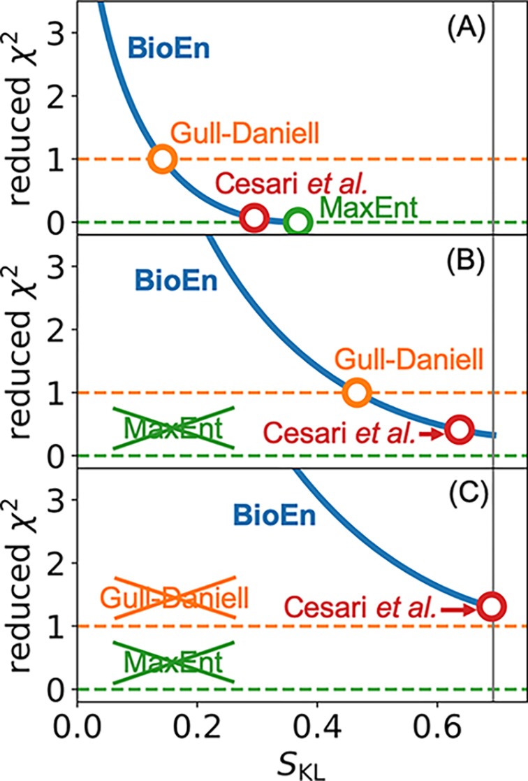
MaxEnt approaches to ensemble refinement as special cases of BioEn. For BioEn optimal ensembles, we plot the reduced χ² and the relative entropy S_KL parametrized by the confidence parameter θ (blue). The solution of Gull–Daniell-type⁶⁰ methods is given by the intersection of this curve with χ² = 1 (orange), of traditional MaxEnt methods^20,22,61,62 by the intersection with χ² = 0 (green), and of the method of Cesari et al.^25,30 by the BioEn solution for θ = 1 (red). For a simple model (M × N = 1 × 2, y = (0,1), σ = 0.14), we vary the experimental value Y, top to bottom. (A) All methods provide a solution for an experimental value Y = 0.09 within the range of calculated observables. (B) Traditional MaxEnt methods fail to give a solution for Y values outside this range (Y = 1.08). (C) Both traditional MaxEnt and Gull–Daniell-type methods fail to give a solution where a reduced χ² ≤ 1 cannot be realized by reweighting (Y = 1.16). The vertical gray lines indicate the maximum value S_KL = ln(2) for a two-state system.

Reweighting relies on good coverage of the conformational space such that the true ensemble underlying the experimental data is a subensemble of the simulation ensemble.⁶³ In coarse-grained simulations, sampling is efficient and the free-energy landscapes are smooth such that good coverage can be achieved. In atomistic simulations, where sampling is more expensive and the free energy landscape is rougher, we often have to apply enhanced sampling methods to obtain good coverage. Independent of the details of the enhanced sampling method and with or without steering by experimental values, one can use binless WHAM^42,64 or MBAR⁶⁵ to obtain the reference weights of the unbiased ensemble, which serve as input for ensemble refinement by reweighting.²¹

Here, we demonstrated that even without applying enhanced sampling methods, refinement of fully atomistic trajectories of penta-alanine using J-couplings alleviates deficiencies in the force field and leads to better agreement not only with the NMR data but also with expectations from experimental structures for proteins. These results indicate that ensemble refinement via reweighting is a promising route for highly flexible systems such as nucleic acids³⁰ and intrinsically disordered proteins.^58,59 For such systems, the number of accessible states can be enormous and consequently even small inaccuracies in the simulation force fields can lead to a poor representation of the experimental ensemble.

Importantly, ensembles do not have to be generated by simulations to be amenable to ensemble refinement via reweighting. For example, in the analysis of EPR experiments like DEER, libraries of the rotameric states of spin labels are used. For a specific residue, one selects from this library all rotameric states that do not have steric clashes with the protein structure. However, the interactions of the spin label with its surroundings can make some rotameric states in this ensemble more preferable than others. To account for this uncertainty, one can perform a BioEn refinement using the DEER data and the ensemble of rotameric states. This procedure has been used recently to resolve angstrom-scale protein domain movements.⁶⁶ BioEn-type ensemble refinement has also been applied successfully to IDP structural modeling using NMR data as input and coil libraries as reference.^10,11

To integrate experimental results, we often have to take nuisance parameters into account. For refining against SAXS intensities, we have to consider an unknown scaling parameter and often use an additive constant to account for inelastic scattering and, to a first approximation, for differences in the contrast. Using DEER data, we have to determine the modulation depths. We can include such nuisance parameters in the optimization either directly (by minimizing L simultaneously with respect to the weights and nuisance parameters) or iteratively. In the iterative approach, we perform the following: (1) A least chi-squared fit of the calculated ensemble averages determined by the current weights to the experimental data sets with the corresponding nuisance parameters as fit parameters. We have to perform one fit for every experimental method providing data. (2) With these fitted values of the nuisance parameters, we adjust the calculated observables y_i^α. These enter another round of optimization from which we obtain the optimal weights given the values of the nuisance parameters. (3) We use these weights for another round starting with step 1 until convergence is achieved. Note that instead of using least-chi-squared fits, one can also include priors acting on the nuisance parameters in both the direct and iterative formulations.

Interestingly, ensemble refinement by reweighting offers a way to quantify the agreement between simulations and experiment. After reweighting, we can make a quantitative statement of how much we would have had to change the simulated ensemble, expressed by the relative entropy or Kullback–Leibler divergence to be able to obtain agreement with experiment. The quantification of the agreement between simulation and experiment can also be used to identify and correct deficiencies in molecular dynamics force fields.²¹ In a perturbative formulation, one can seek force field corrections that capture the weight change.²⁵

BioEn accommodates a wide range of error models. With the gradients of the BioEn log-posterior presented here for Gaussian error models, with and without correlation, we already cover a large range of experimental methods. Moreover, in many cases the Gaussian error model can be used to efficiently obtain an initial estimate for the optimal weights. These estimates can then be used as initial weights for an optimization using a more accurate error model but perhaps a less efficient optimization method. We provide an open-source implementation at https://github.com/bio-phys/BioEn at no cost under the GPLv3 license.

Supporting Information Available

The Supporting Information is available free of charge on the ACS Publications website at DOI: 10.1021/acs.jctc.8b01231.

• Detailed derivation of the gradients for correlated Gaussian errors, which includes the expressions for uncorrelated Gaussian in the main text as special cases, comparison of the Ala-5 ensemble refinement using generalized forces and log-weights, quantification of the effects of the choice of Karplus parameters on the optimal Ala-5 ensemble, discussion of the information content of individual J-couplings, and comparison of calculated chemical shifts to experiment (PDF)

We acknowledge financial support from the German Research Foundation (CRC902: Molecular Principles of RNA Based Regulation) and by the Max Planck Society.

The authors declare no competing financial interest.

References

- Ward A. B.; Sali A.; Wilson I. A. Integrative Structural Biology. Science 2013, 339, 913–915. 10.1126/science.1228565. [DOI] [PMC free article] [PubMed] [Google Scholar]
- Bottaro S.; Lindorff-Larsen K. Biophysical experiments and biomolecular simulations: A perfect match?. Science 2018, 361, 355–360. 10.1126/science.aat4010. [DOI] [PubMed] [Google Scholar]
- Bonomi M.; et al. Principles of protein structural ensemble determination. Curr. Opin. Struct. Biol. 2017, 42, 106–116. 10.1016/j.sbi.2016.12.004. [DOI] [PubMed] [Google Scholar]
- Rieping W.; Habeck M.; Nilges M. Inferential Structure Determination. Science 2005, 309, 303–306. 10.1126/science.1110428. [DOI] [PubMed] [Google Scholar]
- Scheek R. M.; et al. Structure Determination by NMR. The Modeling of NMR Parameters As Ensemble Averages. NATO Advanced Science Institutes Series Series A Life Sciences 1991, 225, 209–217. 10.1007/978-1-4757-9794-7_15. [DOI] [Google Scholar]
- Lange O. F.; et al. Recognition Dynamics up to Microseconds Revealed from an RDC-Derived Ubiquitin Ensemble in Solution. Science 2008, 320, 1471–1475. 10.1126/science.1157092. [DOI] [PubMed] [Google Scholar]
- Olsson S.; et al. Probabilistic Determination of Native State Ensembles of Proteins. J. Chem. Theory Comput. 2014, 10, 3484–3491. 10.1021/ct5001236. [DOI] [PubMed] [Google Scholar]
- Boura E.; et al. Solution Structure of the ESCRT-I Complex by Small-Angle X-Ray Scattering EPR and FRET Spectroscopy. Proc. Natl. Acad. Sci. U. S. A. 2011, 108, 9437–9442. 10.1073/pnas.1101763108. [DOI] [PMC free article] [PubMed] [Google Scholar]
- Boura E.; et al. Solution Structure of the ESCRT-I and -II Supercomplex Implications for Membrane Budding and Scission. Structure 2012, 20, 874–886. 10.1016/j.str.2012.03.008. [DOI] [PMC free article] [PubMed] [Google Scholar]
- Mantsyzov A. B.; et al. A maximum entropy approach to the study of residue-specific backbone angle distributions in α-synuclein, an intrinsically disordered protein. Protein Sci. 2014, 23, 1275–1290. 10.1002/pro.2511. [DOI] [PMC free article] [PubMed] [Google Scholar]
- Mantsyzov A. B.; et al. MERA: a webserver for evaluating backbone torsion angle distributions in dynamic and disordered proteins from NMR data. J. Biomol. NMR 2015, 63, 85. 10.1007/s10858-015-9971-2. [DOI] [PMC free article] [PubMed] [Google Scholar]
- Koch M. H. J.; Vachette P.; Svergun D. I. Small-angle scattering: a view on the properties, structures and structural changes of biological macromolecules in solution. Q. Rev. Biophys. 2003, 36, 147–227. 10.1017/S0033583503003871. [DOI] [PubMed] [Google Scholar]
- Makowski L.; et al. Characterization of Protein Fold by Wide-Angle X-ray Solution Scattering. J. Mol. Biol. 2008, 383, 731–744. 10.1016/j.jmb.2008.08.038. [DOI] [PubMed] [Google Scholar]
- Rozycki B.; Kim Y. C.; Hummer G. SAXS Ensemble Refinement of ESCRT-III Chmp3 Conformational Transitions. Structure 2011, 19, 109–116. 10.1016/j.str.2010.10.006. [DOI] [PMC free article] [PubMed] [Google Scholar]
- Boomsma W.; Ferkinghoff-Borg J.; Lindorff-Larsen K. Combining Experiments and Simulations Using the Maximum Entropy Principle. PLoS Comput. Biol. 2014, 10, e1003406 10.1371/journal.pcbi.1003406. [DOI] [PMC free article] [PubMed] [Google Scholar]
- Sali A.; et al. Outcome of the First wwPDB Hybrid/Integrative Methods Task Force Workshop. Structure 2015, 23, 1156–1167. 10.1016/j.str.2015.05.013. [DOI] [PMC free article] [PubMed] [Google Scholar]
- Vallat B.; et al. Development of a Prototype System for Archiving Integrative/Hybrid Structure Models of Biological Macromolecules. Structure 2018, 26, 894. 10.1016/j.str.2018.03.011. [DOI] [PMC free article] [PubMed] [Google Scholar]
- Berlin K.; et al. Recovering a Representative Conformational Ensemble from Underdetermined Macromolecular Structural Data. J. Am. Chem. Soc. 2013, 135, 16595–16609. 10.1021/ja4083717. [DOI] [PMC free article] [PubMed] [Google Scholar]
- Best R. B.; Vendruscolo M. Determination of Protein Structures Consistent with NMR Order Parameters. J. Am. Chem. Soc. 2004, 126, 8090–8091. 10.1021/ja0396955. [DOI] [PubMed] [Google Scholar]
- Roux B.; Weare J. On the Statistical Equivalence of Restrained-Ensemble Simulations With the Maximum Entropy Method. J. Chem. Phys. 2013, 138, 084107. 10.1063/1.4792208. [DOI] [PMC free article] [PubMed] [Google Scholar]
- Hummer G.; Köfinger J. Bayesian ensemble refinement by replica simulations and reweighting. J. Chem. Phys. 2015, 143, 243150. 10.1063/1.4937786. [DOI] [PubMed] [Google Scholar]
- Pitera J. W.; Chodera J. D. On the Use of Experimental Observations to Bias Simulated Ensembles. J. Chem. Theory Comput. 2012, 8, 3445–3451. 10.1021/ct300112v. [DOI] [PubMed] [Google Scholar]
- White A. D.; Voth G. A. Efficient and Minimal Method to Bias Molecular Simulations with Experimental Data. J. Chem. Theory Comput. 2014, 10, 3023–3030. 10.1021/ct500320c. [DOI] [PubMed] [Google Scholar]
- White A. D.; Dama J. F.; Voth G. A. Designing Free Energy Surfaces That Match Experimental Data With Metadynamics. J. Chem. Theory Comput. 2015, 11, 2451–2460. 10.1021/acs.jctc.5b00178. [DOI] [PubMed] [Google Scholar]
- Cesari A.; Gil-Ley A.; Bussi G. Combining Simulations and Solution Experiments as a Paradigm for RNA Force Field Refinement. J. Chem. Theory Comput. 2016, 12, 6192–6200. 10.1021/acs.jctc.6b00944. [DOI] [PubMed] [Google Scholar]
- Dannenhoffer-Lafage T.; White A. D.; Voth G. A. A Direct Method for Incorporating Experimental Data into Multiscale Coarse-Grained Models. J. Chem. Theory Comput. 2016, 12, 2144–2153. 10.1021/acs.jctc.6b00043. [DOI] [PubMed] [Google Scholar]
- Bonomi M.; et al. Metainference: A Bayesian inference method for heterogeneous systems. Sci. Adv. 2016, 2, e1501177 10.1126/sciadv.1501177. [DOI] [PMC free article] [PubMed] [Google Scholar]
- Bonomi M.; Camilloni C.; Vendruscolo M. Metadynamic metainference: Enhanced sampling of the metainference ensemble using metadynamics. Sci. Rep. 2016, 6, 31232. 10.1038/srep31232. [DOI] [PMC free article] [PubMed] [Google Scholar]
- Francis D. M.; et al. Structural basis of p38 alpha regulation by hematopoietic tyrosine phosphatase. Nat. Chem. Biol. 2011, 7, 916–924. 10.1038/nchembio.707. [DOI] [PMC free article] [PubMed] [Google Scholar]
- Bottaro S.; et al. Conformational ensembles of RNA oligonucleotides from integrating NMR and molecular simulations. Sci. Adv. 2018, 4, eaar8521 10.1126/sciadv.aar8521. [DOI] [PMC free article] [PubMed] [Google Scholar]
- Kullback S.; Leibler R. A. On Information and Sufficiency. Ann. Math. Stat. 1951, 22, 79–86. 10.1214/aoms/1177729694. [DOI] [Google Scholar]
- Byrd R. H.; Nocedal J.; et al. A Limited Memory Algorithm for Bound Constrained Optimization. SIAM Journal on Scientific and Statistical Computing 1995, 16, 1190–1208. 10.1137/0916069. [DOI] [Google Scholar]
- Mead L. R.; Papanicolaou N. Maximum entropy in the problem of moments. J. Math. Phys. 1984, 25, 2404–2417. 10.1063/1.526446. [DOI] [Google Scholar]
- Cesari A.; Reißer S.; Bussi G. Using the Maximum Entropy Principle to Combine Simulations and Solution Experiments. Computation 2018, 6, 15. 10.3390/computation6010015. [DOI] [Google Scholar]
- Bottaro S.; Bengtsen T.; Lindorff-Larsen K.. Integrating Molecular Simulation and Experimental Data: A Bayesian/Maximum Entropy Reweighting Approach. Preprint bioRxiv, https://www.biorxiv.org/content/10.1101/457952v1, 2018. [DOI] [PubMed]
- Hansen P. C.; O’Leary D. P. The Use of the L-Curve in the Regularization of Discrete Ill-Posed Problems. SIAM J. Sci. Comput. 1993, 14, 1487–1503. 10.1137/0914086. [DOI] [Google Scholar]
- Fletcher R.Practical Methods of Optimization, 2nd ed.; Wiley-Interscience: New York, NY, USA, 1987. [Google Scholar]
- Nocedal J.; Wright S. J.. Numerical Optimization, 2nd ed.; Springer: New York, 2006. [Google Scholar]
- Liu D. C.; Nocedal J. On the limited memory BFGS method for large scale optimization. Math. Program. 1989, 45, 503–528. 10.1007/BF01589116. [DOI] [Google Scholar]
- Nocedal J. Updating Quasi-Newton Matrices with Limited Storage. Math. Comput. 1980, 35, 773–782. 10.1090/S0025-5718-1980-0572855-7. [DOI] [Google Scholar]
- Graf J.; et al. Structure and Dynamics of the Homologous Series of Alanine Peptides: A Joint Molecular Dynamics/NMR Study. J. Am. Chem. Soc. 2007, 129, 1179–1189. 10.1021/ja0660406. [DOI] [PubMed] [Google Scholar]
- Stelzl L. S.; et al. Dynamic Histogram Analysis To Determine Free Energies and Rates from Biased Simulations. J. Chem. Theory Comput. 2017, 13, 6328–6342. 10.1021/acs.jctc.7b00373. [DOI] [PubMed] [Google Scholar]
- Best R. B.; Buchete N.-V.; Hummer G. Are Current Molecular Dynamics Force Fields too Helical?. Biophys. J. 2008, 95, L07–L09. 10.1529/biophysj.108.132696. [DOI] [PMC free article] [PubMed] [Google Scholar]
- Shen Y.; Bax A. SPARTA+: a modest improvement in empirical NMR chemical shift prediction by means of an artificial neural network. J. Biomol. NMR 2010, 48, 13–22. 10.1007/s10858-010-9433-9. [DOI] [PMC free article] [PubMed] [Google Scholar]
- McGibbon R. T.; et al. MDTraj: A Modern Open Library for the Analysis of Molecular Dynamics Trajectories. Biophys. J. 2015, 109, 1528–1532. 10.1016/j.bpj.2015.08.015. [DOI] [PMC free article] [PubMed] [Google Scholar]
- Michaud-Agrawal N.; et al. MDAnalysis: A Toolkit for the Analysis of Molecular Dynamics Simulations. J. Comput. Chem. 2011, 32, 2319–2327. 10.1002/jcc.21787. [DOI] [PMC free article] [PubMed] [Google Scholar]
- Gowers R. J.; et al. MDAnalysis: A Python Package for the Rapid Analysis of Molecular Dynamics Simulations. Proceedings of the 15th Python in Science Conference 2016, 98–105. 10.25080/Majora-629e541a-00e. [DOI] [Google Scholar]
- Wolfe P. Convergence Conditions for Ascent Methods. SIAM Rev. 1969, 11, 226–235. 10.1137/1011036. [DOI] [Google Scholar]
- Wolfe P. Convergence Conditions for Ascent Methods. II: Some Corrections. SIAM Rev. 1971, 13, 185–188. 10.1137/1013035. [DOI] [Google Scholar]
- Pearson K. Notes on regression and inheritance in the case of two parents. Proc. R. Soc. London 1895, 58, 240–242. 10.1098/rspl.1895.0041. [DOI] [Google Scholar]
- Meier S.; Blackledge M.; Grzesiek S. Conformational distributions of unfolded polypeptides from novel NMR techniques. J. Chem. Phys. 2008, 128, 052204. 10.1063/1.2838167. [DOI] [PubMed] [Google Scholar]
- Case D. A.; Scheurer C.; Brüschweiler R. Static and Dynamic Effects on Vicinal Scalar J Couplings in Proteins and Peptides: A MD/DFT Analysis. J. Am. Chem. Soc. 2000, 122, 10390–10397. 10.1021/ja001798p. [DOI] [Google Scholar]
- Feng Y.; et al. Structure of Penta-Alanine Investigated by Two-Dimensional Infrared Spectroscopy and Molecular Dynamics Simulation. J. Phys. Chem. B 2016, 120, 5325–5339. 10.1021/acs.jpcb.6b02608. [DOI] [PMC free article] [PubMed] [Google Scholar]
- Feng C.-J.; Dhayalan B.; Tokmakoff A. Refinement of Peptide Conformational Ensembles by 2D IR Spectroscopy: Application to Ala-Ala-Ala. Biophys. J. 2018, 114, 2820–2832. 10.1016/j.bpj.2018.05.003. [DOI] [PMC free article] [PubMed] [Google Scholar]
- Best R. B.; Zheng W.; Mittal J. Balanced Protein-Water Interactions Improve Properties of Disordered Proteins and Non-Specific Protein Association. J. Chem. Theory Comput. 2014, 10, 5113–5124. 10.1021/ct500569b. [DOI] [PMC free article] [PubMed] [Google Scholar]
- Best R. B.; Hummer G. Optimized Molecular Dynamics Force Fields Applied to the Helix-Coil Transition of Polypeptides. J. Phys. Chem. B 2009, 113, 9004–9015. 10.1021/jp901540t. [DOI] [PMC free article] [PubMed] [Google Scholar]
- Lindorff-Larsen K.; et al. Systematic Validation of Protein Force Fields against Experimental Data. PLoS One 2012, 7, e32131. 10.1371/journal.pone.0032131. [DOI] [PMC free article] [PubMed] [Google Scholar]
- Wright P. E.; Dyson H. J. Intrinsically disordered proteins in cellular signalling and regulation. Nat. Rev. Mol. Cell Biol. 2015, 16, 18. 10.1038/nrm3920. [DOI] [PMC free article] [PubMed] [Google Scholar]
- Fisher C. K.; Stultz C. M. Constructing ensembles for intrinsically disordered proteins. Curr. Opin. Struct. Biol. 2011, 21, 426–431. 10.1016/j.sbi.2011.04.001. [DOI] [PMC free article] [PubMed] [Google Scholar]
- Gull S. F.; Daniell G. J. Image-Reconstruction from Incomplete and Noisy Data. Nature 1978, 272, 686–690. 10.1038/272686a0. [DOI] [Google Scholar]
- Cavalli A.; Camilloni C.; Vendruscolo M. Molecular Dynamics Simulations With Replica-Averaged Structural Restraints Generate Structural Ensembles According to the Maximum Entropy Principle. J. Chem. Phys. 2013, 138, 094112. 10.1063/1.4793625. [DOI] [PubMed] [Google Scholar]
- Boomsma W.; et al. Equilibrium Simulations of Proteins Using Molecular Fragment Replacement and NMR Chemical Shifts. Proc. Natl. Acad. Sci. U. S. A. 2014, 111, 13852–13857. 10.1073/pnas.1404948111. [DOI] [PMC free article] [PubMed] [Google Scholar]
- Rangan R.; et al. Determination of Structural Ensembles of Proteins: Restraining vs Reweighting. J. Chem. Theory Comput. 2018, 14, 6632. 10.1021/acs.jctc.8b00738. [DOI] [PubMed] [Google Scholar]
- Rosta E.; et al. Catalytic Mechanism of RNA Backbone Cleavage by Ribonuclease H from Quantum Mechanics/Molecular Mechanics Simulations. J. Am. Chem. Soc. 2011, 133, 8934–8941. 10.1021/ja200173a. [DOI] [PMC free article] [PubMed] [Google Scholar]
- Shirts M. R.; Chodera J. D. Statistically optimal analysis of samples from multiple equilibrium states. J. Chem. Phys. 2008, 129, 124105. 10.1063/1.2978177. [DOI] [PMC free article] [PubMed] [Google Scholar]
- Reichel K.; et al. Precision DEER Distances from Spin-Label Ensemble Refinement. J. Phys. Chem. Lett. 2018, 9, 5748–5752. 10.1021/acs.jpclett.8b02439. [DOI] [PubMed] [Google Scholar]
Associated Data
This section collects any data citations, data availability statements, or supplementary materials included in this article.