

Abstract
Stimulation of the suppressive surround of a cortical neuron affects the responsivity and tuning of the classical receptive field (CRF) on several stimulus dimensions. In V1 and V2 of macaques prepared for acute electrophysiological experiments, we explored the chromatic sensitivity of the surround and its influence on the chromatic tuning of the CRF. We studied receptive fields of single neurons with patches of drifting grating of optimal spatial frequency and orientation and variable size, modulated along achromatic or isoluminant color directions. The responses of most neurons declined as the patch was enlarged beyond the optimal size (surround suppression). In V1 the suppression evoked by isoluminant gratings was less than one-half that evoked by achromatic gratings. Consequently, many cells were most sensitive to achromatic modulation when patches just covered the CRF but were most sensitive to isoluminant modulation when patches were enlarged to cover the suppressive surround. Non-oriented neurons that were strongly chromatically opponent generally lacked suppressive surrounds. In V2 most neurons showed equal surround suppression from isoluminant gratings and achromatic gratings. This makes the relative sensitivity of V2 neurons to achromatic and isoluminant gratings mainly independent of the size of the grating. We also measured the chromatic properties of the CRF in the presence of differently colored surrounds. In neither V1 nor V2 did the surround alter the chromatic tuning of the CRF. Cortical mechanisms sensitive to chromatic contrast seem to provide little input to the suppressive surrounds of V1 neurons but substantial input to those of V2 neurons.
Keywords: extrastriate, suppression, color, receptive field, striate cortex, vision
Introduction
The color of a surface depends substantially on the context in which it appears. Dramatic shifts in color appearance can be brought about by embedding a target in either a uniformly colored (Walraven, 1976; Shevell, 1978) or patterned (Singer and D'Zmura, 1994; Monnier and Shevell, 2003) surround. These phenomena might be relevant to the preservation of surface appearance in the face of changes in the chromaticity of illumination (color constancy), and possible mechanisms underlying them have been sought in several cortical areas (Zeki, 1983a,b; Desimone et al., 1985; Schein and Desimone, 1990; Moutoussis and Zeki, 2002; Wachtler et al., 2003). Two known mechanisms within receptive fields might make cortical cells sensitive to chromatic context. First, within the classical receptive field (CRF), the region in which contrast variations directly affect the discharge, chromatic context could affect neuronal responses by activating spatially distinct regions that receive cone-opponent inputs of opposite sign (“double-opponency”) (Livingstone and Hubel, 1984; Thorell et al., 1984; Conway, 2001; Johnson et al., 2001). Second, chromatic context could affect neuronal responses through the otherwise silent region surrounding the CRF, where stimuli cause no response when presented alone but alter the response when the CRF also is stimulated, generally via suppression (Blakemore and Tobin, 1972; Maffei and Fiorentini, 1976; Levitt and Lund, 1997). This suppressive surround usually is tuned for orientation and spatial frequency and often for direction of movement; the visual stimulus that elicits the greatest response from the CRF is also the one that induces the greatest suppression from the surround (DeAngelis et al., 1992; Levitt and Lund, 1997; Cavanaugh et al., 2002b). Although the suppressive surround has been implicated previously in chromatic contextual interactions (Ts'o and Gilbert, 1988; Wachtler et al., 2003), no study has characterized the relationship between the chromatic preference of the CRF and the region surrounding it or the nature of the interactions between the two regions.
One aim of the present work is to characterize the chromatic properties of the suppressive surround of receptive fields in V1 and V2 and to show how, if at all, the surround affects the chromatic tuning of the CRF. Given the potential for surround influence, a second aim is to understand how the size of the stimulus falling on the receptive field influences the overall chromatic selectivity of a cell [in most earlier work that used sinusoidal gratings (Thorell et al., 1984; Lennie et al., 1990), the chromatic properties of cortical neurons have been characterized with large patches of gratings]. We investigate both V1 and V2 because several reports (Levitt et al., 1994; Kiper et al., 1997) point to quantitative differences between the chromatic properties of cells in these areas. We used comparable stimuli in the two areas so that we could establish whether there were differences in the chromatic properties of surrounds.
We show that in V1 the suppressive surround is relatively insensitive to chromatic contrast, preferring instead achromatic contrast, and that its preferred chromaticity is correlated poorly with that of the CRF. This results in many neurons being substantially more sensitive to chromatic contrast when excited by large stimuli than when excited by stimuli confined to the CRF. Neurons in V2 behave differently. The preferred chromaticity of the surround is well correlated with that of the CRF, and the surround therefore acts to suppress the response to large areas that have the same chromatic structure.
Materials and Methods
Preparation and recording. Experiments were undertaken on nine adult male macaque monkeys (8 Macaca fascicularis and 1 Macaca radiata) weighing between 3.75 and 5.5 kg. Each animal initially was anesthetized with ketamine hydrochloride (Vetalar, 10 mg/kg, i.m.). The saphenous veins were cannulated, and surgery was continued under thiopental sodium anesthesia. The monkey was intubated, the head placed in a stereotaxic frame, and a craniotomy made over the occipital cortex, centered on or near the lunate sulcus. Electrodes were attached to the skull to monitor the electroencephalogram (EEG) and to the forearms and legs to monitor the electrocardiogram (ECG). All procedures conformed to the guidelines approved by the New York University Animal Welfare Committee.
Postsurgical anesthesia was maintained by continuous infusion of sufentanil citrate (4-12 μg/kg per hr) in physiological solution (Normosol-R, Abbott Laboratories, North Chicago, IL) with added dextrose (2.5%). Then muscular paralysis was induced and maintained by continuous infusion of vecuronium bromide (100 mg/kg per hr). The monkey was respirated artificially so as to keep end-tidal CO2 near 33 mmHg. The EEG and ECG were monitored continuously, and at any sign of the anesthesia becoming less effective the dose of sufentanil citrate was increased. Rectal temperature was kept near 37°C with the use of a heating blanket.
The pupils were dilated with atropine sulfate (typically to 7 mm), and the corneas were protected with high-permeability contact lenses that remained in place for the duration of the experiment. No artificial pupils were used. Supplementary lenses (with power determined by ophthalmoscopy) were used to focus the eyes at a distance of 114 cm. At the beginning of the experiment, and at regular intervals afterward, the positions of the foveae were mapped by reverse ophthalmoscopy.
A small incision was made in the dura, and a guide tube containing the electrode (Ainsworth tungsten-in-glass or paralyene-coated tungsten, FHC, 1-5 mΩ) was positioned over this. The guide tube was aligned approximately normally or tangentially to the cortical surface, depending on the target cortical area. In nine normal penetrations we began in V1 and then passed through white matter into V2. In six tangential penetrations we recorded only in V1. In all penetrations the receptive fields were located between 2 and 5° from the fovea. The dura was covered with warm agar and sealed with dental acrylic. The analog signal from the electrode was amplified, filtered, and sampled at 11.025 or 22.05 kHz by a dual processor Power Macintosh computer. Putative spikes were displayed on a monitor, and templates for discriminating spikes were constructed by averaging multiple traces. The timing of waveforms that matched the template was recorded with an accuracy of 0.1 msec. Electrolytic lesions (3-5 μA for 3-5 sec) were made at points along the track to allow later reconstruction. At the end of the experiment the monkey was given 60 mg/kg sodium pentobarbitone (Nembutal) and then perfused transcardially with 0.9% saline in 0.1 m phosphate buffer (PB), followed by a solution of 10% formalin in PB and then 10% sucrose in PB. The brain was blocked and transferred to 30% sucrose until it sunk. Parasagittal sections (50 μm) were cut on a freezing microtome and stained for Nissl substance or reacted for cytochrome oxidase (Wong-Riley, 1979). Electrode tracks were reconstructed from the positions of the lesions made during the experiment. Our use of parasagittal sections maximized the lengths of recovered electrode tracks, but made it impossible for us to identify their locations in the “thin” or “thick” cytochrome oxidase stripes in V2.
Visual stimuli. Sinusoidal gratings were generated by the same computer that recorded spikes and were displayed on a calibrated monitor (Sony G500, Tokyo, Japan), refreshed at 90 Hz, and viewed from 114 cm. Multiple independently controlled gratings could be displayed simultaneously and were drawn by using commands to OpenGL. Each grating was presented within a circular window or annulus with hard edges. The remainder of the screen was held at the mean luminance of ∼50 cd/m2 (CIE 1931 x, y ∼0.30, 0.32). All stimuli were defined by spatiotemporal modulation around this point. These modulations can be represented in a three-dimensional color space as described previously (Derrington et al., 1984; Lennie et al., 1990). Along the L-M axis only the signals from L- and M-cones vary, in opposition, without variation in luminance. Along the orthogonal S-cone isolating axis there is no modulation of either the L- or M-cones. The L-M and S axes define a plane in which only chromaticity varies. Normal to this plane is the achromatic axis along which the signals from all three cone classes vary in proportion. Figure 1 shows this color space.
Figure 1.

Color space used to specify stimuli. The space is defined by three axes: an L-M axis in which the signals of the L- and M-cones covary to keep their sum constant, an S-cone isolating axis, and an achromatic axis in which the signals of the three cone classes vary in proportion. The L-M and S-cone axes define an isoluminant plane in which chromaticity varies without a change in luminance. In this plane stimuli are specified by their azimuth relative to the L-M axis, where an azimuth of 0° is +(L-M) modulation. In the two other principal planes of the color space (that formed by the L-M and achromatic axes and that formed by the S-cone and achromatic axes) stimuli are specified by their elevation from the isoluminant plane (0°). Stimuli modulated along the achromatic axis have an elevation of 90°. For this study stimuli in the L-M/achromatic plane had an azimuth of 0°, and stimuli in the S-cone/achromatic plane had an azimuth of 90°.
In all of the experiments the stimuli are grating patterns, or spatially uniform fields, defined by modulation along some vector through the white point in this space. The direction of the vector is defined by two angles: the elevation (the angle to the isoluminant plane, where 90° is the normal) and the azimuth (the angle within the isoluminant plane, where 0° represents +L-M modulation and 90° -S modulation). The maximum attainable modulation along the achromatic axis produced a Michelson contrast:
 |
of 1.0 for each cone class. Full modulation along the L-M axis gave cone contrasts of 0.08 for the L-cones, 0.15 for the M-cones, and 0.001 for the S-cones. Full modulation along the S-axis produced contrasts of 0.85 for the S-cones and <0.002 for the L- and M-cones. In many of the experiments described below we compare the effectiveness of achromatic gratings modulated along different directions in color space. There is no universally agreed metric for comparing the responsiveness of neurons to modulation along different directions (Brainard, 1996). Our aim was always to work with modulation amplitudes that elicited well driven responses of below-saturating amplitude and that were of approximately equal size for different directions of modulation. In separate experiments we established that full modulation along the isoluminant axes always elicited responses of below-saturating amplitude and that in most neurons these responses were comparable to ones elicited by an achromatic contrast of 0.2. We used this contrast routinely. Our choice has the added advantage of permitting comparison with previous work (Johnson et al., 2001).
For each cell we determined the preferred orientation, then the preferred spatial frequency, and then the preferred temporal frequency with the use of small (usually 1-2° in diameter) patches of drifting grating. The position of the receptive field was determined by using a smaller (0.1-0.2° diameter) grating patch under manual control. For experiments that used central and annular grating patches, the orientation, direction, spatial, and temporal frequency of the two gratings were identical. When measurements were made, the stimuli in a set (one of which was always was a blank screen) were presented in random order, each 10-20 times, in trials lasting 2 sec. Between each trial the screen was blank (at the mean luminance) for 0.5 sec.
Data analysis. From the train of impulses discharged during each stimulus presentation, we extracted the mean rate and the amplitude of the Fourier component at the frequency of stimulation. Cells were identified as simple if the amplitude of the fundamental Fourier harmonic exceeded the elevation in mean firing rate (Skottun et al., 1991).
We used a ratio-of-Gaussians function to model interactions between the CRF and suppressive surround. It has the form:
 |
1 |
where erf is the error function, x is the diameter of the grating patch, and the free parameters are Se and Ke, the size and sensitivity of the CRF Gaussian; Si and Ki, the size and sensitivity of the suppressive Gaussian, and the exponent n. R0 is the measured spontaneous activity of the cell. Here the sizes Se and Si refer to the diameter of the Gaussian at 1/e times the peak sensitivity. The exponent was constrained to be between 1 and 5, and the space constant of the surround was constrained to be greater than that of the CRF.
To determine the preferred color direction of a cell, as well as the weights assigned to different cone classes, we fit a linear model to cell responsivity measured along several directions in color space. Modulation depths along isoluminant color directions were always the maximum available; modulation depths outside the isoluminant plane were chosen to generate response levels that were robust but remained below saturating response levels. If a cell combines cone signals linearly and responds in proportion to this combined signal, then the amplitude of response to any color direction (vector) is given by the dot product of the stimulus vector and the vector that describes the preferred color direction of the cell, such that:
 |
2 |
where R is responsivity [impulses(imp)/sec per unit contrast], K is a scale factor, θ and ϕ are the elevation and azimuth of the stimulus vector, and θm and ϕm are the elevation and azimuth of the preferred color direction vector of the cell. R0 is the spontaneous activity of the cell. The sign of the response to a particular direction of modulation is given by the response phase. For a complex cell this information is unavailable, and so we use a full-wave rectified version of the linear model:
 |
3 |
The parameters are the same as for Equation 2. Some cells showed sharper tuning in this color space than is predicted by the cosine function of Equation 2. In these cases the best fits were obtained by adjusting the model slightly such that response resulted from passing the signal through an expansive nonlinearity (Kiper et al., 1997; De Valois et al., 2000). We therefore used this adjusted model for all cells, constraining the exponent of the expansive nonlinearity to be between 1 and 5.
The preferred elevation and azimuth provide a convenient indication of the chromatic signature of a cell, but a deeper expression of it is represented by the weights the cell assigns to the modulated signals from each of the cone classes: wL, wM, and wS. These can be derived from the preferred color directions of Equations 2 or 3 (Lennie et al., 1990). We obtain the relative weights assigned to the cone classes by dividing each cone weight by the sum of the absolute weights attached to all three cone classes, yielding:
 |
4 |
for the L-cone weight and equivalent functions for the other cones.
For each model we express the quality of fit as the percentage of response variance that the model accounted for. We first calculated the mean response across trials for each stimulus (R). We then calculated the mean response across stimuli (Rs). The mean square distance between the response to each stimulus and the mean response is the response variance:
 |
5 |
The difference between the model prediction for each stimulus (Rm) and the response of the cell (R) can be determined by substituting Rm for Rs in Equation 5. We call the resultant value Vmodel. Then the percentage of variance that the model accounts for is defined as:
 |
6 |
If the model predicts the response perfectly, it will account for 100% of the variance. Best-fitting solutions to the models were found by minimizing the mean square error between the prediction and the data, using the constr function of the Optimization Toolbox for MatLab (v5.2, MathWorks, Natick, MA).
Results
Simple and complex cells were not distinguished by their expression of surround effects and are not separated in what follows. Among cells that lacked orientation selectivity, those that were strongly chromatically opponent were distinctive in some respects and are discussed separately when this was the case.
Size tuning for different color directions
CRF-surround interactions become apparent when the length, width, or diameter of a stimulus grows from a size smaller than the CRF to encroach progressively on the suppressive surround. We characterized these interactions by measuring size-tuning curves for patches of drifting gratings that were modulated along each of three color directions: achromatic, L-M, or S-cone isolating (Fig. 1). Along each chromatic axis the modulation was the maximum attainable; along the achromatic axis the contrast was set to 0.2, high enough to ensure that most neurons responded well but low enough that these responses were seldom saturated (see Materials and Methods). Gratings were of optimal orientation and spatial and temporal frequency, and they moved in the preferred direction for the CRF.
Figure 2 shows examples of size-tuning curves obtained from five V1 cells and two V2 cells. For some cells in V1 and most cells in V2 the curves that were obtained in different color directions were scaled versions of each other (Fig. 2A,E). For many V1 cells, however, the shapes of size-tuning curves varied with color direction (Fig. 2B-D). To characterize these effects for our population of cells, we measured the preferred size and degree of surround suppression for each cell that responded with >10 imp/sec to modulation along at least one chromatic axis. Individual tuning curves were analyzed if the cell responded with at least 5 imp/sec to that color direction. To characterize the difference between the peak response and that obtained in the largest aperture, we calculated a surround suppression index (SI):
 |
where Resp is the difference between the baseline firing rate and the stimulus-driven firing rate (Cavanaugh et al., 2002a).
Figure 2.

Size-tuning curves for achromatic and chromatic gratings. A, V1 simple cell preferring L-M modulation and showing no surround suppression for either achromatic or chromatic gratings (spatial frequency for all gratings, 0.7 cyc/°). B, V1 simple cell showing a change in preferred color direction in larger grating patches (0.9 cyc/°). C, V1 simple cell showing increased color responsivity in larger grating patches but maintaining a preference for achromatic modulation (1 cyc/°). D, V1 complex cell preferring achromatic modulation in small patches and L-M modulation in large patches (1.6 cyc/°). E, V2 complex cell showing surround suppression for each color direction (0.6 cyc/°). F, Comparison of surround suppression for two cells that responded only to L-M modulation. The V1 simple cell shows some suppression in large patches (0.4 cyc/°). The V2 simple cell shows complete suppression (0.6 cyc/°). The smooth curves in each panel are the best-fitting solutions to a ratio-of-Gaussians model described in Materials and Methods. Horizontal lines show the spontaneous firing rates. Error bars are ±1 SEM.
Table 1 and Figures 3 and 4 show the results of this analysis. For achromatic gratings the average preferred diameter was 0.86° in V1 and 1.27° in V2 (Fig. 3A,C). Extending the grating patch beyond this size revealed surround suppression in most cells, with a median surround suppression of 54% in V1 and 71% in V2 (Fig. 4A,C). For stimuli modulated along either of the chromatic axes, the preferred patch size was usually larger and surround suppression was observed in fewer cells (Table 1). This was particularly so in V1, where median surround suppression was 27% for L-M gratings and 21% for S-cone gratings (Fig. 4A). In V2 a greater proportion of cells showed surround suppression for chromatic stimuli: median surround suppression was 47% for L-M gratings and 62% for S-cone gratings (Fig. 4C).
Table 1.
Descriptive parameters obtained from size-tuning curves in V1 and V2
|
|
V1 |
V2 |
|---|---|---|
| Cells responding to achromatic modulation | 137 | 66 |
| Average diameter at peaka | 0.86 | 1.27 |
| Median suppression (SI) | 54% | 71% |
| Number of cells suppressedb | 109 (80%) | 53 (80%) |
| Cells responding to L-M modulation | 121 | 57 |
| Average diameter at peaka | 1.20 | 1.79 |
| Median suppression (SI) | 27% | 47% |
| Number of cells suppressedb | 62 (51%) | 39 (68%) |
| Cells responding to S-cone modulation | 78 | 48 |
| Average diameter at peaka | 1.61 | 1.47 |
| Median suppression (SI) | 21% | 62% |
| Number of cells suppressedb | 36 (46%) | 38 (79%) |
| Total cells |
150 |
68 |
Geometric mean.
More than 25% suppression (SI).
Figure 3.

Dependence of preferred patch size on color direction. A, C, Diameter of the patch generating the largest response for each color direction in V1 (A) and V2 (C). Top row, Achromatic gratings; middle row, L-M gratings; bottom row, S-cone isolating gratings. Arrow above each distribution indicates the average preferred size (see Results). B, D, Comparison of preferred sizes for modulation along different color directions in V1 (B) and V2 (D). Parameters in A-D were derived only from tuning curves that exceeded a criterion of 5 imp/sec. Dashed lines in B and D are lines of unity.
Figure 4.

Influence of color direction on magnitude of surround suppression. Same format as Figure 3. A, C, Percentage of surround suppression (SI) for each color direction in V1 (A) and V2 (C). Top row, Achromatic gratings; middle row, L-M gratings; bottom row, S-cone isolating gratings. B, D, Comparison of surround suppression for different color directions in V1 (B) and V2 (D). Parameters were derived only from tuning curves that exceeded a criterion of 5 imp/sec. Dashed lines in B and D are lines of unity.
Figures 3, B and D, and 4, B and D, compare the preferred sizes and amounts of surround suppression elicited by stimuli modulated along different directions in color space. Among V1 neurons the preferred size measured with achromatic gratings was almost always smaller than that measured with chromatic gratings, and there was little correlation between the two measurements (Fig. 3B,D). Among V2 neurons the preferred sizes were more similar for chromatic and achromatic gratings. Corresponding relationships held for degree of suppression by the surround (Fig. 4). In V1 the neurons were more suppressed by achromatic gratings than by chromatic ones, and there was little correlation between the two measurements. In V2 the neurons were suppressed more equally by achromatic and chromatic gratings.
Approximately 15% of neurons (24 in V1 and 9 in V2) clearly preferred chromatic modulation over achromatic modulation and thus showed approximately balanced opponent cone inputs to the CRF (Fig. 2A,F). These cells usually lacked orientation specificity and responded well to spatially uniform fields. When such cells responded to achromatic gratings, these gratings elicited a moderate degree of surround suppression (V1, median SI = 47%, n = 13; V2, SI = 53%, n = 7). On the other hand, chromatic gratings rarely evoked surround suppression in V1 (L-M, SI = 0%, n = 22; S-cone, SI = 0%, n = 17) but evoked substantial surround suppression in some V2 cells (L-M, SI = 54%, n = 8; S-cone, SI = 68%, n = 6).
In summary, isoluminant gratings elicited little surround suppression in V1, so the shapes of the size-tuning curves of many cells thus depended on color direction. This suggests that the suppressive surrounds of most V1 cells prefer achromatic stimuli. V2 behaved differently: isoluminant gratings could elicit substantial surround suppression in V2, and the shapes of size-tuning curves did not depend on color direction.
A receptive field that incorporates chromatic sensitivity
We found that many V1 cells that were equally responsive to isoluminant and achromatic gratings when tested with large patches were far more responsive to achromatic than isoluminant gratings when tested with smaller patch sizes. Thus the suppressive surround was relatively more sensitive to achromatic stimuli than was the CRF. This same property also might explain why preferred size increases when isoluminant gratings are used: the less potent signal from the surround allows more of the CRF to be exposed (Cavanaugh et al., 2002a). To characterize the sensitivity of CRF and surround to stimuli modulated along different color directions, we have explored a model of CRF-surround interactions in which the surround acts divisively to normalize the CRF response (Sceniak et al., 2001; Cavanaugh et al., 2002a). In the following we show that this model describes size-tuning curves obtained along different color directions, and we use it to determine the chromatic sensitivity of the CRF and the surround.
Our implementation of the ratio-of-Gaussians model (Eq. 1) uses one Gaussian spatial envelope to describe the CRF and another to describe the suppressive surround mechanism (for details, see Materials and Methods). The surround acts divisively on the CRF response, and the resultant output is passed through an expansive nonlinearity. In fitting the model to size-tuning curves (multiple curves were fit concurrently), we allowed the sensitivities of the CRF and surround Gaussians to vary with color direction, but we kept the space constants of the Gaussians and the exponent of the expansive nonlinearity constant. The contrast of each grating is not explicit in the model but is absorbed into the sensitivity terms.
The smooth curves in Figure 2 are the best-fitting predictions of the model. The model copes naturally with the color dependence of preferred size by adjusting the relative sensitivities of the CRF and surround to different color directions. The model predicts that the low chromatic sensitivity of many V1 surrounds leads to a larger preferred size for chromatic gratings as the full size of the CRF is unveiled (Fig. 2B) (see also Cavanaugh et al., 2002a). This inherent flexibility in the model meant that it captured well the shapes of all of the size-tuning curves we observed. To illustrate this, we determined the quality of fits quantitatively as the proportion of variance in response that it accounts for (see Materials and Methods). For the cells in Figure 2 the model accounted for an average 95.6% of the variance (range, 91.2-98.9%). Across the whole population of cells the model accounted, on average, for 93.1% of the variance in the data (SD 8.8; n = 218). For the cells that responded to all three color directions, the model accounted for 94.5% (SD 7.0; n = 106) of the variance.
Another indication of the value of the model is the plausibility of the parameters returned by the best-fitting solutions. In V1 neurons the geometric mean diameter (at 1/e times the peak sensitivity) of the CRF was 0.94° (n = 150) and of the surround was 2.97° (n = 120). Estimates of surround size were included only if surround suppression (SI) was at least 25% in one or more color directions. (Fig. 6 shows the distributions of these values.) The estimate of CRF size is very similar to that found in other recent studies (Sceniak et al., 2001; Angelucci et al., 2002; Cavanaugh et al., 2002a); the average surround diameter is somewhat larger. The differences between studies are generally small, and we conclude that our estimates are within reasonable bounds. Among V2 neurons the average sizes of the CRF (1.40°; n = 68) and surround (5.42°; n = 59) were ∼1.5 times those of neurons in V1 (see Fig. 7). To our knowledge, no other estimates exist for V2.
Figure 6.

Distributions of CRF and surround sizes in V1 for cells of different color sensitivity. Sizes were estimated by concurrently fitting a ratio-of-Gaussians model to size-tuning curves in different color directions. A, B, Sizes of CRF (A) and surrounds (B) of neurons that were much more sensitive to achromatic modulation than to isoluminant modulation. C, D, Sizes of CRF (C) and surrounds (D) that were approximately equally sensitive to chromatic modulation and achromatic modulation. E, F, Sizes of CRF (E) and surrounds (F) that were more sensitive to L-M modulation or S-cone modulation than to achromatic modulation. The arrows show the geometric means for each group (open arrows) and all cells (filled arrows), the values of which are as follows. CRF: all, 0.94, n = 150; achromatic, 1.02, n = 73; intermediate, 0.72, n = 57; isoluminant, 1.53, n = 20. Surround: 2.97, n = 100; 3.28, n = 64; 1.97, n = 24; 2.31, n = 12.
Figure 7.

Distributions of CRF and surround sizes in V2 for cells of different color sensitivity. Sizes were estimated by concurrently fitting a ratio-of-Gaussians model to size-tuning curves in different color directions. Same format is used as for Figure 6. The arrows show the geometric means for each group (open arrows) and all cells (filled arrows), the values of which are as follows. CRF: all, 1.4, n = 68; achromatic, 1.59, n = 25; intermediate, 1.27, n = 38; isoluminant, 1.54, n = 5. Surround: 5.42, n = 53; 4.79, n = 25; 4.75, n = 22; 8.43, n = 6.
Because the space constants of both CRF and surround are fixed in the model, the relative responsivity of CRF or surround to gratings in different color directions is controlled only by the sensitivity terms. The relative responsivity of the CRF to isoluminant gratings (i.e., the ratio of chromatic to achromatic responsivity) therefore can be calculated as:
 |
for L-M gratings and similarly for S-cone isolating gratings. The same calculations can be made for the surround.
We first asked whether the relative chromatic responsivities of CRF and surround were related. To make this comparison, we plotted the relative chromatic sensitivity (Z1) of the CRF against that of the surround. In this case the cells that responded to only one color direction or showed little surround suppression (<25%) for any color direction were excluded. Figure 5 shows that for most cells in V1 the relative chromatic sensitivity of the surround was less than that of the CRF (points lie below the diagonal lines in Fig. 5A,B). However, for most cells in V2 the relative chromatic sensitivity of the CRF and surround was similar, and most points clustered around the diagonal line.
Figure 5.

Comparison of relative chromatic responsivity of CRF and suppressive surround in V1 and V2. The responsivity of CRF and surround to modulation along each color direction was obtained from size-tuning curves as described in Results. The relative chromatic responsivity of CRF or surround, calculated as described in Results, is the L-M/achromatic ratio (A), the S-cone/achromatic ratio (B), or the L-M/S-cone ratio (C). A, Relative responsivity to L-M and achromatic gratings in surround versus CRF. Dashed line is the unity line. Histogram in the bottom panel is the ratio of the surround index on CRF index. Open bars and open circles represent V1 cells; stippled bars and filled circles represent V2 cells. The bars displaced to the right of the histogram include cells with a ratio >10 and cells in which the surround was completely unresponsive to L-M modulation (surround L-M/achromatic ratio = 0). B, Relative responsivity to S-cone isolating and achromatic gratings in surround versus CRF. Same format as A. Bars displaced to the right of the histogram include cells with a ratio >10 and cells in which the surround was completely unresponsive to S-cone modulation. C, Relative responsivity to L-M and S-cone isolating gratings in surround versus CRF. Same format as A and B.
We can estimate the chromatic selectivity of both CRF and surround as the ratio of the relevant L-M and S-cone sensitivity terms. In Figure 5C we plot this ratio for the CRF against that for the surround. In both V1 and V2 the cells cluster around the diagonal line, although more tightly in V2. This suggests that, when the surround is sensitive to chromatic modulation, the relative weight of S-cone and L-M mechanisms is similar to that of the CRF. In V1 a number of surrounds showed less sensitivity to S-cone modulation than the CRF. This was not the case in V2.
We then asked whether the degree of chromatic sensitivity in CRF and surround mechanisms varied with mechanism size. For this analysis we used parameter Z1 to sort CRFs into three mutually exclusive groups: those that preferred achromatic gratings (Z1 < 0.5 for L-M and Z1 < 0.5 for S-cone), those for which the responsivities to chromatic and achromatic directions were approximately equal (0.5 ≤ Z1 < 2 for L-M and/or 0.5 ≤ Z1 < 2 for S-cone), and those that preferred chromatic gratings (Z1 ≥ 2 for L-M and/or Z1 ≥ 2 for S-cone). If a cell responded to only one color direction, its CRF was categorized as either preferring achromatic or isoluminant gratings. We sorted surrounds in the same way except that we excluded cells that responded to only one color direction or showed little surround suppression for any color direction. These groups help us reveal interesting patterns in data, but their boundaries are arbitrary; we do not believe that they distinguish classes of cells. Johnson et al. (2001) use similar categories to distinguish cells in their sample and found approximately the same proportions.
Figure 6 compares the distribution of CRF and surround sizes for each group within V1. The CRF mechanism of one-half of the cells in V1 (73 of 150, 49%) was far more responsive to achromatic gratings than to either chromatic grating. These cells show a broad distribution of CRF size (Fig. 6A). The CRF mechanism of 20 cells (13%) was more responsive to one or both chromatic gratings than achromatic. These cells were usually non-oriented, had low-pass spatial frequency tuning, and generally showed slightly larger CRF sizes than cells preferring achromatic stimuli (Fig. 5E). Finally, the center mechanism of 57 cells (38%) was approximately equally responsive to chromatic and achromatic gratings. The CRF sizes of these cells were the smallest that were encountered (Fig. 6C). Figure 6, B, D, and E, shows the counterpart relationships for the surround. Most V1 surrounds were far more sensitive to achromatic gratings than chromatic ones (64 of 100; Fig. 6B). Twelve cells (12%; Fig. 6F) had surrounds that preferred chromatic gratings, and 24 (24%; Fig. 6D) cells had surrounds that were equally responsive to chromatic and achromatic. Figure 7 shows the corresponding comparisons for cells in V2. The CRF mechanisms of 25 of 68 cells (37%) and the surround mechanisms of 25 of 53 cells (47%) were more responsive to achromatic than chromatic gratings, smaller proportions than the corresponding ones in V1. As for V1, V2 CRFs that were approximately equally sensitive to chromatic and achromatic gratings were among the smallest we encountered. We found no variation in surround size with chromatic sensitivity.
Color sensitivity of surround suppression
Because surround suppression appears to act divisively, it is observable only if the CRF is active. Since the chromaticity of the stimulus on the CRF and the surround never differed, the low chromatic sensitivity of the CRF of many cells might have led us to underestimate the prevalence and strength of chromatic inputs to the surround. We therefore explored the chromatic sensitivity of the suppressive surround by using central and annular grating patches for which the color directions could be varied independently. The color direction of the central patch was set to the preferred color direction for the CRF (usually achromatic) at a contrast that gave robust responses below saturating response levels. Both grating patches had the same spatial frequency, orientation, and direction of movement. The inner diameter of the annulus was set to the smallest that evoked no response when the annulus was presented alone. The advantage of this stimulus configuration is that surround activity can be studied under constant levels of excitation to the CRF. One disadvantage is that, because CRF and surround regions usually overlap, the annulus grating will not cover the potent inner portion of the surround. We made measurements on 70 of the cells previously described and an additional 13 V2 cells, altogether 50 V1 cells and 33 V2 cells. We used annuli modulated along each of nine directions in the three principal planes of our color space (Fig. 1; see Materials and Methods). The modulation depth along each chromatic axis was always the maximum available. The stimulus set also included achromatic annuli of contrast 0.2.
Figure 8 shows the responses of each of three cells to the central patch of grating presented alone, to the annulus presented alone, and the central patch presented in the presence of the annulus. For each cell the responses are plotted as a function of the color direction of the annulus. The three graphs in each column show the amplitudes of responses to the set of color directions in three principal planes. Figure 8A shows the behavior of a V1 complex cell in which the grating on the CRF was achromatic. For this cell, only achromatic gratings in the surround suppressed the response. Figure 8B shows the behavior of a V1 simple cell for which the CRF preferred isoluminant gratings. When the CRF was stimulated by an isoluminant central grating, no annulus suppressed the response. The size tuning of this cell is illustrated in Figure 2B. The V2 simple cell in Figure 8C also preferred isoluminant gratings on the CRF, but unlike the V1 cell its response was suppressed substantially by the annular grating and more so by isoluminant than by achromatic annuli. Its size tuning is illustrated in Fig. 2F.
Figure 8.

Color tuning of surround suppression. Each column shows the set of responses obtained from one cell driven by a small patch of grating presented by itself (dashed line) or together with annular gratings modulated in different color directions (filled symbols). Responses are plotted against the color direction of the annular grating. The color direction of the small patch is constant and is indicated by the arrow in each column. Open symbols show responses to annular gratings presented alone. Each row shows results obtained with the annulus modulated in a different plane in color space (top row, isoluminant plane; middle row, plane formed by the L-M and achromatic axes; bottom row, plane formed by the S-cone and achromatic axes). A, V1 complex cell that preferred achromatic gratings and showed no suppression from isoluminant annuli (spatial frequency, 2 cyc/°; inner diameter of annulus, 1°). B, Simple cell in V1 that preferred isoluminant gratings and showed no suppression from annuli of any color direction (0.9 cyc/°; 2°). C, Simple cell in V2 that preferred isoluminant gratings and was more suppressed by gratings of a similar chromatic composition than by any other grating (0.6 cyc/°; 1.4°). Open squares are the suppression induced by achromatic gratings of contrast 0.2. Error bars are ± 1 SEM.
To summarize the results of these experiments, we calculated an index of the suppression brought about by the annulus:
 |
This is essentially the same as the index used to summarize size-tuning curves. Figure 9A-C shows pairwise comparisons of suppression induced by annuli along each of the cardinal color directions. Annuli modulated in isoluminant color directions induced little suppression; in V1 the L-M annuli generated an average of 5.1% suppression and the S-cone annuli generated 5.7% suppression (n = 50). Isoluminant annuli were slightly more suppressive in V2: L-M, 9.6%; S-cone, 12.5%; n = 33. Achromatic annuli of low contrast (0.2) induced more suppression than chromatic annuli (V1, 17.1%; V2, 37.1%); increasing annulus contrast to 1 increased the suppression, but not in proportion to the change in contrast [Fig. 9D; a linear regression had a slope of 1.03 rather than 5 (data not shown)]. All of these estimates of surround suppression are lower than those obtained with size-varying grating patches (Fig. 4). We compared for individual cells the estimates of surround suppression obtained under the two conditions (Figs. 2B, 8C). Cells suppressed by annuli modulated in a particular color direction usually showed surround suppression for size tuning in that direction. The converse was not the case: many cells showed surround suppression for size tuning, but not for annuli.
Figure 9.

Comparison of surround suppression obtained by using achromatic and chromatic (isoluminant) annuli. A, Suppression by L-M gratings and achromatic annuli of contrast 0.2. B, Suppression by S-cone annuli and achromatic annuli of contrast 0.2. C, Suppression by L-M annuli and S-cone annuli. D, Suppression by achromatic annuli of low contrast (0.2) and achromatic annuli of high contrast (1). Values <0 indicate enhancement of response rather than suppression. Dashed lines in A-D are lines of unity.
The relatively weak suppression brought about by annuli (compared with enlargement of grating patches) is consistent with overlapping center and surround mechanisms (Cavanaugh et al., 2002a). Our requirement that no annulus produce an excitatory response from a cell could place the annulus outside the most potent region of the surround. Surround suppression was particularly hard to generate with isoluminant annuli, indicating that chromatic mechanisms in the surround either are localized close to the CRF or did not reach threshold when stimulated with an annulus.
Cone inputs to cells measured for small and large fields
The relative sensitivity of a cell to chromatic and achromatic gratings often is used to determine whether cone inputs to a cell are opponent or non-opponent. Our results bear on this because we have shown that size tuning curves obtained with achromatic and chromatic patterns often differ enough to cause the relative chromatic sensitivity of V1 cells to change with patch size (Fig. 2B,D). Among 148 V1 cells on which we studied size tuning, 29 preferred the L-M stimulus to an achromatic when stimulated with the patch size optimal for achromatic gratings; 54 preferred the L-M grating when larger patches were used (16 cells did not respond at all to large patches). As might be expected from Figures 1, 2, 3, changing patch size had less effect on V2 neurons; when patches were of optimal size, 15 of 67 cells preferred L-M modulation; when patches were large, 16 cells (of 50 that responded to large patches) preferred L-M modulation. We therefore explored fully the chromatic tuning of neurons when they were stimulated by small patches of grating (the preferred size when achromatic) and by large ones (diameter, 6-8°).
Figure 10 shows, in the format used in Figure 8, the responses of three cells to modulation along nine directions in the principal planes of color space, measured by using both small and large grating patches. The color directions are the same as those used previously for annuli, but the modulation depth along each direction was adjusted to ensure that responses were below saturating levels. We assume that within this range of firing rates the cell responses are approximately proportional to the modulation of cone inputs, and we therefore plot cell responsivity (imp/sec per unit contrast).
Figure 10.

Responsivity to different color directions for small and large patches of grating. Each column shows the responsivity (imp/sec per unit contrast) of one cell to gratings modulated along vectors in each of the three principal planes of the color space (top row, isoluminant plane; middle row, the plane formed by the L-M and achromatic axes; bottom row, the plane formed by the S-cone and achromatic axes). A, V1 simple cell that prefers achromatic modulation. Extension of the grating patch reduces responsivity to all color directions. Note the different scale in the top panel (responsivity calculated from the F1 modulated rate; spatial frequency, 2 cyc/°; diameter of small patch, 0.5°). B, V1 simple cell that prefers chromatic modulation. Extension of the grating patch causes little change in firing rate for any color direction (responsivity calculated from the F1; 0.6 cyc/°; 0.8°). C, V2 simple cell that prefers chromatic modulation. Extension of the grating patch reduces responsivity to each color direction (responsivity calculated from the F1; 0.5 cyc/°; 1.4°). Continuous lines are the best-fitting solutions of a linear model described in Materials and Methods.
The V1 cell in Figure 10A showed low responsivity to isoluminant gratings in both small and large patches; its responsivity to achromatic and intermediate color modulation was high for small patches and negligible for large ones. The V1 cell in Figure 10B preferred isoluminant stimuli in both small and large patch sizes; its responsivity was unaffected by patch size. The V2 cell in Figure 10C also preferred isoluminant gratings in both small and large patches, but responsivity in all color directions was lower for larger patches.
To characterize the measurements, we fit the curves obtained from simple cells with a linear model of cone summation (Eq. 2) (Derrington et al., 1984) and an expansive output nonlinearity. For complex cells we used a full-wave rectified version of that model (Eq. 3) (Lennie et al., 1990), again with the output nonlinearity. The best-fitting solutions are shown as smooth curves in Figure 10. We fit measurements from 112 cells (87 in V1 and 25 in V2) that provided criterion response levels for at least one color direction for both small and large grating patches. For V1 cells the model accounted for 90.0% of the variance in small patches and 84.1% in large patches (see Materials and Methods). For V2 cells the model accounted for 86.7% of the variance in small patches and 84.1% in large patches. The changes in chromatic signature brought about by changing patch size were in many cells large and reliable. To check the reliability of estimates, we fit the model separately to data from each trial of the stimulus set and then analyzed the resulting sets of preferred color directions as distributions on a unit sphere (Mardia, 1972). By the criterion that the two distributions of preferred color directions differ at the 0.05 level, 27 V1 cells (31%) and five V2 cells (20%) had different preferred directions for small and large patches.
We derived the relative weights and signs of cone inputs to receptive fields from their preferred color directions (see Materials and Methods). Figure 11 shows these distributions of cone weights for each neuron. The estimates obtained for small and large fields are linked by lines. The absolute signs of L- and M-cone input cannot be recovered from these measurements (Johnson, 2001), so in Figure 11 we have adopted the following convention: cells with L- and M-cone inputs of opposite sign are shown as having negative L-cone weights (points to the left of the midline), and cells with L- and M-cone inputs of the same sign are shown as having positive L-cone weights (points to the right of the midline). Cells that receive no S-cone input are represented by points on the diagonals. The greater the S-cone input to a cell, the further inside the diagonal its point will lie.
Figure 11.

Relative weights attached to the inputs from each cone type, measured by using small and large patches of grating in V1 and V2. A, V1 cells. B, V2 cells. For cells that responded only to small patches of grating, only the cone weights measured with the small patch are shown (large open symbols). For other cells a line connects the measurements made with the small patch (small open symbol) and the large patch (filled symbol).
Figure 11 shows that changing the size of the stimulating patch could alter substantially the relative weights of cone inputs to the receptive field. This happened mainly for cells that showed no cone opponency for small patch sizes (open circles, in the right half of each panel); cells that showed well balanced opponent L- and M-cone inputs (near the midpoint on the left diagonal) or substantial S-cone input (far from the diagonal) usually showed little change in relative cone weights as patch size was increased. Among the V1 cells 15 were non-opponent with the small patch but opponent with the large patch, and three were opponent with the small patch but non-opponent with the large patch. Lines connecting the two estimates for these cells cross the midlines in Figure 10. Among V2 cells three became opponent in large patches, and one became non-opponent. Thus if we estimated the proportion of opponent cells in V1 and V2 from the responses in large patches, then 47 of 87 V1 cells (54%) and 9 of 25 V2 cells (36%) were opponent. If, on the other hand, we estimated the proportion from the responses in small patches, then 35 of 93 V1 cells (38%) and 7 of 31 V2 cells (23%) were opponent. Of 12 cells that responded only to small patches, three V1 cells were non-opponent and three were opponent; five V2 cells were opponent and one was non-opponent.
Surround influence on the chromatic signature of the CRF
Our measurements and modeling have characterized the chromatic selectivity of CRF and surround but have not explored whether the chromatic signature of the CRF depends on the chromaticity of the light falling on the surround. To examine this, we used separate central and annular grating patches for which the color directions were varied independently. We measured responses to modulation along each of nine color directions of the central patch in each of four surround conditions: a mean luminance screen, achromatic annuli, L-M annuli, and S-cone annuli. The outer diameter of the annulus was 8°; the inner diameter was the smallest that did not elicit a response when any annulus was presented alone. The entire set of stimuli comprised 40 different conditions, and reliable measurements were made only for 16 cells in V1 and nine in V2. Figure 12 summarizes the results for two V1 cells (A,B) and a V2 cell (C), all of which showed some degree of chromatic opponency. The top three panels in each column show the responsivity of each cell to modulation along different directions in the three principal planes of the color space for all four surround conditions. None of the annuli induced changes in the spontaneous activity of the cell (for clarity, data are not shown). In general, if a surrounding annulus reduced the response of the CRF to any particular color direction, it was equally effective for any color direction the CRF responded to. In other words, the effect of the surround was independent of the chromaticity of the central patch. We saw this behavior in 15 of the 16 V1 cells and seven of the nine V2 cells. Further, as shown previously, V1 cells that preferred isoluminant modulation showed little surround suppression for any configuration (Fig. 12B), whereas V2 cells that preferred isoluminant modulation often were suppressed substantially by isoluminant and achromatic annuli (Fig. 12C). Figure 12C also characterizes one of the two V2 cells for which the preferred color direction varied slightly with the spectral composition of the annulus.
Figure 12.

The effect of surround chromaticity on the chromatic signature of the CRF. The top three panels of each column show the responsivity (imp/sec per unit contrast) of one cell to gratings modulated along vectors in each of the three principal planes of the color space in the presence or absence of surrounding annuli of different colors. Smooth lines show the best-fitting predictions of the linear model in each case. The bottom panel in each column shows the cone weights derived from the linear model. A, V1 complex cell with surround most sensitive to achromatic modulation. The effect of the surround does not depend on the color shown to the CRF (responsivity calculated from the mean rate; spatial frequency, 2 cyc/°; inner diameter of annulus, 1.5°). B, V1 simple cell showing little surround suppression for any combination of color directions (responsivity calculated from the F1; 0.6 cyc/°; 0.8°). C, V2 simple cell in which suppression varies slightly with the relative chromaticity of the central and annular grating patches. Nevertheless, the chromatic signature of the CRF (bottom panel) is independent of the chromaticity of the surround (responsivity calculated from the F1; 0.6 cyc/°; 1.4°).
To understand better how much the chromatic signature of each cell varied with chromatic context, we fit the linear model described above to responses in each annulus condition. The lines in Figure 12 are the best-fitting predictions of the linear model in each case, and in the lowest panels of Figure 12 we have plotted the cone weights derived from these fits. The relative weight and sign of cone inputs to cells varied little with the annulus composition, even in cases (Fig. 12C) in which there appeared to be shifts in chromatic preference. All cells in our sample behaved this way. We conclude that the presence of a surrounding annulus scales response magnitude without altering the chromatic signature of the CRF.
Surround influence on spatial selectivity
Our measurements so far have characterized the influence of the surround at the optimum spatial frequency for the CRF. If the surround and CRF differ in their spatial frequency preferences, the spatial frequency tuning of the neuron will depend on stimulus size. We explored this by using sets of achromatic gratings of contrast 0.2 and L-M gratings at the maximum available contrast. The size of the small patch was the smaller of the optimum sizes for achromatic or L-M gratings; where these differed substantially, we used a size intermediate between the two. The large patch was 8° in diameter. Our data set includes 52 V1 neurons chosen solely because they gave above-criterion responses to L-M gratings presented in the small patch. Thirteen of these neurons showed little or no response to achromatic gratings. Their spatial frequency tuning curves were low-pass for L-M gratings and were usually low-pass for achromatic gratings when they responded to them (Fig. 13A). This kind of behavior is expected from a CRF in which the spectrally antagonistic subregions are mainly overlapping in space. The spatial frequency tuning curves for 10 of the 13 neurons showed no change in shape or height as the patch was made larger than the receptive field; even in the cases in which surround influence was present, it was weak and insensitive to chromatic modulation. Because these cells show no selectivity for spatial frequency within the CRF (see also Lennie et al., 1990; Johnson et al., 2001) and no susceptibility to chromatic interactions involving a suppressive surround, they provide no evidence for any kind of double-opponent organization. V1 neurons that respond preferentially to chromatic modulation are essentially insensitive to chromatic context.
Figure 13.
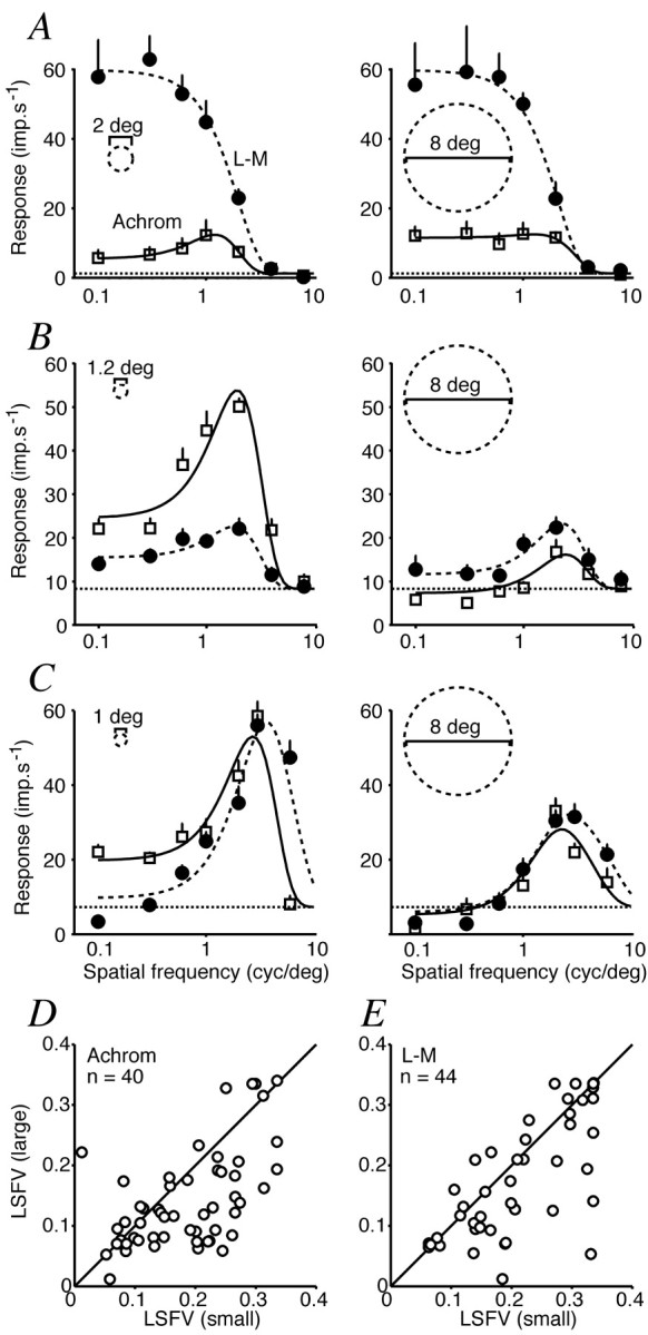
Effect of patch size on spatial frequency tuning of V1 cells. A-C, Each row shows for one cell the spatial frequency tuning curves for L-M gratings (filled circles) and achromatic ones (open squares) obtained with small (left column) and large (right column) patches. Smooth lines are best-fitting prediction of the difference-of-Gaussians model described in Results. Horizontal dashed lines show spontaneous activity. A, Simple cell that prefers L-M modulation. Responses at all spatial frequencies are little changed by changing patch size. B, Complex cell that shows low-pass spatial frequency tuning for L-M gratings in the small patch and bandpass in the large patch. The suppressive surround is most effective for achromatic gratings but also reduces low-frequency response for L-M. C, Complex cell that shows bandpass tuning for both achromatic and L-M gratings. The surround is effective at all spatial frequencies. D, Comparison of low-spatial frequency roll-off (LSFV; see Results for derivation) for cells that responded to achromatic gratings in both the small and large patch. Enlarging the patch increases the degree of low-spatial frequency roll-off. E, Similar plot for cells that responded to L-M gratings in both the small and large patch. Enlarging the patch increases the LSFV.
The remaining 39 neurons showed bandpass spatial frequency tuning for achromatic modulation in both small and large patches, although the depth of the low-frequency cut was generally greater with the large patches. When chromatic gratings were used, 14 of these neurons had low-pass tuning for L-M gratings when measured with a small patch (Fig. 13B). This kind of behavior would be expected from a neuron in which the spatially antagonistic subregions of the CRF had different spectral sensitivities (for example, different proportions of L- and M-cones in the excitatory and inhibitory regions, as in receptive fields of P-cells in lateral geniculate nucleus). Enlarging the patch had no effect on the spatial frequency tuning curves of six of the 14 cells, but for the remaining eight it caused the curve to become bandpass (Fig. 13B shows an example) or extinguished the response completely. Twenty-five other neurons showed bandpass spatial frequency tuning for L-M gratings in the small patch (Fig. 13C). This type of behavior often is used as an indicator of double-opponency: each spatial subregion in the CRF is itself cone opponent (Lennie et al., 1990; Johnson et al., 2001). In 22 of these neurons enlarging the patch revealed surround suppression and increased the loss of sensitivity at low spatial frequencies. Most neurons that showed bandpass spatial frequency tuning for large patches of L-M grating had surrounds sensitive to L-M modulation, particularly at low spatial frequency.
To summarize the effect of patch size on spatial frequency tuning, we calculated an index of low spatial frequency roll-off (LSFV) introduced by Xing and colleagues (Xing et al., 2002). This index combines information on both the slope and the magnitude of the LSFV and thus provides a more complete description of the tuning curve than either measure alone. The index can vary between 0 (in the extreme a cell responds to only one spatial frequency) and 0.35 (where a response to the lowest spatial frequency is at least as great as the response to any other frequency). The index is defined as:
 |
where Rf(i) is the amplitude of response at the ith spatial frequency (f) and fp is the peak spatial frequency. We obtained interpolated responses (Rf) by fitting a difference-of-Gaussians model (Enroth-Cugell and Robson, 1966) to the spatial frequency tuning curves (smooth lines in Fig. 13A-C) and then calculating the index in the range f(i) = fp/10... fp.
Figure 13D shows the index for large versus small patches of achromatic grating, and Figure 13E shows the comparison for L-M gratings. Only cells that responded above criterion to both patch sizes for the particular color direction are included. For both color directions increasing the patch size beyond the size of the CRF caused a reduction in the index, indicating that most cells showed greater LSFV in the larger patch. There are potential confounds in this measurement (even without a surround, a linear CRF will become slightly more bandpass as patch size is increased from a size smaller than it to one larger than it), but the effects shown in Figure 13 are much larger than can be explained by this and are consistent with a surround that prefers lower spatial frequencies than the CRF and augments the LSFV in whichever color direction to which it is sensitive.
Discussion
Construction of suppressive surrounds
The responses of most neurons in V1 and V2 were suppressed by extension of a grating patch beyond the classical receptive field, giving rise to size selectivity. The shapes of size-tuning curves often varied with the color direction used in measurement, in much the way they vary with achromatic contrast (Sceniak et al., 1999; Cavanaugh et al., 2002a). We used a model that assumes that CRF size is fixed but that the surround mechanism is less effective at low contrasts, thus revealing more of the CRF summation area (Cavanaugh et al., 2002a), and found that it characterized our measurements well when we allowed the CRF and surround to weigh differently the inputs from the three classes of cones.
The simplest account of our results is that in V1 the surround is relatively less sensitive to chromatic modulation than is the CRF. This is consistent with the idea that the signal of the surround is accumulated from a large pool of neurons with receptive fields in the region around the CRF (DeAngelis et al., 1994; Cavanaugh et al., 2002b; Müller et al., 2003). In V2, at least for those neurons that respond strongly to chromatic modulation, the surround has the same chromatic signature as the CRF and therefore exerts more powerful suppression when stimuli are modulated chromatically. This different behavior implies that the V2 surround arises within V2 and is not simply a reflection of what happens in V1.
Surround influence on chromatic tuning
One reason for undertaking the present study was to establish whether the chromatic tuning of the CRF depended on the chromaticity of light falling on the surround. Our results show clearly that it does not; although the effectiveness of surround suppression varies with the direction in which the surround is modulated in color space, for all directions of modulation the chromatic tuning of the CRF maintains a constant shape (Fig. 12). On this point our results agree with Zeki (1983a) and Moutoussis and Zeki (2002), who found in V1 and V2 that the preferred chromaticity of a receptive field was not altered by chromatic context. Our results do not agree with those of Wachtler et al. (2003), who found in V1 that the preferred chromaticity in the receptive field depended on the chromaticity of remote surrounding patches. Wachtler and colleagues worked with awake monkeys, and the remote influences they observed originated at distances from the receptive field (up to 5°) that would have elicited very little signal in the surrounds we studied. It therefore seems possible that in awake animals there is some additional contextual influence that arises in feedback from higher cortical areas.
Although the surround does not influence the chromatic tuning of the CRF, the surround can shape the overall chromatic tuning of the cell if its preferred chromaticity differs from that of the CRF. This is generally the case for simple and complex cells in V1; the preferred chromaticity of the CRF varies from cell to cell, whereas that of the surround tends to be constrained more narrowly around the achromatic axis. The upshot is that simple and complex cells are relatively more responsive to chromatic modulation when stimulated by large patches. The instability of chromatic preference is potentially troublesome for neurons that have a role in color vision. We wondered whether the underlying variation in chromatic tuning of the CRF might be unrelated to a role in color vision and instead simply might reflect the fact that the cell draws on all available L- and M-cones within the CRF so as to maximize its achromatic sensitivity. L- and M-cones are placed randomly in the photoreceptor mosaic (Roorda et al., 2001), so a CRF that draws inputs from all those available will have variable proportions of them in its subregions, giving rise to weak color opponency. Some of our results encourage this view: those neurons that responded to both chromatic and achromatic gratings had the smallest CRFs (Fig. 5) and therefore the greatest likelihood of unbalanced proportions of L- and M-cones in their subregions.
In both V1 and V2 the cells that responded most strongly to chromatic modulation in the CRF, and therefore the ones presumptively most relevant to color vision, had chromatic signatures that varied little with stimulus size. In V1 these had non-oriented receptive fields with low-pass spatial tuning (Lennie et al., 1990; Johnson et al., 2001). In an early study of such neurons Livingstone and Hubel (1984) explored receptive fields with spots of varying size and wavelength. They showed that the responsivity of some cells was reduced when a colored spot was made larger than optimal and inferred from this a “double-opponent” receptive field composed of concentric regions that received, for example, well balanced +L-M and +M-L cone inputs, respectively. Conway (2001) has described similar receptive fields. Such a receptive field would cause a neuron to respond much more robustly to chromatic than to achromatic gratings, with bandpass spatial frequency tuning for chromatic gratings. In V1 we saw no cells with receptive fields like this, although we did see many neurons that responded to both chromatic and achromatic gratings and showed bandpass spatial frequency tuning for both (Fig. 13) (Johnson et al., 2001). Most non-oriented cells in V1 that preferred isoluminant modulation showed no surround suppression at all; when such a cell did have a suppressive surround, it was usually weak and was insensitive to isoluminant stimuli. Ts'o and Gilbert (1988) have described “modified type II” cells that would have behaved like this. Most V2 neurons with CRFs that responded strongly to isoluminant modulation also had non-oriented receptive fields with low-pass spatial tuning but often had strong suppressive surrounds. Because the surround tended to be sensitive to the same isoluminant modulation as the CRF, the chromatic signature of a cell did not vary with stimulus size (Fig. 2F). Moutoussis and Zeki (2002) also found that the responses of color-preferring neurons in V2 were suppressed when a spot of optimal wavelength was made larger than the receptive field, although it is not clear whether this suppression was chromatically selective.
The size dependence of chromatic tuning in many neurons makes it important, in comparing findings from different studies, to know the size of the stimulus that has been used. This is especially the case for cells for which the CRFs respond to both chromatic and achromatic modulation. Lennie et al. (1990) used large patches of grating that covered both CRF and surround, thus maximizing the proportion of chromatically opponent cells. Johnson et al. (2001) used patches somewhat larger than the receptive field, but not large enough to cover the whole surround (Johnson et al., 2001), and would have identified relatively fewer chromatically opponent cells. The proportion of V1 cells identified here as opponent that uses small patches is similar to that found by Johnson et al. (2001), but the proportion identified as opponent that uses large patches is smaller than that found by Lennie et al. (1990). In this study we used gratings of low achromatic contrast and optimal spatial frequency to determine the chromatic signature of V1 neurons (Figs. 10, 11). Lennie et al. (1990) used gratings of higher achromatic contrast and often lower-than-optimal spatial frequency. We know (our unpublished data) that these differences would result in the present study yielding higher estimates of achromatic, but not chromatic, responsivity. This shift in the relative balance of achromatic and chromatic responsivity leads to us identifying relatively fewer cells as chromatically opponent.
Surround influence on spatial selectivity
We have shown (Fig. 13) that a V1 neuron for which the CRF has low-pass tuning can give rise to bandpass spatial frequency tuning when the surround also is stimulated. If the CRF already has bandpass tuning, that is often accentuated by surround stimulation. This is consistent with the surround preferring lower spatial frequencies than the CRF (DeAngelis et al., 1994; J. Müller and P. Lennie, unpublished observations). Our model of the surround conceives of it as having a Gaussian profile and hence being maximally sensitive under the CRF. This invites the question of whether the surround might be responsible for the low spatial frequency cut found with chromatically modulated gratings even when these are presented within a patch that does not extend beyond the CRF (Fig. 13C). Bandpass spatial tuning for chromatic gratings (Thorell et al., 1984; Lennie et al., 1990; Johnson et al., 2001) generally has been thought to require a receptive field with “double-opponent” organization. Most V1 cells that showed bandpass spatial frequency tuning to chromatic gratings within the CRF also had suppressive surrounds sensitive to chromatic gratings. Double-opponency, expressed as bandpass spatial frequency tuning to chromatic gratings, might arise simply because excitatory and inhibitory subregions of the CRF contain slightly different proportions of L- and M-cones, and the part of the surround lying under the CRF suppresses what otherwise would be strong responses at low spatial frequencies.
Relevance to perception
Psychophysical observations (Singer and D'Zmura, 1994; Clifford et al., 2003) show that the spatio-chromatic context in which a pattern is viewed can have a profound effect on its appearance. We think that the suppressive surrounds of V1 neurons are unlikely to be involved in these phenomena, because the surround is essentially absent from the receptive fields that are most obviously important for color vision and, even when present, does not influence the chromatic signature of the CRF. Transformations evident in V2 might be more relevant, because in V2 the surrounds can have substantial, chromatically selective effects on the sensitivity of the CRF of strongly opponent neurons.
Footnotes
This work was supported by National Institutes of Health Grants EY04440 and EY13079 and by Australian National Health and Medial Research Council Grant 211247 to S.G.S. We are grateful to J. A. Movshon and J. Krauskopf for helpful discussions, to J. Forte and C. Tailby for help during the experiments, and to R. Krane for histological reconstructions.
Correspondence should be addressed to Samuel Solomon, Center for Neural Science, New York University, New York, NY 10003. E-mail: samuels@cns.nyu.edu.
Copyright © 2004 Society for Neuroscience 0270-6474/04/240148-13$15.00/0
References
- Angelucci A, Levitt JB, Walton EJ, Hupe JM, Bullier J, Lund JS (2002) Circuits for local and global signal integration in primary visual cortex. J Neurosci 22: 8633-8646. [DOI] [PMC free article] [PubMed] [Google Scholar]
- Blakemore C, Tobin EA (1972) Lateral inhibition between orientation detectors in the cat's visual cortex. Exp Brain Res 15: 439-440. [DOI] [PubMed] [Google Scholar]
- Brainard DH (1996) Cone contrast and opponent modulation color spaces. In: Human color vision, 2nd Ed (Kaiser PK, Boynton RM, eds), pp 563-579. Washington, DC: Optical Society of America.
- Cavanaugh JR, Bair W, Movshon JA (2002a) Nature and interaction of signals from the receptive field center and surround in macaque V1 neurons. J Neurophysiol 88: 2530-2546. [DOI] [PubMed] [Google Scholar]
- Cavanaugh JR, Bair W, Movshon JA (2002b) Selectivity and spatial distribution of signals from the receptive field surround in macaque V1 neurons. J Neurophysiol 88: 2547-2556. [DOI] [PubMed] [Google Scholar]
- Clifford CW, Spehar B, Solomon SG, Martin PR, Zaidi Q (2003) Interactions between color and luminance in the perception of orientation. J Vis 3: 106-115. [DOI] [PubMed] [Google Scholar]
- Conway BR (2001) Spatial structure of cone inputs to color cells in alert macaque primary visual cortex (V1). J Neurosci 21: 2768-2783. [DOI] [PMC free article] [PubMed] [Google Scholar]
- DeAngelis GC, Robson JG, Ohzawa I, Freeman RD (1992) Organization of suppression in receptive fields of neurons in cat visual cortex. J Neurophysiol 68: 144-163. [DOI] [PubMed] [Google Scholar]
- DeAngelis GC, Freeman RD, Ohzawa I (1994) Length and width tuning of neurons in the cat's primary visual cortex. J Neurophysiol 71: 347-374. [DOI] [PubMed] [Google Scholar]
- Derrington AM, Krauskopf J, Lennie P (1984) Chromatic mechanisms in lateral geniculate nucleus of macaque. J Physiol (Lond) 357: 241-265. [DOI] [PMC free article] [PubMed] [Google Scholar]
- Desimone R, Schein SJ, Moran J, Ungerleider LG (1985) Contour, color and shape analysis beyond the striate cortex. Vision Res 25: 441-452. [DOI] [PubMed] [Google Scholar]
- De Valois RL, Cottaris NP, Elfar SD, Mahon LE, Wilson JA (2000) Some transformations of color information from lateral geniculate nucleus to striate cortex. Proc Natl Acad Sci USA 97: 4997-5002. [DOI] [PMC free article] [PubMed] [Google Scholar]
- Enroth-Cugell C, Robson JG (1966) The contrast sensitivity of retinal ganglion cells of the cat. J Physiol (Lond) 187: 517-552. [DOI] [PMC free article] [PubMed] [Google Scholar]
- Johnson EN (2001) Color signals in the macaque primary visual cortex. PhD thesis, New York University.
- Johnson EN, Hawken MJ, Shapley R (2001) The spatial transformation of color in the primary visual cortex of the macaque monkey. Nat Neurosci 4: 409-416. [DOI] [PubMed] [Google Scholar]
- Kiper DC, Fenstemaker SB, Gegenfurtner KR (1997) Chromatic properties of neurons in macaque area V2. Vis Neurosci 14: 1061-1072. [DOI] [PubMed] [Google Scholar]
- Lennie P, Krauskopf J, Sclar G (1990) Chromatic mechanisms in striate cortex of macaque. J Neurosci 10: 649-669. [DOI] [PMC free article] [PubMed] [Google Scholar]
- Levitt JB, Lund JS (1997) Contrast dependence of contextual effects in primate visual cortex. Nature 387: 73-76. [DOI] [PubMed] [Google Scholar]
- Levitt JB, Kiper DC, Movshon JA (1994) Receptive fields and functional architecture of macaque V2. J Neurophysiol 71: 2517-2542. [DOI] [PubMed] [Google Scholar]
- Livingstone MS, Hubel DH (1984) Anatomy and physiology of a color system in the primate visual cortex. J Neurosci 4: 309-356. [DOI] [PMC free article] [PubMed] [Google Scholar]
- Maffei L, Fiorentini A (1976) The unresponsive regions of visual cortical receptive fields. Vision Res 16: 1131-1139. [DOI] [PubMed] [Google Scholar]
- Mardia KV (1972) Statistics of directional data. In: Probability and mathematical statistics (Birnbaum ZW, Lukacs E, eds), pp 212-283. London: Academic.
- Monnier P, Shevell SK (2003) Large shifts in color appearance from patterned chromatic backgrounds. Nat Neurosci 6: 801-802. [DOI] [PubMed] [Google Scholar]
- Moutoussis K, Zeki S (2002) Responses of spectrally selective cells in macaque area V2 to wavelengths and colors. J Neurophysiol 87: 2104-2112. [DOI] [PubMed] [Google Scholar]
- Müller JR, Metha AB, Krauskopf J, Lennie P (2003) Local signals from beyond the receptive fields of striate cortical neurons. J Neurophysiol 90: 822-831. [DOI] [PubMed] [Google Scholar]
- Roorda A, Metha AB, Lennie P, Williams DR (2001) Packing arrangement of the three cone classes in primate retina. Vision Res 41: 1291-1306. [DOI] [PubMed] [Google Scholar]
- Sceniak MP, Ringach DL, Hawken MJ, Shapley R (1999) Contrast's effect on spatial summation by macaque V1 neurons. Nat Neurosci 2: 733-739. [DOI] [PubMed] [Google Scholar]
- Sceniak MP, Hawken MJ, Shapley R (2001) Visual spatial characterization of macaque V1 neurons. J Neurophysiol 85: 1873-1887. [DOI] [PubMed] [Google Scholar]
- Schein SJ, Desimone R (1990) Spectral properties of V4 neurons in the macaque. J Neurosci 10: 3369-3389. [DOI] [PMC free article] [PubMed] [Google Scholar]
- Shevell SK (1978) The dual role of chromatic backgrounds in color perception. Vision Res 18: 1649-1661. [DOI] [PubMed] [Google Scholar]
- Singer B, D'Zmura M (1994) Color contrast induction. Vision Res 34: 3111-3126. [DOI] [PubMed] [Google Scholar]
- Skottun BC, De Valois RS, Grosof DH, Movshon JA, Albrecht DG, Bonds AB (1991) Classifying simple and complex cells on the basis of response modulation. Vision Res 31: 1079-1086. [DOI] [PubMed] [Google Scholar]
- Thorell LG, De Valois RL, Albrecht DG (1984) Spatial mapping of monkey V1 cells with pure color and luminance stimuli. Vision Res 24: 751-769. [DOI] [PubMed] [Google Scholar]
- Ts'o DY, Gilbert CD (1988) The organization of chromatic and spatial interactions in the primate striate cortex. J Neurosci 8: 1712-1727. [DOI] [PMC free article] [PubMed] [Google Scholar]
- Wachtler T, Sejnowski TJ, Albright TD (2003) Representation of color stimuli in awake macaque primary visual cortex. Neuron 37: 681-691. [DOI] [PMC free article] [PubMed] [Google Scholar]
- Walraven J (1976) Discounting the background—the missing link in the explanation of chromatic induction. Vision Res 16: 289-295. [DOI] [PubMed] [Google Scholar]
- Wong-Riley M (1979) Changes in the visual system of monocularly sutured or enucleated cats demonstrable with cytochrome oxidase histochemistry. Brain Res 171: 11-28. [DOI] [PubMed] [Google Scholar]
- Xing D, Shapley R, Ringach DL, Hawken MJ (2002) Relationship between steady state orientation and spatial frequency tuning of macaque V1 neurons. Soc Neurosci Abstr 28: 456.7. [Google Scholar]
- Zeki SM (1983a) Colour coding in the cerebral cortex: the reaction of cells in monkey visual cortex to wavelengths and colours. Neuroscience 9: 741-765. [DOI] [PubMed] [Google Scholar]
- Zeki SM (1983b) Colour coding in the cerebral cortex: the responses of wavelength-selective and colour-coded cells in monkey visual cortex to changes in wavelength composition. Neuroscience 9: 767-781. [DOI] [PubMed] [Google Scholar]