Adaptive Temporal Integration of Motion in Direction-Selective Neurons in Macaque Visual Cortex

Abstract

Direction-selective neurons in the primary visual cortex (V1) and the extrastriate motion area MT/V5 constitute a critical channel that links early cortical mechanisms of spatiotemporal integration to downstream signals that underlie motion perception. We studied how temporal integration in direction-selective cells depends on speed, spatial frequency (SF), and contrast using randomly moving sinusoidal gratings and spike-triggered average (STA) analysis. The window of temporal integration revealed by the STAs varied substantially with stimulus parameters, extending farther back in time for slow motion, high SF, and low contrast. At low speeds and high SF, STA peaks were larger, indicating that a single spike often conveyed more information about the stimulus under conditions in which the mean firing rate was very low. The observed trends were similar in V1 and MT and offer a physiological correlate for a large body of psychophysical data on temporal integration. We applied the same visual stimuli to a model of motion detection based on oriented linear filters (a motion energy model) that incorporated an integrate-and-fire mechanism and found that it did not account for the neuronal data. Our results show that cortical motion processing in V1 and in MT is highly nonlinear and stimulus dependent. They cast considerable doubt on the ability of simple oriented filter models to account for the output of direction-selective neurons in a general manner. Finally, they suggest that spike rate tuning functions may miss important aspects of the neural coding of motion for stimulus conditions that evoke low firing rates.

Introduction

Motivated by the idea that the visual cortex is a spatial frequency (SF) and temporal frequency (TF) analyzer, the responses of direction-selective (DS) neurons are commonly modeled using linear filters that are oriented in space-time (Fahle and Poggio, 1981; Watson and Ahumada, 1983; van Santen and Sperling, 1984; Adelson and Bergen, 1985). These models have gained wide use in physiologically inspired computer simulations of motion perception (Heeger, 1987; Grzywacz and Yuille, 1990; Nowlan and Sejnowski, 1995; Simoncelli and Heeger, 1998) and have received additional support from experimental studies (Reid et al., 1991; Emerson et al., 1992; Emerson, 1997; De Valois et al., 2000; Touryan et al., 2002). If the response of a DS neuron can be described effectively by such simple combinations of spatiotemporal filters, then the envelop of the filter, essentially the receptive field (RF) profile, should be stable for a given cell and easily mapped in space and time (Touryan et al., 2002).

However, psychophysical studies show that the temporal profile of motion integration is not stable but varies with stimulus speed, SF, and contrast (Nachmias, 1967; Vassilev and Mitov, 1976; Breitmeyer and Ganz, 1977; Thompson, 1982; Van Doorn and Koenderink, 1982; De Bruyn and Orban, 1988; Müller and Greenlee, 1998; Burr and Corsale, 2001; Vassilev et al., 2002). Could these stimulus-related changes at the perceptual level originate from changes in the properties of single cortical DS cells, or do they simply reflect a population of diverse, but individually fixed, temporal RF profiles? Fixed RFs are consistent with demonstrations that linear spatiotemporal filters account well for response properties including direction selectivity in V1 simple cells (Movshon et al., 1978; Reid et al., 1987; McLean and Palmer, 1989, 1994; DeAngelis et al., 1993), but there have been some reports of stimulus-related changes in temporal integration in simple and complex cells in cats and monkeys (Dean et al., 1982; Reid et al., 1992).

To determine whether the temporal RFs of DS cells are fixed, we presented randomly moving stimuli, essentially coarse approximations to white noise in the velocity domain (de Ruyter van Steveninck and Bialek, 1988; Bair et al., 1997; Buračas et al., 1998; Borghuis et al., 2003), and computed spike-triggered averages (STAs) (de Boer and Kuyper, 1968) to estimate first-order profiles of temporal integration across multiple stimulus conditions. We tested complex DS cells in V1 because V1 is where direction selectivity originates (Hubel and Wiesel, 1962) and these cells have been closely compared with sets of motion filters. We also tested DS cells in MT/V5 (Zeki, 1974), which have much larger RFs (Gattass and Gross, 1981; Albright and Desimone, 1987) and can be selective for global pattern motion (Movshon et al., 1985). This allowed us to compare responses in V1 with those at a higher level in which DS responses have been closely linked to motion perception (for review, see Parker and Newsome, 1998). We did not examine DS simple cells because the spatial phase dependence of their responses calls for a more elaborate stimulus paradigm and makes them less directly comparable with MT cells. In both V1 and MT, we found that the temporal profiles reflected by the STAs changed substantially with the spatiotemporal structure and contrast of the stimuli. We also presented our visual stimuli to a model DS unit consisting of a set of motion energy (ME) filters (Adelson and Bergen, 1985) and an integrate-and-fire (IF) spiking mechanism. The model did not capture the changes in the STAs observed in the vast majority of our DS neurons. Our results strongly suggest that DS responses in V1 and MT cannot be accounted for by standard models with fixed profiles of temporal integration. Rather, the responses reflect a system that changes its integration properties with stimulus parameters in a manner consistent with psychophysical observations.

Materials and Methods

Electrophysiology

We recorded extracellularly from the primary visual cortex of anesthetized, paralyzed macaque monkeys (two Macaca nemestrina and eight Macaca fascicularis). Detailed methods for this type of recording were described by Cavanaugh et al. (2002). Experiments typically lasted from 4 to 5 d, during which anesthesia and paralysis were maintained with sufentanil citrate (4-6 μg/kg/hr) and vecuronium bromide (Norcuron; 0.1 mg/kg/hr), respectively, administered in lactated Ringer's solution (8 ml/kg/hr) containing dextrose (2.5%). Artificial respiration with moist room air was maintained with rate adjustments to keep expired CO₂ between 3.8 and 4.0%. Body temperature was maintained near 37°C with a heating pad. EEGs and electrocardiograms were monitored to ensure proper depth of anesthesia. All procedures conformed to guidelines of the New York University Animal Welfare Committee.

Tungsten-in-glass microelectrodes (Merrill and Ainsworth, 1972) were advanced with a hydraulic microdrive downward through a craniotomy of 9-10 mm diameter. In some experiments, we used a mechanical microdrive system with quartz-platinum/tungsten microelectrodes (Thomas Recordings, Marburg, Germany). For V1, the craniotomy was typically centered 4 mm posterior to the lunate sulcus and 10 mm lateral to the midline. Neurons in V1 were recorded both on the operculum and in the calcarine sulcus (typical RF eccentricities were 1-6° and 8-20°, respectively). For MT, the craniotomy was centered 15 mm lateral to the midline, 4 mm posterior to the lunate sulcus, and the angle of advance was 20° down (relative to horizontal) and forward in the parasaggital plane. Action potentials were detected using a hardware dual-window time-amplitude discriminator (Bak, Mount Airy, MD) and time stamped at a resolution of 0.25 msec. Electrolytic lesions (2 μA for 2-5 sec) were made for histological verification and estimation of cortical layer. At the end of experiments, animals were given an overdose of sodium pentobarbitol (30-60 mg/kg), exsanguinated through the heart, and perfused with 4% paraformaldehyde in saline.

Visual stimuli

Visual stimuli were generated by custom software on a CRS 2/2 Board (Cambridge Research Systems, Kent, UK) and presented on a standard cathode ray tube (CRT) at 100 Hz vertical refresh with a mean luminance 33 cd/m². The CRT was placed farther from the monkey's eye for smaller neuronal RFs and closer for larger RFs. The distance ranged from 80 to 180 cm, for which the screen covered ∼10-20° of visual angle. Stimuli were presented on a mean gray background and, except where noted, at 100% Michelson contrast (100% nominal contrast is ∼98% actual contrast because the minimum luminance on our CRT was ∼0.5 cd/m²).

Basic characterization with drifting sine waves. We mapped the RF for each cell by hand with patches of drifting sinusoidal gratings to estimate values of four parameters (orientation, SF, TF, and patch size) of the grating that maximized the firing rate of the cell. We then used a small patch of optimal grating to determine the RF center. After hand mapping, we ran four computer-controlled experiments to systematically and sequentially optimize the four stimulus parameters in the order listed above. In each experiment, trials were interleaved in a blockwise random manner, and grating stimuli were presented in a circular aperture for 2-4 sec with 2 sec of mean gray between trials. Direction of motion, which was always perpendicular to orientation, was tested at 22.5° increments. We will refer to the direction eliciting the largest response as the preferred direction and that 180° opposite as antipreferred. SF was tested at half-octave steps over a five-octave range that was approximately centered on the optimal SF. TF was tested in octave increments from 0.2 to 25 Hz. Finally, the diameter of the grating patch was tested over a five-octave range. We defined the classical RF size to be the smallest diameter that produced at least 95% of the maximum response (for details, see Cavanaugh et al., 2002).

We classified cells in V1 as simple or complex on the basis of their modulation index, MI = F1/DC, in response to an optimal drifting grating (Skottun et al., 1991). Here, DC is the mean evoked firing rate (in excess of the spontaneous firing rate to a mean gray field), and F1 is the amplitude of the Fourier component of the response at the stimulus TF. We will refer to V1 cells with MI ≤ 1 as complex. For all cells, we computed a direction index, DI = 1 - a/p, where p and a are the evoked firing rates for the preferred and antipreferred directions of motion (Maunsell and Van Essen, 1983). If a cell fired equally for both directions, then DI = 0. Cells that were strongly direction selective had a DI near 1. Values of DI > 1 indicate that the antipreferred stimulus suppressed the firing rate below the spontaneous rate. All cells studied here had DI > 0.7 (two of the V1 cells had DI < 0.8) and will be referred to as direction selective.

Random motion stimuli. After the initial characterization, we tested each DS cell with dynamic stimuli in which an optimally oriented sinusoidal grating moved randomly back and forth along the axis of preferred motion of the cell. Specifically, the spatial phase of the grating was shifted between successive video frames (every 10 msec) by either +Δ or -Δ, where Δ was fixed and ≤1/4 spatial cycle of the grating. A shift of +Δ generated motion in the preferred direction, whereas a shift of -Δ generated an antipreferred motion. Figure 1 A shows a sequence of four stimulus frames (numbered 1-4) in which the grating moves in the antipreferred direction (downward) by 1/4 cycle between the first and second frames (downward arrow) and then moves in the preferred direction (upward) on the next two frames (upward arrows). The stimulus performed a binary random walk along the axis of preferred motion, and the movements were governed by a pseudorandom sequence generated either from the ran2 algorithm of Press et al. (1992) or from a binary m-sequence (Sutter, 1987; Reid et al., 1997).

Figure 1.

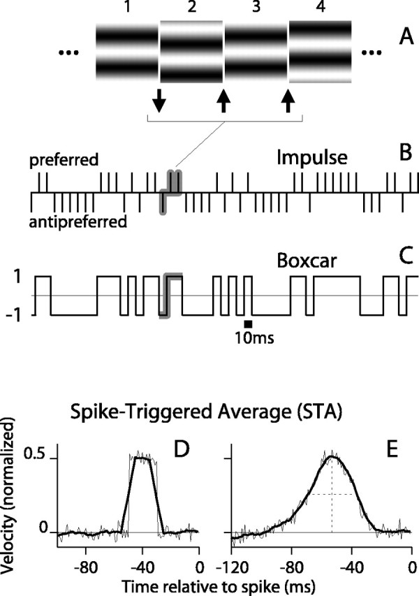
The random motion stimulus and the computation of the STA. A, A sequence of four frames of the visual stimulus in which the optimal grating is shifted by 90° of phase in either the preferred (upward; up arrows) or antipreferred (downward; down arrow) direction between frames. B, The impulse representation of a 500 msec segment of stimulus is shown. The amplitude and sign of the impulses represent the size and direction of the motion (the displacement of the grating) between frames. C, The boxcar representation of the same stimulus segment takes the value 1 or -1 if the most recent movement was preferred or antipreferred, respectively. It can be constructed by convolving the function in B with a 10 msec wide boxcar. D, STAs were computed for spike trains from a model with a square window of temporal integration of duration 20 msec. The STA (thick line) computed from the boxcar stimulus was smoother than that (thin line) computed from the impulse stimulus. E, STAs computed for neuronal data. The STA (thick line) computed from the boxcar stimulus is smoother and virtually no different in shape than that (thin line) computed from the impulse stimulus.

Rather than quantify the speed of the random motion in terms of Δ (the phase shift per video frame), we define a more convenient value called equivalent temporal frequency (ETF), which is the change in phase, Δ, divided by the change in time, 10 msec. The ETF is the TF of a grating that drifts in one direction with a phase shift of Δ on each video frame. Our fastest random motion stimulus had ETF = 25 Hz (1/4 cycle per 10 msec).

The advantage of using the random motion stimulus is that temporal integration can be mapped with stimuli having a variety of spatial and temporal structure, allowing us to determine how the operation of the visual system changes when it is confronted with different visual contexts. We will examine results from experiments in which one of three parameters varied: the ETF of the motion, the SF of the grating, or the contrast of the grating. In each experiment, the random motion stimuli were presented in trials of duration 20-40 sec and separated by 2 sec of mean gray. Motion on each trial was governed by a different random sequence.

Data analysis

Representation of stimulus and response. We represented the spike trains and the visual stimuli as discrete functions of time at a 1 msec resolution. The spike trains were 1 when a spike occurred and 0 everywhere else. We defined two representations of the random motion stimulus. The impulse representation uses positive and negative impulses to represent the displacements of the grating between frames (Fig. 1 B). The boxcar representation is generated by convolving the impulse representation with a 10 msec wide boxcar function, effectively replacing each impulse by a 10 msec boxcar centered on the impulse (Fig. 1C). The boxcar representation has only two values, a positive value for preferred motion and a negative value for antipreferred motion. When these values are defined to be 1 and -1, the stimulus is normalized (it has mean of 0 and variance of 1) and it may be thought of as a normalized velocity signal.

Computation of the STA. We used the method of spike-triggered averaging (De Boer and Kuyper, 1968) to quantify the relationship between the spike train and the motion in the random stimulus. The STA was computed by averaging together fixed-length segments of the stimulus that preceded each spike. Each stimulus segment was aligned to the time of the spike, defined as t = 0. This is equivalent to computing the cross-correlation function for the spike train and the stimulus and examining only the half for which the stimulus precedes the spikes. With the normalized boxcar representation of the stimulus, the STA ranged from -1 to 1.

We used the STA to estimate the temporal profile of motion integration; therefore, it is important to consider how the choice of stimulus representation impacts the shape of the STA. Using the boxcar stimulus essentially convolves the STA with a boxcar function. For example, consider a system that sums the motion stimulus within a rectangular window of width 20 msec and fires spikes at random at a rate proportional to this sum. This system has a known window of integration: a 20 msec wide rectangle. The STA computed with the impulse stimulus accurately reflects the rectangular structure of the integration window (Fig. 1 D, thin line), whereas the STA computed from the boxcar stimulus (thick line) has sloped ends, reflecting the boxcar convolution. However, the latter STA is smoother and its basic features (e.g., its height and width) are very similar to those of the STA computed from the impulse stimulus. When a more realistic, rounded window is used, there is almost no difference in shape between the STAs computed with the impulse and boxcar stimulus representations. This is demonstrated in Figure 1 E for neuronal data. The STA computed with the boxcar stimulus (thick line) is a smoother version of the STA computed with the impulse stimulus (thin line).

In summary, we will use the boxcar representation to compute STAs because of the smoothing that it offers, but with the understanding that it cannot resolve features at a temporal resolution below 10 msec. Furthermore, this representation allows us to interpret the vertical axis of the STA as a scaled probability. In particular, the probability that the movement that occurred closest to time t was preferred is 1 if STA(t) = 1 and 0.5 if STA(t) = 0. It is worth noting that the STA does not by itself provide information about the firing rate; it simply reveals the probability that the stimulus moved in the preferred direction at various times before a spike.

To quantify the shape of STA peaks, we computed the height and the width at half-height for each peak that met a statistical criterion. We called a peak in the STA significant if the average value across any 40 msec window within the epoch from -200 to 0 msec was at least five times the SD computed for the 20 nonoverlapping 40 msec windows in the period from -1000 to -200 msec. This criterion not only ensured that we analyzed STA peaks that were statistically significant, but also that the peaks were substantial enough to provide accurate measurements of peak height and width. We found that broad STA peaks were, in general, noisier because by necessity they either had low amplitudes or arose at lower firing rates. Therefore, we convolved such STAs with a Gaussian (SD, 4 msec) if their width at half-height, determined after smoothing, was >40 msec. This removed high-frequency noise that was not removed by the boxcar smoothing because of the sharp edges of the boxcar function.

We examined STAs in the frequency domain by computing the Fourier transform (FT) of the STA. We used STAs that were 512 msec long, centered at t = -80 msec, and multiplied them by a Gaussian window (mean, -80; SD, 80 msec) to suppress noise at the tails. The high-frequency cutoff was defined to be the point at which the amplitude of the FT of the STA fell to half of its maximum value. If the amplitude at low frequencies also fell to less than half of the maximum, the STA was classified as bandpass.

Information theoretic calculation. We used a modification of the direct information theoretic technique of Liu et al. (2001) to compute how much entropy was shared by the random motion stimulus and the response. Given a particular stimulus sequence, we used the STA to estimate the probability of a spike at a given time rather than computing that probability directly from the raw spike trains. Specifically, we estimated the mutual information between a segment of the stimulus and the predicted neuronal response in a 1 msec bin at time t_o relative to the beginning of the stimulus segment. The stimulus segment was made long enough to include the region of the STA that differed substantially from zero, its length being T = mΔt, where m is the number of stimulus movements (typically 16) and Δt = 10 msec. The mutual information (Cover and Thomas, 1991) between the stimulus X and the response Y is as follows:

1

2

where is the binary entropy function [], p_i is the probability of a spike at t_o given stimulus s_i (i = 1,..,n = 2^m), and p̄ is the mean of p_i over all i. The spike probability for s_i is computed from the response, r_i, to the stimulus:

3

where STA(t) is the STA. The probability of a spike is determined by:

4

where... + is half-wave rectification, r_thresh is the rectification threshold, and α is set to match the mean firing rate of the response from which the STA was computed. We estimated r_thresh, which is a non-decreasing function of STA amplitude, using an iterative, binary search until a value was found for which the resulting STA amplitude for the model (Eq. 4) was within 1% of that observed for the neuronal STA. We applied the method described in Equations 1-4 to compute I(X;Y) for increasing t_o until an asymptote was reached [asymptoting behavior is described by Liu et al. (2001), their Fig. 15]. We averaged the value of I(X;Y) in a 10 msec period after the asymptote was reached (typically 160-170 msec after the start of the stimulus segment). This value, in units of bits, was converted into a rate by dividing by the 1 msec bin size, and this was then divided by the spike rate to produced a value with units of “bits/spike” (Liu et al., 2001). Care is required when interpreting this value. It does not capture any information that might be present in the temporal relationships between spikes because we have estimated only the information between the stimulus and the occurrence (or not) of a spike in a single time bin. However, at low spike rates (sometimes <1 spike/sec), there is no practical way to estimate such relationships. We will use this value only for comparing stimulus conditions to each other based on the shape of the STAs.

We computed the STA implied by Equation 4 and verified that it matched the STA from the neuronal responses. For several cells and stimulus conditions with very high firing rates, we were able to compare the results of our STA-based method to results computed directly from the spike trains using the method of Liu et al. (2001). We found these results matched very closely for short stimulus segments (six to eight letters, or 60-80 msec), which were the only ones for which the spike-train method had a negligible bias.

Simulation of a spiking motion detector

We compared the neuronal STAs with those produced by a common model for cortical direction selectivity, the ME model (Adelson and Bergen, 1985). The first stage of the model was a pair of oriented, linear space-time filters constructed as the product of Gaussians and sinusoids (Grzywacz and Yuille, 1990):

5

where r = (x,y) is the spatial position vector, t is time, f_r is the SF, f_t is the TF, σ_r is the SD of the spatial Gaussian, σ_t is the SD of the temporal Gaussian, and n = (cosθ, sinθ) is the normal vector defining the spatial orientation and direction of the sinusoid in terms of the angle θ. The real and imaginary parts of Equation 5 represent the two quadrature filters of the complex DS cell model. We will use G⁺ to refer to the quadrature filter pair for the preferred direction of motion and G- to refer to the filter pair for antipreferred motion, which is derived by replacing n with -n.

The square of the modulus of the convolution of the input image intensity, I(r,t), with the filters yields the local motion energies in the preferred and antipreferred directions in space and time:

6

7

The responses in time for the preferred and antipreferred motion detectors located at the center of the image, r = (0,0), are, respectively, as follows:

8

9

The motion model was simulated on a discrete grid (32 × 32 pixels) with a spatial resolution of 0.2°/pixel and a temporal resolution of 2 msec. The temporal dimension was matched to the duration of the stimulus being tested. The parameters of the motion filters were set to match a typical V1 complex DS neuron as follows: σ_r = 0.18°, σ_t = 15 msec, f_r = 1.25 cycles/degree, f_t = 10 Hz, θ = 0. The input image sequence, I(r,t), had luminance values ranging from 0 to 1, corresponding to the maximum and minimum luminance in our stimuli, and was modulated in space and time to mimic the visual stimuli presented to the neurons.

Outputs of the ME computation served as inputs to an IF neuronal model. The intracellular voltage, V, of the model neuron obeyed the equation:

10

where C is the membrane capacitance, V_ex and V_in are reversal potentials for the excitatory and inhibitory conductances, g_ex and g_in, respectively, and V_rest is the reversal potential for the leak conductance, g_leak. When V reached V_thresh, a spike was discharged and V was set to V_reset. To implement a refractory period, V was held at V_reset for 1.5 msec after each spike. The excitatory and inhibitory conductances were proportional to p(t) and a(t) (Eq. 9) with added noise as follows:

11

12

where n_p(t) and n_a(t) were Gaussian filtered (SD, 1 msec), Gaussian white noise (mean, 20 nS; SD, 5 nS), and c_ex = 0.35 nS and c_in = 1.0 nS [the ME outputs p(t) and a(t) are unitless]. Values of the other parameters were C = 500 pF, V_ex = 0, V_in= -70 mV, g_leak = 75.0 nS, V_leak= -73.6 mV, V_thresh = -52.5 mV, and V_reset = -56.5 mV (values of Troyer et al., 1998). The voltage equation was simulated using a fifth-order Cash-Karp Runge-Kutta method with adaptive step size (Press et al., 1992).

We chose to use an opponent model in which inhibition from an antipreferred motion opposes the excitation from preferred motion because of observations that an antipreferred motion has a suppressive influence on the neuronal response. In particular, an antipreferred motion often suppresses spontaneous firing, and it delays the subsequent responses to preferred motion (Bair et al., 2002). We performed some simulations on the IF model in isolation by explicitly manipulating g_ex(t) while holding g_in(t) = 0. We generated g_ex(t) as a binary random sequence like that shown in Figure 1C for a particular mean and SD. Negative conductance values, if they occurred, were set to zero. STAs were computed from 6 min of simulated time.

Results

We examined the temporal integration of motion in 48 complex DS cells in V1 and 40 DS cells in MT. For each population, Table 1 summarizes some commonly reported response measures and RF properties derived from our standard characterization of each cell. After determining the preferences of each cell for drifting sinusoidal gratings, we assessed the temporal profile of the RF using our random motion stimulus, and we quantified how temporal integration changed with three stimulus parameters: speed, SF, and contrast. Not all parameters were varied for each cell (numbers are given below). After describing the neuronal data, we applied the same techniques to characterize a widely used model of motion detection and a simple mechanism of spike generation.

Table 1.

Basic characterization of V1 complex DS and MT cells

	V1 (n = 48)	MT (n = 40)
Spontaneous rate (spikes/sec)	4.9 ± 7.1	8.2 ± 6.1
Maximum rate (spikes/sec)	87 ± 46	57 ± 19
Modulation index	0.21 ± 0.15	0.21 ± 0.10
Direction index	0.99 ± 0.09	1.09 ± 0.14
Direction bandwidth (degrees)	70 ± 26	98 ± 39
RF eccentricity (degrees)	7 ± 6	15 ± 12
CRF diameter (degrees)	1.8 ± 1.7	8.0 ± 4.2
Optimal SF (cycles/degree)	1.9 ± 1.1	0.9 ± 0.6
Optimal TF (Hz)	7.8 ± 5.5	11.5 ± 7.9

Values are mean ± SD. Spontaneous rate is the response to a mean gray field. Maximum rate is the average response during the first 2 sec of the optimal drifting grating. See Materials and Methods for modulation and direction indices. Direction bandwidth is the width at half-height of the peak in the direction tuning curve. RF eccentricity is the visual angle between the fixation point and the center of the RF, which ranged from 1.0 to 21° in V1 and from 2.2 to 35° in MT. Optimal SF and TF are those that produced the maximum firing rate for drifting gratings. CRF, Classical receptive field.

Stimulus speed and neuronal integration time

To test the dependence of integration time on speed, we presented our random motion stimulus at various step sizes, Δ, ranging from 1/1024 to 1/4 cycle, in octave steps, while holding the SF of the grating at the optimal value for the cell. The phase shifts for this range of Δ correspond to temporal frequencies from 0.1 to 25 Hz, which we will refer to as equivalent TFs, or ETFs. The speed of a moving grating equals TF/SF, so for a typical SF of 1 cycle/degree (Table 1), the range of speeds tested was 0.1-25°/sec. For human observers, scrutiny was required to detect motion in the slowest of the nine stimuli, whereas the fastest stimulus appeared blurry and of lower contrast because of its rapid motion.

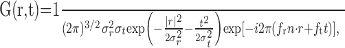
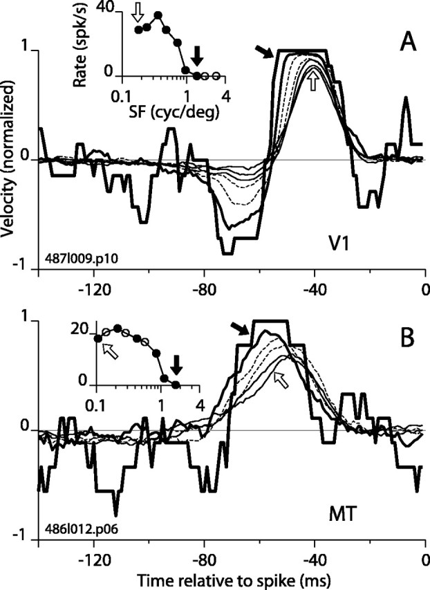
We recorded responses from 31 V1 complex DS cells and 21 MT cells for these stimuli and assessed the profile of temporal integration by calculating the STA, which is the average of all stimulus segments that preceded a spike. For an example V1 cell, the STAs for a subset of the ETFs are shown in Figure 2A. The STA for the fastest motion (ETF, 25 Hz) had the tallest and narrowest peak (thin solid line), and as the ETF was decreased, the STA height decreased. The inset in Figure 2A plots the mean firing rate for each ETF. The filled circles in the inset correspond to the six STAs shown in the main panel (arrows mark correspondence for two cases). Two important facts are immediately obvious. First, the STA peaks are not scaled versions of each other; the peaks are wider and extend further back in time for slower motion. Second, the variation in the shape of the STA is not simply related to the change in mean firing rate. For example, the firing rates for ETFs of 1.6 and 25 Hz were the same, yet the STAs differed markedly (Fig. 2A, open and filled arrows). A set of STAs for an MT cell is shown in Figure 2B. Progressing from the fastest to the slowest stimulus, the firing rate decreased steadily (Fig. 2B, inset), but the STA width increased only after the ETF dropped below <1 Hz (e.g., STA at open arrow). The STA peak heights for this cell varied little with stimulus speed when compared with the example in Figure 2A. Thus, the STA peak for slow motion was both wide and tall (Fig. 2B, thickest solid line). Such a peak indicates that the discharge of a spike typically required the occurrence of several consecutive preferred movements. These two examples represent a range of behavior that was observed in both V1 and MT, and they do not represent systematic differences between these two areas.

Figure 2.

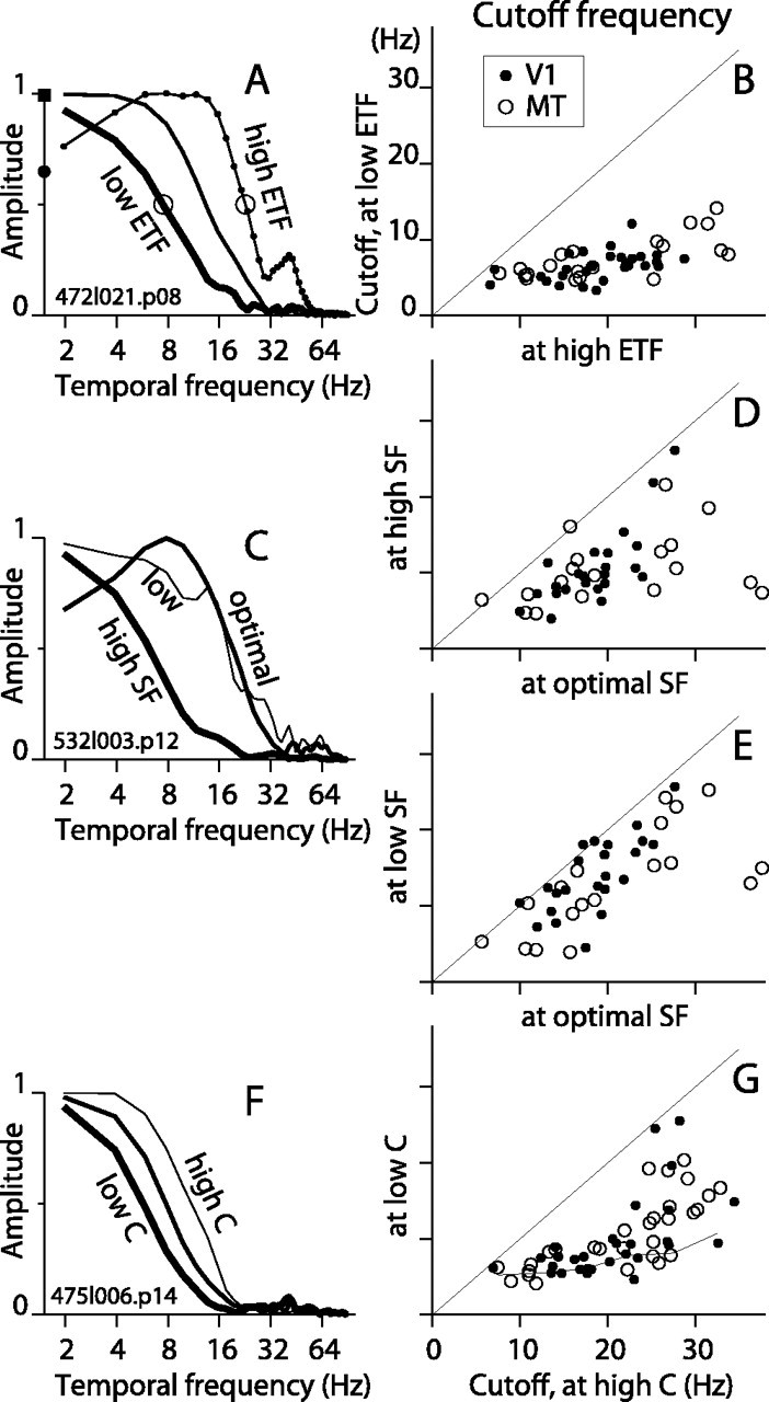
STAs as a function of stimulus ETF. A, STAs for six ETFs are plotted for an example V1 complex DS cell. In the inset, the mean firing rate is plotted for all nine ETF values tested, and the dashed line shows the spontaneous rate. In the main panel, STAs are shown only for the solid points in the inset. The arrows mark corresponding points and STA curves. The line style legend (square box) shows the progression from low to high ETF. B, STAs formatted as in A are shown for an example MT cell. Here and in A, STAs are wider for slower motion (i.e., lower ETF). C, The average width at half-height of the STA peak is plotted against ETF for 31 V1 cells and 21 MT cells. The error bars show SEM. D, The average height of the STA peak is plotted against ETF. E, The average of the product, height × width, is plotted against ETF. F, The asymptotic value of the mutual information between the stimulus and the response (calculated from the STA) in a 1 msec bin was divided by the bin width, and this measure was then divided by spike rate (see Materials and Methods). G, The mean firing rate in excess of the spontaneous rate is plotted against ETF.

The patterns observed in the examples suggest that the temporal integration of motion reflected by the width of the STAs was not constant but varied with stimulus speed. Specifically, for rapidly moving stimuli, the spike of a DS cell signaled the occurrence of preferred motion in a relatively recent and brief time window. For slow motion, however, a spike from the same neuron signaled preferred motion over a longer time window that extended farther into the past. In other words, the broadening of the STA peak resulted from a substantial leftward shift of the left side of the peak, whereas the right side shifted much less (as seen in Fig. 2B) and often appeared to simply lean more to the left (Fig. 2A). This behavior occurred in all of the cells that we studied. A less consistent feature of STAs was a negative lobe to the left of the positive peak (Fig. 2A, thinnest line). This dip indicates that motion in the antipreferred direction facilitated the response to subsequent preferred motion. The dip is associated with transient responses to preferred motion and can arise from various mechanisms, including spike rate adaptation and synaptic depression, both of which can make responses more transient. In an extreme case in which a cell fires only transiently at the onset of preferred motion, the dip and the positive peak can have equal area (data not shown). However, the dips were almost always small compared with the positive peak, so we will focus on the latter.

To quantify the most prominent changes in the STA peaks across our database, we computed the height and the width (at half-height) for each STA peak that was >5 SDs above the noise (see Materials and Methods). Figure 2C shows that the mean peak width changed as a function of ETF for V1 and MT, increasing from ∼20 msec for fast motion to 50-70 msec for slow motion. The data for V1 and MT followed a common trend for ETFs of 1 Hz, but for slower stimuli, the STAs for MT were broader than those for V1. The difference between V1 and MT at slow speeds may be greater than it appears, because more V1 than MT cells failed to meet our STA peak criterion at low ETF. For example, at the second lowest ETF, 20 of 21 STAs met the criterion for MT, whereas only 16 of 31 did for V1. At the lowest ETF, this dropped to 13 of 21 for MT and 12 of 31 for V1. The average height of the STA peaks is plotted in Figure 2D. Peaks were tallest, on average, at an ETF of 12.5 Hz (Fig. 2D) and decreased by approximately half at the lowest speeds for both V1 and MT. To verify that curves in Figure 2, C and D, were not affected by having fewer cells at the lowest ETFs, we recomputed the curves using data from only those cells that had significant STA peaks at all ETFs. These curves were very similar to those shown.

Taller STA peaks indicate that, given the occurrence of a spike, the direction of motion is known with greater probability, and wider peaks indicate that the direction can be estimated over a longer epoch. Therefore, to get an approximate estimate of how informative a single spike was about the recent stimulus motion, we multiplied the peak width and height to approximate the area of the STA peak. Figure 2E shows that the area was largest at rather low ETFs, from 0.5 to 1 Hz. At the lowest ETFs, the area decreased sharply in V1 (Fig. 2E, thick line) because the STA peaks collapsed without increasing in width. In MT, however, the average peak area (for the 62% of cells that still met the 5 SD criterion) remained near its maximum value at the lowest ETF. These results imply that under conditions of very slow change in the visual image the occurrence of a single spike can convey a substantial amount of information. To make a more rigorous estimate of the information conveyed by a single spike, we used the entire STA (from t = -180 to -20 msec), not just the positive peak, as a basis for computing the mutual information between a spike and the pattern of movements in the stimulus (see Materials and Methods). These mutual information values were strongly correlated to the STA area values (r = 0.85 for V1; r = 0.62 for MT; p < 0.0001 for both). The mean mutual information, expressed in bits per spike, is plotted in Figure 2F as a function of ETF. Because the information metric favors height over width in the STA peak, the maximum values on these curves lie at higher ETFs (for which STA peaks are taller) compared with the maximum values on the area curves. Nevertheless, the trend in both sets of curves differed strikingly from that for the mean firing rate (Fig. 2G), which peaked near the highest ETFs and dropped off sharply at medium to low ETFs. Thus, a single spike often conveyed as much or more information about the motion of the stimulus under conditions in which the stimulus was substantially suboptimal for the cell in terms of firing rate.

In summary, for all DS cells that we studied, the STA peak grew wider by spreading back in time for slower moving random stimuli. This indicates that the effective integration time of the computations underlying DS responses in cortex changes with stimulus conditions. The integration time for the slowest motion that we tested was, on average, approximately two to four times longer than that for the fastest motion.

Spatial frequency and integration time

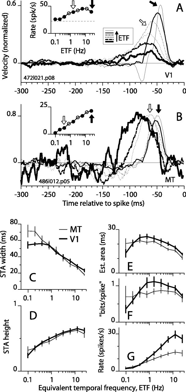
We tested whether the temporal integration of motion also depended on SF by presenting the random motion stimulus at a variety of SFs, including values well below and well above the optimal SF of each cell (determined for smoothly drifting gratings). We held the step size, Δ, constant at 1/8 of the spatial period. Thus, the ETF remained constant at 12.5 Hz, which was optimal or near optimal in terms of the height of the STA peak (Fig. 2D) and evoked firing rate (Fig. 2G) for most cells.

Figure 3A shows how the STA shape changed with changes in SF for an example V1 complex DS cell that had an optimal SF of 3 cycles/degree. For clarity, STAs are plotted for only six of the nine SFs tested (Fig. 3A, line style legend below panel shows progression from low to high SF). Progressing from the lowest to the optimal SF, the STA peak remained narrow and the peak height increased somewhat (Fig. 3A, progression from thin solid line to the line of shortest dashes). For SFs above the optimal, the STA peak grew substantially wider (thick dashed and thick solid lines). An example MT cell shows similar trends (Fig. 3B), except that the STA peak for very low SF (thin solid line) was broader than the peaks for near-optimal SFs (dashed lines). The STA peak for the highest SF (thick solid line) was again substantially broader and shifted to the left compared with STAs for near-optimal SFs. In fact, for all but one cell (an MT cell), the STA peak was wider at the highest SF compared with the optimal SF.

Figure 3.

STAs as a function of grating SF. The format is the same as in Figure 2, except that SF is changing. A, STAs and firing rate for an example V1 cell. The icons in the spike rate inset show the visual stimuli drawn to scale for the lowest and highest (left and right, respectively) SFs that had STA peaks above the noise. High SF consistently yielded broad STAs (thickest line). The legend box between A and B shows the sequence of line styles from low to high SF. The optimal SF for drifting gratings (3 cycles/degree) corresponds to the short-dashed line. B, STAs and firing rate for an example MT cell. The optimal SF for drifting gratings corresponds to the thin long-dashed line. C-G, Same format as Figure 2, except the horizontal axis is SF. The actual SF values tested for each cell were typically not exactly those indicated by the points plotted here. The x coordinates used here are the average SF values for all points that fell in a cluster. The error bars show SEM.

The average width at half-height of the STA peak is plotted against SF in Figure 3C for 23 V1 and 18 MT cells that we tested with various SFs (see legend for details of averaging). The width increased from ∼25 msec at ∼1 cycle/degree to ∼50 msec at the highest SFs that yielded significant peaks. The rightward shift of the average V1 curve relative to the MT curve was consistent with a mismatch in the RF eccentricities for the two populations. In particular, the average eccentricity for our V1 population (7°; SD, 6) was approximately half of that for the MT population (15°; SD, 12). The curves for individual cells (data not shown) typically were either U-shaped (with the minimum near the optimal SF) or were flat below the optimal frequency and increasing above the optimal. This accounts for the somewhat U-shaped average curve for MT (Fig. 3C, thin line). We also aligned the curve for each cell to its optimal SF before averaging across cells, but this yielded curves (data not shown) very similar to those shown. Overall, the width of the STA peak was determined partially by the absolute SF (high SFs yielded wider peaks) and partially by the relative SF (SFs near optimal or within a factor of 2 lower than optimal had narrower peaks). The STA height (Fig. 3D) was largest in the middle of the range of SFs (near the optimal SFs) tested in V1 and MT and dropped off somewhat at high and low SFs.

The estimated peak area (width × height) (Fig. 3E) was greatest, on average, for higher than optimal SFs, particularly for V1 (thick line), where the mean STA area was greatest at the highest SFs tested. The mutual information curves in Figure 3F showed similar trends: the mean information was higher at higher SFs, except for a drop at the highest SFs tested in MT. For V1, there was a striking divergence at high SF between the mean spike rate (Fig. 3G, thick line), which dropped rapidly toward zero, and the area and information curves, which continued to increase. The association of high STA area with low firing rate was noted above for variations in ETF (Fig. 2E,G), and it typically resulted from a substantial increase in the width of the STA peak and a modest decrease in height. Sometimes, however, increased area was caused mainly by an increase in height. Striking examples of this are shown in Figure 4, A and B, for a V1 and MT cell, respectively. In Figure 4A, the STA grew monotonically to its upper limit of 1 (∼-50 to -40 msec) and toward its lower limit of -1 (∼-75 to -60 msec) as SF increased. The upper limit was achieved at a very low firing rate (0.1 spikes/sec) and for an SF (1.4 cycle/degree) that was at the upper end of the spike rate tuning curve for the cell. The saturated STA is the average of binary stimulus segments (Fig. 1C) that preceded 19 spikes. Similar behavior is shown for an MT cell in Figure 4B, in which the STA between -50 and -60 msec progressed monotonically to its upper limit at the high end of the SF tuning curve. When the STA asymptotes, a spike signifies with certainty the direction of stimulus motion. Equivalently, there are no false alarms (i.e., no spike occurred unless the movement was in the direction of the asymptote).

Figure 4.

Single spikes can encode motion of high SF targets with certainty. A, For a V1 complex DS cell, seven STAs are shown for values of SF ranging from low (thin solid lines) to medium (dashed lines) to high (thick solid lines). From low to high SF, the STAs form a progression from a smoothed triangular shape (open arrow) to a flat-topped form (filled arrow) that indicates 100% certainty (1 on the vertical axis) that motion was in the preferred direction 35-55 msec preceding a spike. The negative lobe of the STA also extends downward, signaling an antipreferred motion with 86-93% probability from 61 to 73 msec before a spike. Thus, for the high SF stimulus, a very particular and precisely timed pattern of motion (almost always a motion reversal) was required to make this cell fire. B, Similar behavior is shown for STAs for an example MT cell. The STA for the highest SF tested (filled arrow) reaches its asymptote of 1 from 50 to 62 msec before a spike.

Interestingly, both examples in Figure 4 had a zero spontaneous firing rate, as did the cell in Figure 2B, which also had tall STA peaks. We therefore tested for a correlation between spontaneous firing rate and STA peak height. The height of the STA at the optimal SF for each cell did not correlate with spontaneous rate. However, the height of the STA at the highest SF was correlated with spontaneous rate in both V1 and MT (V1: r = -0.59, p = 0.003; MT: r = -0.66, p = 0.005). For cells with tall STA peaks (>0.6) at high SF, the average spontaneous rate was 0.7 spikes/sec (SD, 1.1) compared with 8.5 spikes/sec (SD, 6.3) for cells with shorter peaks (<0.6). This difference was highly significant (t test; p < 0.0001). A tall STA peak and a low spontaneous firing rate both suggest that a cell is operating in a high-threshold regime in which only the strongest barrages of stimulus-driven excitatory input elicit spikes. Below, we examine the regime that produces this behavior in an IF mechanism.

We have shown that the shape of the STA varied in two sets of experiments: one in which ETF varied while SF was fixed (Fig. 5A, vertical band of points) and one in which SF varied while ETF was fixed (Fig. 5A, horizontal gray band of points). Therefore, the shape of the STA can be neither a function of ETF nor SF alone. However, velocity, which equals TF/SF, changed in both experiments (Fig. 5A, dashed diagonals show iso-velocity contours). To test whether velocity alone accounted for the changes in the STA, we compared STAs for stimuli having the same velocity but different SFs and ETFs (Fig. 5A, open squares connected by gray line segment). For an example V1 cell, Figure 5B shows two STAs for stimuli moving at 12.5°/sec. The STA for the higher SF and ETF (thick line, thick square) was wider than that at the optimal SF and the proportionally lower ETF (thin line, thin square; see legend for stimulus parameters), although the velocity was the same. The same trend is shown for an MT cell in Figure 5C. We made this comparison for all cells tested under these two equal-velocity conditions. The STAs were wider in the high SF (and high ETF) condition for almost all cells (Fig. 5D). The average difference was 12 msec (SD, 14; n = 36; p < 0.001), and there was no significant difference between V1 and MT. This test was made along lines of relatively low velocity in spatiotemporal frequency space (Fig. 5A, gray line segment connecting squares). We performed a similar test along lines of higher velocity by comparing STAs at the highest ETF and the optimal SF to those at a lower ETF and lower SF (Fig. 5A, gray line segment connecting triangles). In this case, the STAs tended to be wider at the lower ETF and SF combination (Fig. 5E), on average, by 6 msec (SD, 9; n = 35; p < 0.01). These results demonstrate that velocity, like ETF and SF, cannot alone account for the changes in the STA, and they verify that SF plays an important and independent role in shaping the window of temporal integration. In particular, along the iso-velocity contour containing the highest SFs tested, the trend to have a longer integration time at high SF dominated the trend to have shorter integration time at higher ETF.

Figure 5.

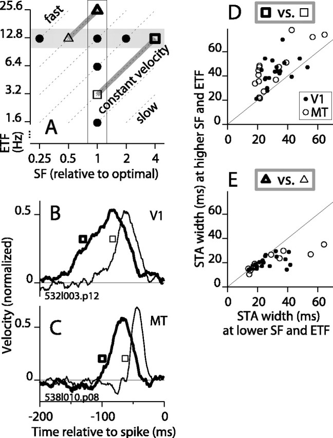
The temporal integration profile is not determined solely by stimulus velocity. A, The typical locations of stimuli in SF-TF space are plotted for our experiments in which ETF varied (white vertical band) and in which SF varied (gray horizontal band). Points are shown only for the highest five ETFs and only for SFs at full octave intervals. Diagonals are iso-velocity contours. The thick and thin open squares connected by the long gray line segment indicate, respectively, the stimulus at the highest SF and a velocity-matched stimulus at a lower SF and lower ETF. The shorter gray line segment connecting the thick and thin triangles shows a pair of velocity-matched stimuli at a faster speed. B, For a V1 cell, the STA is plotted for SF 1 cycle/degree and ETF 12.5 Hz (thick line) and SF 0.25 cycle/degree and TF 3.1 Hz (thin line). Thus, the velocity was 12.5°/sec in both cases. The thick and thin squares indicate the positions of the stimuli in the parameter space of A. C, For an MT cell, the STA is plotted for SF 4.60 cycles/degree and TF 12.5 Hz (thick line) and for SF 1.15 cycles/degree and TF 3.1 Hz (thin line). The velocity was 2.7°/sec in both cases. D, The width at half-height of the STA at the highest SF that produced a significant peak (thick square in A) is plotted against the STA width at the optimal SF tested at the same velocity (thin square in A). Nearly all points for V1 (filled circles) and MT (open circles) fell above the line. Two points for MT, one below the line and one above the line, fell outside the range shown here: (91, 113) and (115, 73). E, The STA width at the highest ETF (25 Hz) and the optimal SF (thick triangle in A) is plotted against the width at a lower ETF (typically 12.5 Hz) at the same velocity (thin triangle in A).

In summary, motion signals generated from patterns of high SF are integrated within a time window that is, on average, 20-30 msec wider than that for patterns of lower SF. This further supports the idea that individual DS neurons do not have fixed profiles of temporal integration.

Contrast and temporal integration

The luminance contrast of visual stimuli is known to affect temporal response properties in the visual system. For example, contrast influences the relative sensitivity to low and high TFs in retinal ganglion cells (Shapley and Victor, 1981), and it affects the phase of cortical simple-cell responses to drifting gratings (Dean and Tolhurst, 1986; Carandini and Heeger, 1994; Albrecht, 1995; Carandini et al., 1997). In addition, increasing contrast increases apparent velocity (Thompson, 1982), shortens reaction times to moving gratings (Burr and Corsale, 2001), and decreases psychophysically inferred integration times (Müller and Greenlee, 1998). We therefore examined the influence of contrast on motion integration in DS neurons by varying the contrast of the sinusoidal grating in our random motion stimulus while holding the SF at the optimal value for the cell and the ETF at 12.5 Hz.

For an example V1 cell, STAs are plotted in Figure 6A for four contrasts. The amplitude of the STA peak dropped rapidly with decreasing contrast, whereas the peak width changed very little. This behavior differed from that observed for the same cell when the speed (ETF) was reduced (Fig. 2A). Reducing the speed caused a marked widening of the STA, unlike reducing contrast, although both manipulations caused the firing rate to drop to near the spontaneous level. In a second example (Fig. 6B, MT cell), the amplitude also dropped with contrast, but the STA peak became substantially wider. Although the former example is from V1 and the latter from MT, the trends occurred equally in both areas. In ∼10% of cells in both V1 and MT, the STA peak first grew taller (as well as wider) as contrast dropped from 100% to ∼25-50%. Additional reductions in contrast caused a rapid decline in peak height.

Figure 6.

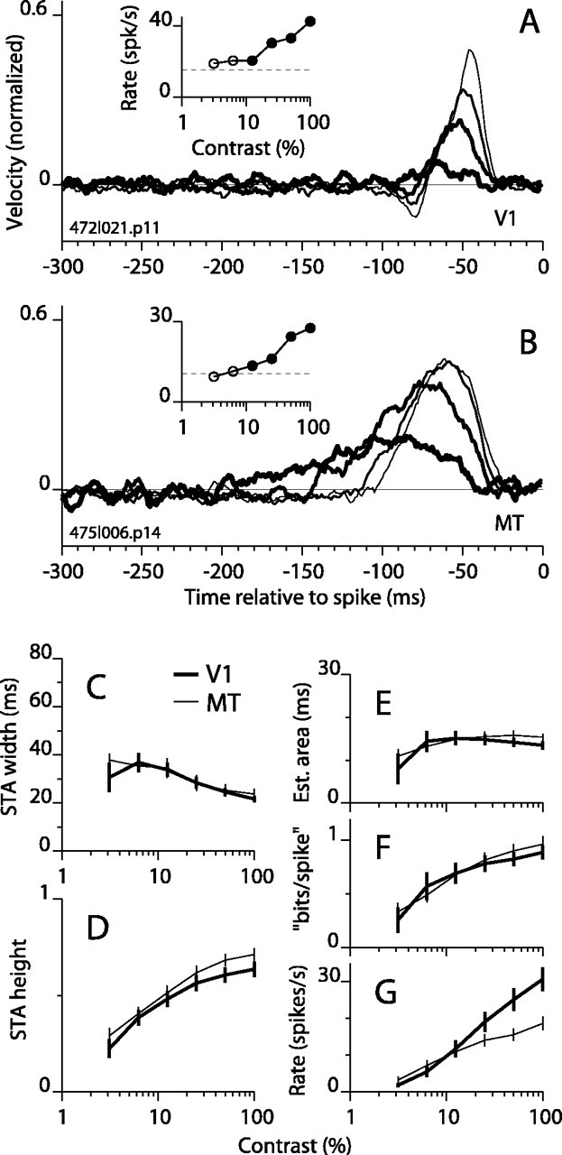
STAs as a function of grating contrast. The format is the same as in Figure 2, except that grating contrast is changing. A, STAs and firing rate for an example V1 cell. Only four of the six contrasts tested yielded STAs with significant peaks. As contrast was reduced from 100% to 12.5% (thinnest to thickest lines), the STA peak height decreased and became slightly broader. B, STAs and firing rates for an example MT cell. As contrast was reduced, there was a substantial broadening of the STA peak in addition to a decrease in amplitude. C-G, Same format as Figure 2, except horizontal axis is contrast.

On average, lower contrast was associated with wider (Fig. 6C) and shorter (Fig. 6D) STA peaks (26 V1 and 29 MT cells). This indicates that low-contrast stimuli, like slow moving or high SF stimuli, elicited responses in V1 and MT that reflected longer temporal integration. At low contrast, however, the increase in STA width was relatively modest and the decrease in height was relatively steep compared with the changes at low ETF or high SF (Figs. 2 and 3, respectively). This difference was also reflected in the plots of STA area, which had lower maximum values for contrast (Fig. 6E) than for ETF or SF (Figs. 2E, 3E). The mutual information per spike (Fig. 2G) decreased more rapidly with contrast than did area, because the information measure favors peak height over peak width. The distinctions between these trends and those for ETF and SF are made in a direct and quantitative manner below.

Comparing STA shapes across stimulus dimensions

To compare the changes in STA shape across ETF, SF, and contrast, we replotted the data from Figures 2, 3, and 6 in a parametric plot of STA height against width (Fig. 7A). The black lines represent the ETF data for V1 (thick line) and MT (thin line). The end points of these lines in the top left region of the plot, which corresponds to tall and narrow STAs, are the points for the highest ETF (fastest motion). As ETF decreased, the width of the STA increased and the peak height decreased; therefore, the data points trace a line from the top left to the bottom right of the plot. Sliding to the bottom right, each successive point corresponds to a one-octave drop in ETF. The end points in the bottom right region of the plot (low ETF) corresponds to short, wide STAs. Next, the gray lines show the progression of STA shape from high to low contrast (top and bottom end points are 100 and 3.125% contrast, respectively). The trend with contrast was different from that for ETF: the STA height dropped rapidly as contrast decreased but the width increased less than it did for low ETF.

Figure 7.

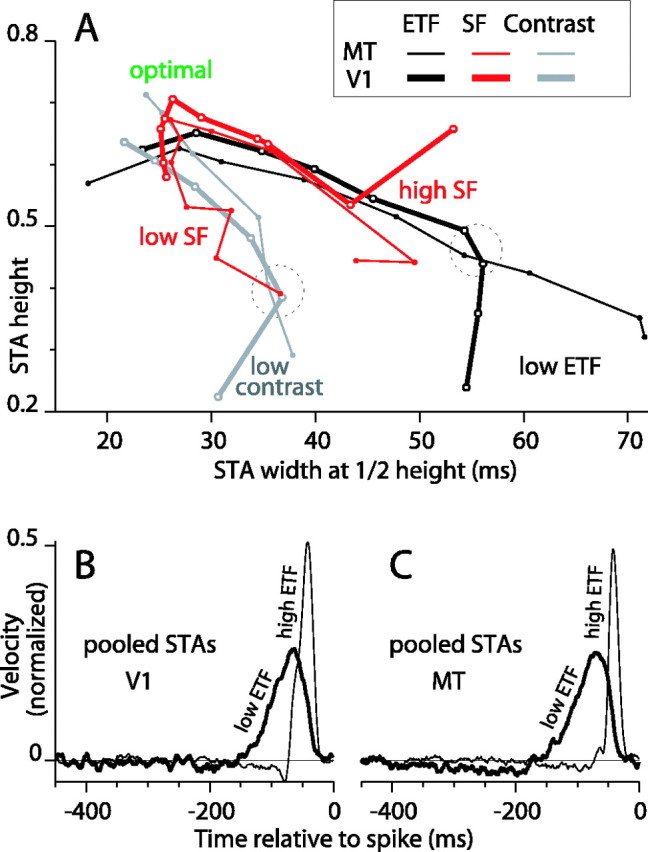
The effects on the STA shape of varying motion speed (ETF), grating SF, and grating contrast are compared. A, Data from Figures 2, 3, and 6 (C, D) are replotted in a parametric space of STA height versus width. Thick lines show data for V1 and thin lines for MT. Black lines show ETF data. Gray lines show contrast data. Red lines show SF data. Data are marked by points on lines. Low ETF marks the ends of the black lines that correspond to the slowest motion. Also labeled are the low contrast ends of the gray lines and the high SF and low SF ends of the red lines. The region marked optimal corresponds to the location of STAs for fast, high-contrast, and optimal SF stimuli. B, Database averages of the STAs for all 31 V1 complex DS cells for the two lowest ETFs (thick line) and the highest ETF (thin line). This demonstrates how the temporal profile of integration of the V1 population changes with stimulus speed. C, Averages like those in B are shown for all 21 MT cells. These averaged STAs show the dramatic change in temporal integration with motion speed for the population. It also reveals a weak negative lobe (from 200 to 400 msec before a spike) that was not easily observed in individual STAs.

Finally, in red are the data for SF, and both the low and high SF end points are labeled (Fig. 7A). As expected, the middle of the red curves, which correspond to optimal SFs, lies close to the second points on the black curves (for ETF, 12.5 Hz) and near the top points on the gray curves (100% contrast) because they all correspond to approximately the same stimulus parameters. The curves do not line up exactly (the cell populations are somewhat different, and there is noise in the parameter estimates), but they cluster closely in the region labeled “optimal.” Interestingly, the high-SF legs of the red curves followed approximately the course of the black curves toward low ETF, whereas the low-SF legs tended to follow the course of the gray curves toward low contrast. The latter trend was particularly evident for the MT data (thin red line).

It is important to consider that firing rate is lowered by four manipulations here: lowering the SF, raising the SF, lowering the contrast, and lowering the ETF (in fact, raising the ETF above 12.5 Hz also lowers the firing rate). However, these manipulations do not cause the STA to follow a single trajectory in the parameter space in Figure 7A. This strongly argues against the hypothesis that the signal strength at the soma of the recorded neuron controls temporal integration. If it did, then variations in contrast should be able to achieve STAs with shapes similar to those for variation in SF or ETF, but this was not the case. For example, the dashed circles in Figure 7A mark regions on the SF and ETF curves where the evoked firing rate is equal (∼6 spikes/sec above spontaneous) but STA width is different. The discrepancy between the firing rate and STA shape can also be seen for individual cells (e.g., within Fig. 2A, and between Figs. 2A and 6A, which show data from the same cell).

Across the parameter variations that we tested, the widest STAs occurred for low ETF stimuli, as indicated by the right end points of the black lines in Figure 7A. To show explicitly what the window of temporal integration looks like for DS cells operating at the slow end of their range, we averaged together the STAs for all V1 complex DS cells for the slowest two ETFs tested (0.1 and 0.2 Hz; no statistical criterion was applied to the STA peaks). The result is plotted in Figure 7B (thick line). This population STA reveals a window of positive temporal integration that extends over 120 msec, from ∼30 to 150 msec before the occurrence of a spike. The same type of population average for an ETF of 25 Hz (Fig. 7B, thin line) reveals a temporal profile spanning ∼45 msec, from 25 to 70 msec before the spike. Analogous population STAs are plotted for MT in Figure 7C. For slow motion, MT cells use information within a similar 120 msec window, but the population average also shows a clear depression that extends over at least 220 msec, from 180 to 400 msec before the spike. This suggests that slow antipreferred motion has a facilitatory effect on spiking that lasts for hundreds of milliseconds. Population averaging exposed the temporal extent of integration by removing noise in STAs for single cells, which by themselves rarely showed significant modulation this far back in time. The MT population STA for fast motion has a 30 msec window of temporal integration from 25 to 55 msec before the spike (Fig. 7C, thin line). It also has a negative lobe. Some caution is required when comparing these population averages to individual STAs because narrow STAs with large negative lobes can cancel positive portions of wider STAs. Nevertheless, the population averages for slow motion provide a less noisy look at integration at longer time scales.

The change in the STA over time

The different STA shapes observed across stimulus conditions show that the temporal integration of motion in V1 and MT cells is not fixed. However, the data presented reflect steady-state measurements (i.e., averages over the full duration of stimuli that lasted for 20-40 sec). We wondered whether changes in the STAs might reflect a slow adaptive process. To test this, we examined the width and height of the STAs computed from just the first 4 sec of the stimulus (the early period) and from a late period, 16-20 sec after stimulus onset. Windows shorter than 4 sec were impractical because they often yielded STAs that did not meet our criterion for a significant peak.

Figure 8 shows STAs in the early and late periods for slow and fast motion (ETF: 0.4 Hz at left, 25 Hz at right) for a V1 complex DS cell. The STA for the early period (Fig. 8A,C, thin solid lines) is somewhat narrower than the STA computed over the entire stimulus (dashed lines), whereas the STA for the later period (thick lines) was slightly wider. In Figure 8, we plotted the early STA width against the late STA width for individual cells for the slowest motion that yielded significant STA peaks (B) and for the fastest motion (D). The clusters of points for both V1 and MT were centered above the diagonal line, indicating that STAs in the late period were generally wider than those in the earlier period. The mean difference in width for slow motion was 9 msec for V1 (SD, 10; n = 29; p = 0.001; paired t test) and 7 msec for MT (SD, 12; n = 21; p = 0.08). For fast motion, the difference was 3 msec for V1 (SD, 5; n = 29; p = 0.02) and 4 msec for MT (SD, 7; n = 19; p = 0.14).

Figure 8.

Changes in the width of the STA peak over time during the stimulus. A, For an example V1 complex DS cell, the STA for ETF 0.4 Hz is plotted for the first 4 sec of the stimulus (thin solid line), for the 4 sec period beginning 16 sec after stimulus onset (thick line), and for the entire stimulus (dashed line). B, For each cell, the width at half-height of the STA peak for the late epoch is plotted against that for the early epoch for the lowest ETF that yielded a significant STA peak. Points for both V1 (filled circles) and MT (open circles) fell mainly above the diagonal line. C, D, The same format as A and B, except the comparison is made for fast motion (ETF 25 Hz).

We compared early and late STA widths for two other conditions that were associated with wider peaks: high SF and low contrast. For high SF, the width in the late period was, on average, larger by 5 msec in V1 (SD, 5 msec; n = 23; p = 0.001) and by 1 msec in MT (SD, 5 msec; n = 16; p = 0.53). For low contrast, the average width increased by 1 msec in V1 (SD, 9; n = 26; p = 0.81) and 3 msec in MT (SD, 10; n = 29; p = 0.19). We also tested the STA peak heights in all four conditions (fast, slow, high SF, and low contrast), but there were no significant changes, on average, between the early and late epochs. Evidence that our measurements were not dominated by noise is provided by the observation that in all conditions the early values were strongly correlated to the late values (0.75 < r < 0.96; p < 0.001 in all four cases for both width and height).

Although the mean increase in peak width in the late period was modest and, in many cases, not statistically significant, we tested whether the size of the increase over time was related to the size of the increase with stimulus parameters. For each cell, we paired the change in width across time with the change between the suboptimal (low ETF, high SF, or low contrast) and optimal conditions (the latter change being computed for full trials). In no case was there a significant correlation between these paired values, suggesting that the changes in width over time were not related to the changes across stimulus parameters. Finally, we found no significant correlation between the change in firing rate and the change in STA width during the trial.

In summary, integration time increased slightly, on average, during the trial for both wide and narrow STAs. We found no evidence to link the changes over time to the changes observed with stimulus parameters on a cell-by-cell basis. These results are consistent with the idea that changes in STA shape observed across stimulus parameters occurs predominantly on a time scale shorter than several seconds. However, better estimates of the rate of change of temporal integration may require a deterministic adapt-and-test paradigm that uses a test stimulus that is brief compared with the duration of the random input required for estimating the STA.

Frequency domain analysis of the STA

To facilitate the comparison of our results to the extensive frequency domain analysis of cortical RFs, we computed the FT of the STAs (see Materials and Methods) and plotted Fourier amplitude as a function of frequency. Here, we focus on the high-frequency cutoff and the distinction between low-pass and bandpass behavior, whereas in the time domain, we focused solely on the positive STA peak. We refer to an STA as bandpass if the amplitude of its FT fell below half of its maximum value at low frequencies. We expect narrower STAs to have higher cutoff frequencies and STAs with large dips (negative lobes to the left of the positive peak) to be bandpass.

Figure 9A shows the amplitude spectra for three of the STAs for the example cell from Figure 2A. For fast motion (ETF, 25 Hz) (Fig. 9A, thin line with dots), the STA spectrum is predominantly low-pass but drops somewhat at low frequency. For the slowest motion (ETF, 0.5 Hz) (Fig. 9A, thickest line), the spectrum is low-pass and the cutoff frequency (open circle) is substantially lower. Across the population at ETF 25 Hz, only 5 of 31 V1 cells (16%) and 6 of 21 MT cells (29%) were bandpass. All but one of these cells became low-pass at low ETFs. The average peak frequencies of the bandpass STAs were 11 and 13 Hz (SD, 1 Hz) for V1 and MT, respectively. For individual cells, the high-frequency cutoff for slow motion is plotted against that for fast motion in Figure 9B. The average cutoff frequency dropped from 19 to 6 Hz for V1 cells and from 21 to 7 Hz for MT cells as the stimulus ETF changed from its highest to its lowest value. This behavior in the frequency domain corroborates the large and systematic changes observed in the STAs in the time domain. A shift to lower frequencies in the temporal spectrum of the response may seem like a natural consequence of lowering the stimulus ETF; however, such a shift is not predicted by a standard model for motion detection (see below).

Figure 9.

Characterization of STAs in the frequency domain. A, For the example V1 cell in Figure 2A, the amplitude of the FT of the STA is plotted for ETF 0.2, 3.1, and 25 Hz (thick, medium, and thin lines, respectively). The open circles mark the cutoff frequency, defined to be the frequency at which the amplitude drops to half of the maximum value. B, The cutoff frequency for low ETF is plotted against that at ETF 25 Hz for V1 and MT cells (filled and open circles, respectively). The mean cutoff values for V1 (n = 31) were 6 Hz (SD, 2) and 19 Hz (SD, 5) for low and high ETF, respectively, and for MT (n = 21) were 7 Hz (SD, 3) and 21 Hz (SD, 10). C, For the example V1 cell in Figure 3A, the FT of the STAs are plotted for three SF values: 1.0, 2.0, and 7.9 cycles/degree (thin, medium, and thick lines, respectively). D, Cutoff frequency at high SF versus optimal SF for all cells. For V1 (n = 23), the mean cutoff dropped from 19 Hz (SD, 4) at the optimal SF to 10 Hz (SD, 5) at high SF. For MT (n = 18), the mean cutoff dropped from 21 Hz (SD, 9) for optimal SFs to 10Hz (SD, 5) for high SF. E, Cutoff frequency at low SF versus optimal SF. For V1, the mean cutoff was 14 Hz (SD, 5) at lowest SF. For MT, the mean cutoff was 13 Hz (SD, 7). F, For the example MT cell in Figure 6B, the FT of the STAs are shown for contrasts 12.5, 25, and 100% (thick, medium, and thin lines, respectively). G, Cutoff frequency at low contrast versus high contrast for all cells. The mean cutoffs at high contrast were 21 Hz (SD, 7) and 22 Hz (SD, 8) for V1 (n = 26) and MT (n = 29), respectively. At low contrast, the means were 10 Hz (SD, 5) and 11 Hz (SD, 4) for V1 and MT, respectively. For comparison, the thin line plots the mean values of the points from B.

Changes in stimulus SF caused consistent changes in the frequency domain across our population. At high and low SFs (Fig. 9C, thickest and thinnest lines), the STAs were low-pass and had high-frequency cutoffs that were typically lower than that at the optimal SF (medium line). At optimal SFs, the amplitude spectra tended to dip at low frequencies, but only 3 of 23 V1 cells and 4 of 18 MT cells qualified as bandpass. For individual cells, the consistency of the drop in cutoff frequency at high SF and at low SF relative to optimal SF can be seen in Figure 9, D and E (see legend for averages). These drops in cutoff frequency were not as large as those observed at low ETF.

The changes in the STA with contrast were well described as a leftward shift of the cutoff frequency at low contrast (Fig. 9F, thinnest and thickest lines show 100% and 12.5% contrast, respectively). For each cell, the cutoff frequency at the lowest contrast is plotted against that for 100% contrast (Fig. 9G). Cells with low cutoffs at high contrast (i.e., <∼20 Hz) had consistently low cutoffs, ∼4-8 Hz, at low contrast. However, cells with cutoffs >∼20 Hz at high contrast had more variable cutoffs at low contrast. This is apparent from the upward sweep and the vertical spread of points falling between 25 and 30 Hz on the x-axis in Figure 9G, which differs qualitatively from the trend for low versus high ETF in Figure 9B (thin line in G shows means at 5 Hz intervals for data in B). This suggests that the integration time in high TF channels is altered less by low contrast than by slow motion.

In summary, the cutoff frequencies of the STAs were consistently lower for slower motion, non-optimal SFs and lower-contrast stimuli. There was a mild trend for STAs at optimal parameters to show some bandpass behavior, but only a minority of cells actually qualified as bandpass. The presence of some bandpass cells is consistent with the existence of transient responses to sustained motion in MT (Lisberger and Movshon, 1999). However, the dominance of low-pass behavior is consistent with the results of Simpson (1994), who used a motion domain version of the two-pulse paradigm of Rashbass (1970) and found that the temporal integration of motion in human observers is primarily low-pass.

Modeling

Our experimental results indicate that the temporal integration profiles of DS cells vary with stimulus parameters, suggesting that a motion detector having a fixed temporal filter might not adequately describe the responses of DS cells. However, our analysis has focused on a particular aspect of the visual stimulus, namely, the one-dimensional signal describing its random motion over time, and we have neglected the raw visual stimulus, which is a sequence of images and thus a three-dimensional entity. The one-dimensional motion signal is uncorrelated in time and is therefore appropriate for computing the STA, whereas the luminance signal is correlated across time. The frequency spectrum of the luminance is low-pass with a cutoff frequency that becomes lower as the ETF drops (Eq. 19 and Fig. 12; see derivation in Appendix). This reflects the fact that the luminance at a particular spatial location changes more slowly for slower motion. It is reasonable to ask whether the widening of STA peaks is an inescapable result of the longer temporal correlation (of the luminance signal) at lower ETF.

Figure 12.

The power spectrum of the temporal modulation of luminance in our stimulus is plotted as a function of ETF. For the fastest motion (ETF 25 Hz), the spectrum is flat. For slower motion, the spectrum is low-pass, and the low-frequency cutoff decreases with ETF. See Equation 19 in the Appendix.

To test this, we simulated a mechanism that is commonly used in models of cortical motion processing, namely an ME model (Adelson and Bergen, 1985). A key component of this model is its set of spatiotemporal linear filters. Our implementation uses pairs of three-dimensional linear Gabor filters (Grzywacz and Yuille, 1990), in which the overall temporal profile is set by a Gaussian (Eq. 5). Each filter operates on the raw three-dimensional stimulus (a sequence of images in time) to produce a one-dimensional temporal response, which is then squared and summed for the pair. The result, known as ME, is tuned for direction of motion as well as for spatial and temporal frequency. To simulate the spiking response of a DS neuron, we let ME signals for the preferred and antipreferred directions control the excitatory and inhibitory conductances, respectively, of an IF model (see Materials and Methods). Parameters of the linear filters were set so that the direction tuning bandwidth, the optimal spatial and temporal frequencies, and the bandwidths of the latter were similar to a typical V1 complex DS neuron. Constants determining the offset and scaling of the synaptic conductances (Eqs. 11 and 12; see Materials and Methods) were set to provide a realistic range of firing rates as a function of stimulus contrast.

Using the optimal grating, we tested the model with the random motion stimulus at various ETFs and found that the STA peak height changed substantially but the width changed little as the ETF varied (Fig. 10A). The shape of the STAs remained similar to that of the Gaussian temporal envelope of the model (Fig. 10A, dashed gray line). The STAs are somewhat narrower than the Gaussian because of the squaring function in the model. Because the model is nonlinear, the STA does not represent an impulse response; nevertheless, it does reveal the window of temporal integration that was built into the model. We also tested the model over a full range of SFs and contrasts (data not shown) and found that the width of the STAs remained very close to that of the temporal Gaussian of the model. The ME model does not show changes in the STA because the model has no mechanism to extend its sensitivity further into the past, the way DS signals in V1 apparently do. The ME model operates on the stimulus with a fixed temporal weighting function that approaches zero very rapidly beyond the central region of its sensitivity; therefore, its output cannot possibly provide information about signals outside that time window in the face of any reasonable amount of noise.

Figure 10.

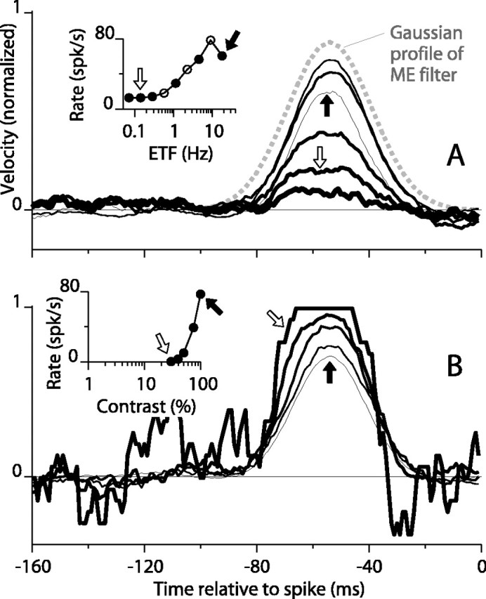
The STAs for a motion energy model change their height, but not their width, as ETF of the visual stimulus is changed. A, The same visual stimuli used in the experimental studies were input to a motion energy detector that drove an IF unit. The inset shows the mean firing rate as a function of ETF. STAs are shown in the main panel for ETFs marked by solid points in the inset. Arrows show correspondence of STAs and points in the inset. The dashed gray line plots the Gaussian function (SD, 15 msec) used to construct the linear filters for the motion detector. B, Response versus contrast for a reconfigured model in which contrast sensitivity was unrealistically low. For this regime, c_ex was 0.5 nS, and the mean of the additive noise (both n_p and n_a), was 0 (see Eqs. 11 and 12). All other parameters remained the same (see Materials and Methods). Thicker lines show STAs for lower contrast. Arrows mark correspondence between spike rates (inset) and STAs.

We did, however, observe some changes in the shape of the STA, mainly associated with changes in peak height, while testing a parameter regime of the model that had an unrealistically low-contrast sensitivity (Fig. 10B; see legend for parameter values). In this regime, in which the response at 50% contrast was only 13% of that at full contrast (Fig. 10B, inset), the STA peak grew taller with lower contrast (thicker curves). A few neurons behaved like this (the STA height increased initially as contrast decreased), but for the neurons, low contrast never caused the asymptoting of STAs observed for the model. Rather, this asymptoting behavior more closely matched the changes that we observed when we increased SF (Fig. 4). Additional testing of the model revealed that this behavior arose because of interactions between the statistics of the output of the ME mechanism and the properties of the IF mechanism. The best way to demonstrate how this occurs is to directly manipulate the input to the IF model without the encumbrance of the ME front end. We describe this below and show how to achieve STAs that grow substantially wider as stimulus parameters vary.

To test the IF model in isolation, we transformed the three-dimensional visual stimulus to a signal that could be given as input to the spike generator. This input signal was a time-varying conductance that took a value g_P during motion in the preferred direction and a value g_A during motion in the antipreferred direction, where g_P > g_A > 0. The signal, which resembled that in Figure 1C, was used to govern only the excitatory conductance, g_ex(t), of the IF model (Eq. 10; g_in was set to zero). This input can be conveniently parameterized by its mean, μ, and SD, σ, where μ = (g_P + g_A)/2 and σ = (g_P - g_A)/2. The use of conductances and the details of the IF model were not critical to achieve the results below. Indeed, we have used the same time-varying random stimulus sequences as input current injected into a model with Hodgkin-Huxley-like kinetics and as actual current injected into pyramidal neurons in slices of macaque visual cortex and have found behavior similar to that for the IF model (H. Oviedo and W. Bair, unpublished observations).

We examined the STAs for the IF model for sequences of input in which either the mean, μ, or the SD, σ, of the input varied. We also varied σ_noise, the SD of zero-mean Gaussian white noise (1 msec resolution) that was added to g_ex(t). In a low-noise regime (σ = 4 nS; σ_noise = 2 nS), varying μ from 6 to 40 nS caused significant changes in the STA width (Fig. 11A, thicker lines show STAs for lower μ). The STA peaks were wide and tall at low μ because threshold was crossed only after the consecutive occurrence of several preferred stimulus frames (i.e., 10 msec epochs of g_P). The peaks were narrower at higher μ because one preferred epoch was sufficient to reach threshold. At very high μ, both g_P and g_A were high, so the cell fired even for antipreferred stimuli, causing the STA peak to drop in amplitude (Fig. 11A, thinnest line).

Figure 11.

The shapes of STAs produced by an IF model depend on the mean and SD (μ and σ) of a random input. A, STAs from the IF model (see Materials and Methods) are shown for random binary inputs for μ from 24 to 40 nS (thicker lines indicate lower μ). The average firing rate is plotted against μ in the inset, where solid circles indicate values for which STAs are shown. The arrows mark the points and STAs for the lowest and highest means. The stimulus SD was 4 nS, and σ_noise was 2 nS. B, Increasing the additive Gaussian noise (σ_noise = 20 nS) caused the STAs to become narrower than those in A. The solid lines show STAs for the same μ and σ as in A (arrows and thickness indicate correspondence). STAs for three lower values of μ, which produced no spikes in the low noise regime in A, are shown as dashed lines (thicker dashed lines show lower μ). C, STAs are plotted for stimuli at SDs from 1 to 32 nS with μ = 16 nS and low additive noise (σ_noise = 2 nS). STA peaks were wider at lower SDs (thicker lines) than at high SDs (thinner lines). Arrows show correspondence between spike rate (inset) and STAs. D, Increasing the noise (σ_noise = 16 nS) caused the STAs to become narrower than those in C. The solid lines show STAs for the same μ and σ as in C (arrows and thickness indicate correspondence). STAs for three lower values of μ, which produced no spikes in the low noise regime in C, are shown as dashed lines (thicker dashed lines show lower μ).

The mechanism that increased the STA height at lower input levels here also caused the STAs to asymptote for the motion detecting model in Figure 10B, and it might underlie the asymptoting behavior in neurons (Fig. 4). However, the widening of the STA peaks here does not match the widening observed for the vast majority of neurons (Figs. 2A,B, 3A,B). The critical difference is that the STA peaks here grew to the asymptotic height before substantial widening could occur. We attempted to reduce the heights of wide STA peaks in the model by increasing σ_noise (20 nS) (Fig. 11B), but this also greatly reduced the peak width (Fig. 11A,B, compare thick lines marked by open arrows). We found that STA peaks could also be widened by decreasing σ while μ was constant (Fig. 11C), but again, adding noise reduced both the height and width of the peak (Fig. 11D; see legend for details).

We thoroughly explored the parameter range for our simplified, binary stimulus by testing the full grid of mean and SD values (at 2 nS resolution) that gave plausible mean firing rates (>0 and <200 spikes/sec). Under no conditions were we able to achieve wide STA peaks with low amplitudes, like those observed for most neurons. However, the observation that STA width can change as a result of changes in the input statistics to an IF spiking mechanism may provide a starting point for devising models that can account for changes in the STAs that match the data. For example, if randomly timed spikes could be added to the output spikes of the IF model, then the STA height would drop. This could be achieved by adding strong shot noise to the model that induced spikes regardless of the past stimulus movement or by adding a second stage to the model that integrated the IF spike trains with an independent signal. Such models could achieve what a single IF unit cannot: wide STA peaks with low amplitudes. This idea and some other possible mechanisms for adaptive temporal integration are considered in Discussion.

In summary, three important observations come from this modeling. First, the computations of a standard motion detector model are not responsible for the adaptive temporal integration observed for DS neurons. In particular, changes in the stimulus temporal frequency (i.e., changes in ETF) do not by themselves cause the STAs to change width. Second, the asymptoting of the STA peak height is consistent with a regime of operation in a spiking cell in which the signal/noise ratio of the input remains high while the maximum excursions of the input drop to near threshold (caused by a drop in either the input mean or variance). The cell becomes a peak detector in a low-noise regime and produces spikes that convey information about the stimulus with certainty (DeWeese et al., 2003). Finally, the nonlinearity of the IF mechanism provides a substrate for causing integration time to change, but not in a manner consistent with the bulk of our data.

Discussion

We found that the temporal integration profiles of V1 complex DS and MT cells changed substantially and in a similar manner in both cortical areas when spatial and temporal stimulus parameters were varied. We will use the general term “adaptive temporal integration” to refer to these changes and to the concept that temporal integration, or roughly speaking, the temporal RF of a neuron, is not fixed, but rather is stimulus dependent. Below, we will consider why the term “adaptive” may be warranted as we discuss our results for temporal frequency, SF, and contrast in terms of past physiological and psychophysical findings. Finally, we will consider the implications of adaptive temporal integration for neural coding and for the characterization and modeling of neuronal responses in the visual cortex.

TF and temporal integration

Varying the ETF, and thus the velocity, of the motion step in our stimulus caused the average STA half-width to change from 20 msec for fast motion to ∼60-70 msec for slow motion. This is perhaps best depicted by the population STAs for slow and fast movement shown in Figure 7, B and C. Strong modulation in the STA was usually confined within the epoch from 30 to 150 msec before the spike, but weaker modulation extended as far back as 200-400 msec in the MT population STA. The change in integration time correlated well with both TF and velocity, with neither value being the sole determining factor. Furthermore, such variation in the temporal profile is not predicted by standard motion detection models.

Previous studies of integration time in the visual cortex examined the phase of responses to drifting sinusoidal gratings as a function of TF (Hamilton et al., 1989; Albrecht, 1995; Hawken et al., 1996). These studies portrayed phase as a linear function of TF, which implies that integration time of a cell was fixed. If integration time is fixed for simple cells (the main focus of those studies), then adaptive temporal integration may arise from circuitry that is specific to complex DS cells. However, studies that modulated contrast with a sum of sinusoids found evidence for nonlinear temporal processing in cat area 17 (Dean et al., 1982; Reid et al., 1992). Reid et al. (1992) showed that integration time was shorter for broadband modulation and concluded, “the richer the stimulus, the faster the response.” Such a statement does not apply well in the motion domain, where moving a grating faster does not make the stimulus richer; however, in terms of luminance modulation, our fastest stimulus was indeed the most broadband. Thus, the changes that we observed with ETF and the results of Reid et al. (1992) may have a common origin involving changes in the distribution of luminance TF. However, “richness” would not account for changes with SF and contrast. Therefore, we propose that temporal integration in the cortex is controlled by a more general mechanism that responds to changes in a broad set of stimulus features, perhaps including any dimension along which neurons are tuned.

Another electrophysiological result that is consistent with our data is the inverse relationship between neuronal response latency and stimulus speed in MT (Movshon et al., 1990; Kawano et al., 1994; Lagae et al., 1994; Lisberger and Movshon, 1999; but see Raiguel et al., 1999). Although latency and integration time can, in principle, be independent, for many biological systems they are linked because simple low-pass filtering is associated with a delay. We have analyzed the response latency of this data set using the techniques described in Bair et al. (2002) and have found, not surprisingly, that stimulus conditions associated with longer integration time tend to be associated with longer onset latencies.

Most studies of the temporal integration of motion, however, have been psychophysical. Studies of short-range, or low-level, motion estimated the upper limit of temporal integration in two-flash apparent motion paradigms to be 80-100 msec (Braddick, 1973; Morgan and Ward, 1980; Baker and Braddick, 1985). These values are close to the upper limit of the span of modulation in our STAs, suggesting that they might be determined by constraints on DS signals within V1. Studies of continuous motion or multiframe apparent motion found similar temporal limits (McKee and Welch, 1985) and determined that temporal integration was longer for slower motion (Van Doorn and Koenderink, 1982; De Bruyn and Orban, 1988; Snowden and Braddick, 1991). Van Doorn and Koenderink (1982) identified a critical temporal value (above which rapid motion reversal was not perceived as such) that varied from 20 msec for fast motion to 50-80 msec for slow motion, which is very similar to the variations in STA width at half-height that we measured. Our data identifies an early point in the motion pathway in which a large proportion of such changes in temporal integration may arise.

The adaptive advantage of processing slower motion with a longer integration time is clear. Slower motion causes less change in the image and weaker signals in the visual system. Averaging over longer epochs can improve signal/noise ratio without sacrificing information.

SF and temporal integration

It has been known for decades that temporal integration in the human visual system is longer for high SF stimuli (Schober and Hilz, 1965; Nachmias, 1967; Vassilev and Mitov, 1976; Breitmeyer and Ganz, 1977), and recently it was suggested that this involves slower processing in cortical mechanisms tuned for high SF (Vassilev et al., 2002).

However, recent studies disagree about the relationship between temporal dynamics and SF in the cortex. Bredfeldt and Ringach (2002) reported that most V1 cells had higher SF preferences later in their response. Mazer et al. (2002), however, found that only a small fraction of cells showed this trend and argued that it could arise from latency differences between magno- (M) and parvocellular (P) signals. The results of the latter study stand in contrast to the large, systematic lengthening of integration time at high SF that we found for DS cells, which implies a shift to higher SF tuning later in the response. Our stimuli involved the prolonged presentation of a single SF, rather than the random interleaving of brief presentation (typically ≤20 msec) of various SFs (Bredfeldt and Ringach, 2002) or of various SFs and orientations (Mazer et al., 2002). Perhaps rapidly interleaved stimuli introduce large signals into the system that mask weaker signals associated with high SFs, thereby limiting the ability to resolve the response dynamics at high SF. Furthermore, the increase in integration time that we observed at high SF (∼25 msec, on average) is not likely to result from the relatively small differences in temporal properties of M and P cells (Hicks et al., 1983; Spear et al., 1994; Hawken et al., 1996; Maunsell et al., 1999; Levitt et al., 2001). The broad STAs at high SF in DS cells are not consistent with the high TF sensitivity and broad SF tuning of the lateral geniculate nucleus and therefore must reflect additional integration in V1.

An intriguing aspect of neuronal responses at high SF was the ability of some cells to signal preferred motion without false positives, as indicated by an increase in STA height. In the limit, a single spike indicated with certainty the direction of stimulus motion in a specified time period. We were able to reproduce this behavior by lowering the mean or the SD of the input to an IF unit under conditions of low additive noise. This gives some insight into the statistical structure of the local functional inputs that operate when the SF is relatively high for the cell. It suggests that the noise in the cell must be small relative to the signal required to cause a spike. This regime was particularly prominent in cells with low spontaneous rates, suggesting that it is not completely determined by the stimulus but also depends on properties intrinsic to the cell or its configuration within the network. Perhaps cells that are more hyperpolarized, receive more tonic inhibition, or are subject to inputs that are less noisy are those that have low spontaneous rates and operate in the high-threshold regime. Understanding why this tends to occur at high SF rather than low SF may provide insight into the mechanisms that underlie narrow SF tuning, a hallmark of the visual cortex (De Valois et al., 1982).

Having a longer integration time for high SF targets is consistent with course-to-fine processing in the visual system (Watt, 1987), but a bottom-up computational justification may be less clear. A high SF grating presented within a fixed RF region could arguably drive a greater number of non-overlapping subunits under the assumption of fixed SF bandwidth. Having more potential inputs would allow faster, not slower, integration.

However, the design of the cortex may not have anticipated sinusoidal grating patches, and longer integration might be desirable for small and detailed targets that would cause relatively weak signals.

Contrast and temporal integration

Lowering contrast lengthened the integration time for motion in complex DS and MT cells, which in the frequency domain amounts to a decrease in the high-frequency cutoff. The resulting shift is not likely to be caused by retinal contrast gain control (Shapley and Victor, 1981) because the latter involves mainly a change at low TFs, not a loss of response at high TFs. Nor is it likely to represent a shift between M and P inputs because M inputs are likely to dominate at low contrasts and are tuned to higher TFs. Parsimony suggests that the mechanisms involved are the same as those that create relative phase lags for gratings of lower contrast in simple cells (Dean and Tolhurst, 1986). Currently, there is no consensus regarding such a mechanism in the literature, which points to some combination of changes in membrane time constants caused by changes in conductance, short-term synaptic depression, and spike rate adaptation (Carandini and Heeger, 1994; Chance et al., 1998; Ferster and Miller, 2000; Kayser et al., 2001; Freeman et al., 2002). Our modeling suggests that the nonlinearity of thresholded spike generation can be added to this list.

In terms of computational advantage, it could be argued that increasing the integration time at lower contrast is needed to accommodate the lower signal/noise ratio associated with weaker signals. However, we found that lowering contrast was, on average, less effective at increasing integration time in DS cells than was lowering the speed of a high-contrast stimulus. This may be related to the idea that when movement is slow, longer integration risks nothing, but at low contrast, motion signals at any speed may still carry valuable information, some of which could be lost if temporal averaging became excessive.

The influence of contrast on response gain has been a major focus of the study of the optimization of visual processing for the visual environment (Shapley and Victor, 1981; Albrecht and Hamilton, 1982; Ohzawa et al., 1985; Sclar et al., 1989; Heeger, 1992; Carandini et al., 1997). However, such optimization should involve the control of response time course as well as gain and it should depend on stimulus features other than contrast. Our results suggest that contrast, SF, TF, and stimulus speed could all be factors in the control of temporal processing.

Comparing V1 to MT

We used the same types of stimuli to study temporal dynamics in V1 complex DS and MT cells, the latter being a known synaptic target of the former (Movshon and Newsome, 1996). We found only modest differences between these classes of cells. On average, MT cells seemed better able to integrate very slow motion. However, for a wide range of moderate to fast speeds, V1 cells had higher firing rates and, at any instant, conveyed more information, on average, per spike than did the MT cells. This is surprising because MT cells, having RFs 10 times wider than V1, on average, could potentially pool the signals from many V1 cells. The lower fidelity of MT cells suggests that they do not simply sum V1 responses but are designed for the integration of more complex patterns of motion (Movshon et al., 1985). Alternatively, MT could receive additional inputs related to higher processing or occulomotor states that reduce its apparent fidelity to the retinal optic flow. Under anesthesia, such additional signals could act as a source of noise in MT responses. Nevertheless, STAs for V1 complex DS and MT cells displayed mostly similar behavior, so it is possible that temporal profiles observed in MT arise from V1. Therefore, we focused on trying to understand adaptive temporal integration at the earlier stage.

Implications for spike coding

Two modes of spike encoding, perhaps at the ends of a continuum, were implied by the sequence of STAs produced as a stimulus parameter was varied from a value producing a high firing rate to a value producing a low firing rate. At one extreme, the STA peak dropped steadily with firing rate (Fig. 2A); at the other, the peak maintained its height (Fig. 2B) or increased in height (Fig. 4). The former is consistent with a signal sinking into noise, with many spikes having no direct relationship to the stimulus. The latter is consistent with the signal dropping below threshold but remaining above the noise such that the strongest excitatory events are the only ones that cause spikes (e.g., the high-threshold, low-noise regime of the IF model). From the point of view of the receiver, what distinguishes these regimes is the amount of information carried by a single spike. In the high-noise regime, individual spikes carry less information about the stimulus, whereas in the low-noise regime, they carry more. The low-noise regime was common enough across cells that at many suboptimal speeds and higher-than-optimal SFs the occurrence of a spike conveyed more information about direction than it did when elicited by an optimal stimulus. Perhaps the downstream circuitry uses some measure of mean rate over an appropriate population to set the weight assigned to spikes as stimulus conditions change.

The low-noise regime observed here under anesthesia is consistent with past observations of temporal modulation in MT of awake monkeys (Bair and Koch, 1996). In that study of responses to dynamic dot patterns, some cells had high firing rates with substantial rate modulation, whereas others fired isolated spikes at about the same time during the stimulus amid a baseline rate near zero (Bair and Koch, 1996, their Figs. 2 and 1, respectively). It is likely that the latter represented the low-noise regime described here.

Mechanisms for adaptive temporal integration

A standard motion detector constructed from a fixed set of filters did not account for the adaptive temporal integration that we observed. One possible explanation for our data involves a parallel model in which diverse spatiotemporal filters (Friend and Baker, 1993) feed into complex DS cells. A particular stimulus will match well only one set of input filters, and their temporal profile will be reflected in the response of the DS cell. However, parallelism might be unnecessary, and temporal integration may be altered along each serial pathway in which DS signals are generated. This could involve feedback or lateral signals, but it might be even simpler. For example, we tested how the STA of an IF unit changed as the statistics of its inputs changed. The nonlinearity of the IF unit was sufficient to cause a widening of the STA, but only after the STA had grown to its asymptotic height. Although this does not match the bulk of our data for complex DS cells, it is conceivable that such behavior could occur at an earlier stage (e.g., at spike generation in DS simple cells). This can be tested by recording from DS simple cells. Alternatively, the lengthening of integration time could occur in dendritic subunits in the complex DS cell themselves. There is growing evidence and interest in the idea that IF-like nonlinearities can occur in dendrites of cortical pyramidal cells. It is also possible that some of the other mechanisms mentioned above (changes in membrane time constants, synaptic depression, spike rate adaptation) could contribute to changes in integration time along the computational path for direction selectivity.

Implications for RF mapping and modeling

Regardless of mechanism, the substantial stimulus dependence of the temporal integration profile of DS neurons has important implications for how neurons are characterized and modeled. When mapping the spatiotemporal RF of visual neurons, which is now commonly done with random stimuli and reverse-correlation techniques analogous to those used here, it is critical to test how the resulting RF depends on the stimulus. Recent work has demonstrated that spatial profiles can also change significantly with stimulus contrast (Sceniak et al., 1999; Kapadia et al., 1999; Cavanaugh et al., 2002) and that auditory RFs can vary with the stimulus used to map them (Theunissen et al., 2000). It is possible that no single RF profile can be attributed to a cortical cell. This implies that models relying on a fixed filter to endow component neurons with their tuning properties could be highly inaccurate, in general. If we are to make models that are more generally useful for predicting responses to arbitrary time-varying stimuli, we must begin to identify the mechanisms that underlie adaptive changes in the spatial and temporal structure of neuronal RFs.

Appendix

In the motion domain, our random motion stimuli have power spectra that are flat up to their Nyquist frequency of 50 Hz (one-half of our 100 Hz frame rate). However, it is also important to consider their power spectra in the luminance domain. Here, we derive the temporal autocorrelation and power spectrum for our stimulus in the luminance domain.

The power spectrum of our random motion stimulus is a δ function in two-dimensional SF, because the stimulus is sinusoidal in space; therefore, we need only derive the TF spectrum. The stimulus moves in each time step by a fraction, 1/ρ, of the spatial cycle, where ρ = 2^m, m = 2,3,.. Because the stimulus is periodic, it occupies one of ρ states on each frame, the states being arranged on a circle with transition probabilities being one-half each to the counterclockwise and clockwise state. This cyclical random walk forms a Markov chain in which the transition probabilities, , of going from state j to k in n steps are described by Feller (1957):

13

where

14

and θ = e^i2π/ρ and q₀,..., q_ρ-1 are the transition probabilities from state 0 to states 0 through ρ - 1. In our case, q₁ = q_ρ-1 = 0.5 and all other q are 0, so Equation 13 reduces, as follows, to:

15

when (j - k + n) is even, and 0 otherwise.

These transition probabilities can be used to express the temporal autocorrelation function, A_τ = E[s_ts_t+τ], of the time-varying stimulus luminance, s_t, at any spatial location:

16

where x_j is the luminance of the stimulus in state j. Our stimulus is sinusoidal, so x_j = sin(2π j/ρ). Substituting Equation 15 with Equation 16 and simplifying yields the following:

17

For ρ = 4, A_τ is non-zero only at the origin, and for ρ > 4, it is a decaying exponential in time as follows:

18

where the time constant ϕ = -1/ln[cos(2π/ρ)]. The power spectrum, S_f, can be derived by taking the FT of the autocorrelation function (Bracewell, 1986). For ρ = 4, the spectrum is flat, and for ρ > 4, it is given by the following:

19

where f is temporal frequency. Figure 12 shows the power spectra for the nine ETFs that we used (i.e., for ρ = 4, 8, 16,..., 1024, where ETF = 100/ρ).

References

- Adelson EH, Bergen JR (1985) Spatiotemporal energy models for the perception of motion. J Opt Soc Am [A] 2: 284-299. [DOI] [PubMed] [Google Scholar]
- Albrecht DG (1995) Visual cortex neurons in monkey and cat: effect of contrast on the spatial and temporal phase transfer functions. Vis Neurosci 12: 1191-1210. [DOI] [PubMed] [Google Scholar]
- Albrecht DG, Hamilton DB (1982) Striate cortex of monkey and cat: contrast response function. J Neurophysiol 48: 217-237. [DOI] [PubMed] [Google Scholar]
- Albright TD, Desimone R (1987) Local precision of visuotopic organization in the middle temporal area (MT) of the macaque. Exp Brain Res 65: 582-592. [DOI] [PubMed] [Google Scholar]
- Bair W, Koch C (1996) Temporal precision of spike trains in extrastriate cortex. Neural Comput 8: 1185-1202. [DOI] [PubMed] [Google Scholar]
- Bair W, Cavanaugh JR, Movshon JA (1997) Reconstructing stimulus velocity from neuronal responses in area MT. In: Advances in neural information processing systems, Ed 9 (Mozer MC, Jordan MI, Petsche T, eds), pp 34-40. Cambridge, MA: MIT.
- Bair W, Cavanaugh JR, Smith MA, Movshon JA (2002) The timing of response onset and offset in macaque visual neurons. J Neurosci 22: 3189-3205. [DOI] [PMC free article] [PubMed] [Google Scholar]
- Baker Jr CL, Braddick OJ (1985) Temporal properties of the short-range process in apparent motion. Perception 14: 181-192. [DOI] [PubMed] [Google Scholar]
- Borghuis BG, Perge JA, Vajda I, van Wezel RJ, van de Grind WA, Lankheet MJ (2003) The motion reverse correlation (MRC) method: a linear systems approach in the motion domain. J Neurosci Methods 123: 153-166. [DOI] [PubMed] [Google Scholar]
- Bracewell RN (1986) The Fourier transform and its applications, Ed 2, revised. New York: McGraw-Hill.
- Braddick O (1973) The masking of apparent motion in random-dot patterns. Vision Res 13: 355-369. [DOI] [PubMed] [Google Scholar]
- Bredfeldt CE, Ringach DL (2002) Dynamics of spatial frequency tuning in macaque V1. J Neurosci 22: 1976-1984. [DOI] [PMC free article] [PubMed] [Google Scholar]
- Breitmeyer BG, Ganz L (1977) Temporal studies with flashed gratings: inferences about human transient and sustained channels. Vision Res 17: 861-865. [DOI] [PubMed] [Google Scholar]
- Buračas GT, Zador AM, DeWeese MR, Albright TD (1998) Efficient discrimination of temporal patterns by motion-sensitive neurons in primate visual cortex. Neuron 20: 959-969. [DOI] [PubMed] [Google Scholar]
- Burr DC, Corsale B (2001) Dependency of reaction times to motion onset on luminance and chromatic contrast. Vision Res 41: 1039-1048. [DOI] [PubMed] [Google Scholar]
- Carandini M, Heeger DJ (1994) Summation and division by neurons in primate visual cortex. Science 264: 1333-1336. [DOI] [PubMed] [Google Scholar]
- Carandini M, Heeger DJ, Movshon JA (1997) Linearity and normalization in simple cells of the macaque primary visual cortex. J Neurosci 17: 8621-8644. [DOI] [PMC free article] [PubMed] [Google Scholar]
- Cavanaugh JR, Bair W, Movshon JA (2002) Nature and interaction of signals from the receptive field center and surround in macaque V1 neurons. J Neurophysiol 88: 2530-2546. [DOI] [PubMed] [Google Scholar]
- Chance FS, Nelson SB, Abbott LF (1998) Synaptic depression and the temporal response characteristics of V1 cells. J Neurosci 18: 4785-4799. [DOI] [PMC free article] [PubMed] [Google Scholar]
- Cover TM, Thomas JA (1991) Elements of information theory. New York: Wiley.
- Dean AF, Tolhurst DJ (1986) Factors influencing the temporal phase of response to bar and grating stimuli for simple cells in the cat striate cortex. Exp Brain Res 62: 143-151. [DOI] [PubMed] [Google Scholar]
- Dean AF, Tolhurst DJ, Walker NS (1982) Non-linear temporal summation by simple cells in cat striate cortex demonstrated by failure of superposition. Exp Brain Res 45: 456-458. [DOI] [PubMed] [Google Scholar]
- DeAngelis GC, Ohzawa I, Freeman RD (1993) Spatiotemporal organization of simple-cell receptive fields in the cat's striate cortex. II. Linearity of spatial and temporal summation. J Neurophysiol 69: 1118-1135. [DOI] [PubMed] [Google Scholar]
- De Boer E, Kuyper P (1968) Triggered correlation. IEEE Trans Biomed Eng 15: 169-179. [DOI] [PubMed] [Google Scholar]
- De Bruyn B, Orban GA (1988) Human velocity and direction discrimination measured with random dot patterns. Vision Res 28: 1323-1335. [DOI] [PubMed] [Google Scholar]
- de Ruyter van Steveninck R, Bialek W (1988) Real-time performance of a movement-sensitive neuron in the blowfly visual system: coding and information transfer in short spike sequences. Proc R Soc Lond B Biol Sci 234: 379-414. [Google Scholar]
- De Valois RL, Albrecht DG, Thorell LG (1982) Spatial frequency selectivity of cells in macaque visual cortex. Vision Res 22: 545-559. [DOI] [PubMed] [Google Scholar]
- De Valois RL, Cottaris NP, Mahon LE, Elfar SD, Wilson JA (2000) Spatial and temporal receptive fields of geniculate and cortical cells and directional selectivity. Vision Res 40: 3685-3702. [DOI] [PubMed] [Google Scholar]
- DeWeese MR, Wehr M, Zador AM (2003) Binary spiking in auditory cortex. J Neurosci 23: 7940-7949. [DOI] [PMC free article] [PubMed] [Google Scholar]
- Emerson RC (1997) Quadrature subunits in directionally selective simple cells: spatiotemporal interactions. Vis Neurosci 14: 357-371. [DOI] [PubMed] [Google Scholar]
- Emerson RC, Bergen JR, Adelson EH (1992) Directionally selective complex cells and the computation of motion energy in cat visual cortex. Vision Res 32: 203-218. [DOI] [PubMed] [Google Scholar]
- Fahle M, Poggio T (1981) Visual hyperacuity: spatiotemporal interpolation in human vision. Proc R Soc Lond B Biol Sci 213: 451-477. [DOI] [PubMed] [Google Scholar]
- Feller W (1957) An introduction to probability theory and its applications, Vol 1, Ed 3. New York: Wiley. [Google Scholar]
- Ferster D, Miller KD (2000) Neural mechanisms of orientation selectivity in the visual cortex. Annu Rev Neurosci 23: 441-471. [DOI] [PubMed] [Google Scholar]
- Freeman TCB, Séverine D, Kiper DC, Carandini M (2002) Suppression without inhibition in visual cortex. Neuron 35: 759-771. [DOI] [PubMed] [Google Scholar]
- Friend SM, Baker Jr CL (1993) Spatio-temporal frequency separability in area 18 neurons of the cat. Vision Res 33: 1765-1771. [DOI] [PubMed] [Google Scholar]
- Gattass R, Gross CG (1981) Visual topography of striate projection zone (MT) in posterior superior temporal sulcus of the macaque. J Neurophysiol 46: 621-638. [DOI] [PubMed] [Google Scholar]
- Grzywacz NM, Yuille AL (1990) A model for the estimate of local image velocity by cells in the visual cortex. Proc R Soc Lond B Biol Sci 239: 129-161. [DOI] [PubMed] [Google Scholar]
- Hamilton DB, Albrecht DG, Geisler WS (1989) Visual cortical receptive fields in monkey and cat: spatial and temporal phase transfer function. Vision Res 29: 1285-1308. [DOI] [PubMed] [Google Scholar]
- Hawken MJ, Shapley RM, Grosof DH (1996) Temporal frequency selectivity in monkey visual cortex. Vis Neurosci 13: 477-492. [DOI] [PubMed] [Google Scholar]
- Heeger DJ (1987) Model for the extraction of image flow. J Opt Soc Am [A] 4: 1455-1471. [DOI] [PubMed] [Google Scholar]
- Heeger DJ (1992) Normalization of cell responses in cat striate cortex. Vis Neurosci 9: 181-197. [DOI] [PubMed] [Google Scholar]
- Hicks TP, Lee BB, Vidyasagar TR (1983) The responses of cells in macaque lateral geniculate nucleus to sinusoidal gratings. J Physiol (Lond) 337: 183-200. [DOI] [PMC free article] [PubMed] [Google Scholar]
- Hubel DH, Wiesel TN (1962) Receptive fields, binocular interaction and functional architecture in the cat's visual cortex. J Physiol (Lond) 160: 106-154. [DOI] [PMC free article] [PubMed] [Google Scholar]
- Kapadia MK, Westheimer G, Gilbert CD (1999) Dynamics of spatial summation in primary visual cortex of alert monkeys. Proc Natl Acad Sci USA 96: 12073-12078. [DOI] [PMC free article] [PubMed] [Google Scholar]
- Kawano K, Shidara M, Watanabe Y, Yamane S (1994) Neural activity in cortical area MST of alert monkey during ocular following responses. J Neurophysiol 71: 2305-2324. [DOI] [PubMed] [Google Scholar]
- Kayser A, Priebe NJ, Miller KD (2001) Contrast-dependent nonlinearities arise locally in a model of contrast-invariant orientation tuning. J Neurophysiol 85: 2130-2149. [DOI] [PubMed] [Google Scholar]
- Lagae L, Maes H, Raiguel S, Xiao D-K, Orban GA (1994) Responses of macaque STS neurons to optic flow components: a comparison of area MT and MST. J Neurophysiol 71: 1597-1626. [DOI] [PubMed] [Google Scholar]
- Levitt JB, Schumer RA, Sherman SM, Spear PD, Movshon JA (2001) Visual response properties of neurons in the LGN of normally-reared and visually-deprived macaque monkeys. J Neurophysiol 85: 2111-2129. [DOI] [PubMed] [Google Scholar]
- Lisberger SG, Movshon JA (1999) Visual motion analysis for pursuit eye movements in area MT of macaque monkeys. J Neurosci 19: 2224-2246. [DOI] [PMC free article] [PubMed] [Google Scholar]
- Liu RC, Tzonev S, Rebrik S, Miller KD (2001) Variability and information in a neural code of the cat lateral geniculate nucleus. J Neurophysiol 86: 2789-2806. [DOI] [PubMed] [Google Scholar]
- Maunsell JHR, Van Essen DC (1983) Functional properties of neurons in middle temporal visual area of the macaque monkey. I. Selectivity for stimulus direction, speed, and orientation. J Neurophysiol 49: 1127-1147. [DOI] [PubMed] [Google Scholar]
- Maunsell JHR, Ghose GM, Assad JA, McAdams CJ, Boudreau CE, Noerager BD (1999) Visual response latencies of magnocellular and parvocellular LGN neurons in macaque monkeys. Vis Neurosci 16: 1-14. [DOI] [PubMed] [Google Scholar]
- Mazer JA, Vinje WE, McDermott J, Schiller PH, Gallant JL (2002) Spatial frequency and orientation tuning dynamics in area V1. Proc Natl Acad Sci USA 99: 1645-1650. [DOI] [PMC free article] [PubMed] [Google Scholar]
- McKee SP, Welch L (1985) Sequential recruitment in the discrimination of velocity. J Opt Soc Am [A] 2: 243-251. [DOI] [PubMed] [Google Scholar]
- McLean J, Palmer LA (1989) Contribution of linear spatiotemporal receptive field structure to velocity selectivity of simple cells in area 17 of cat. Vision Res 29: 675-679. [DOI] [PubMed] [Google Scholar]
- McLean J, Palmer LA (1994) Organization of simple cell responses in the three-dimensional (3-D) frequency domain. Vis Neurosci 11: 295-306. [DOI] [PubMed] [Google Scholar]
- Merrill EG, Ainsworth A (1972) Glass-coated platinum-plated tungsten microelectrode. Med Biol Eng 10: 662-672. [DOI] [PubMed] [Google Scholar]
- Morgan MJ, Ward R (1980) Conditions for motion flow in dynamic visual noise. Vision Res 20: 431-435. [DOI] [PubMed] [Google Scholar]
- Movshon JA, Newsome WT (1996) Visual response properties of striate cortical neurons projecting to area MT in macaque monkeys. J Neurosci 16: 7733-7741. [DOI] [PMC free article] [PubMed] [Google Scholar]
- Movshon JA, Thompson ID, Tolhurst DJ (1978) Spatial summation in the receptive fields of simple cells in the cat's striate cortex. J Physiol (Lond) 283: 53-77. [DOI] [PMC free article] [PubMed] [Google Scholar]
- Movshon JA, Adelson EH, Gizzi MS, Newsome WT (1985) The analysis of moving visual patterns. Study group on pattern recognition mechanisms. Pontif Acad Sci Scr Varia 54: 117-151. [Google Scholar]
- Movshon JA, Lisberger SG, Krauzlis RJ (1990) Visual cortical signals supporting smooth pursuit eye movements. In: Cold Spring Harbor Symposia on Quantitative Biology, Vol LV, pp 707-716. New York: Cold Spring Harbor Laboratory. [DOI] [PubMed] [Google Scholar]
- Müller R, Greenlee MW (1998) Simultaneous discrimination of velocity and contrast of drifting gratings. J Opt Soc Am [A] 15: 2023-2035. [Google Scholar]
- Nachmias J (1967) Effect of exposure duration on visual contrast sensitivity with square-wave gratings. J Opt Soc Am [A] 57: 421-427. [Google Scholar]
- Nowlan SJ, Sejnowski TJ (1995) A selection model for motion processing in area MT of primates. J Neurosci 15: 1195-1214. [DOI] [PMC free article] [PubMed] [Google Scholar]
- Ohzawa I, Sclar G, Freeman RD (1985) Contrast gain control in the cat's visual system. J Neurophysiol 54: 651-667. [DOI] [PubMed] [Google Scholar]
- Parker AJ, Newsome WT (1998) Sense and the single neuron: probing the physiology of perception. Annu Rev Neurosci 21: 227-277. [DOI] [PubMed] [Google Scholar]
- Press HP, Teukolsky SA, Vetterling WT, Flannery BP (1992) Numerical recipes in C, the art of scientific computing, Ed 2. Cambridge, UK: Cambridge UP.
- Raiguel SE, Xiao D-K, Marcar VL, Orban GA (1999) Response latency of macaque area MT/V5 neurons and its relationship to stimulus parameters. J Neurophysiol 82: 1944-1956. [DOI] [PubMed] [Google Scholar]
- Rashbass C (1970) The visibility of transient changes of luminance. J Physiol (Lond) 210: 165-186. [DOI] [PMC free article] [PubMed] [Google Scholar]
- Reid RC, Soodak RE, Shapley RM (1987) Linear mechanisms of directional selectivity in simple cells of cat striate cortex. Proc Natl Acad Sci USA 84: 8740-8744. [DOI] [PMC free article] [PubMed] [Google Scholar]
- Reid RC, Soodak RE, Shapley RM (1991) Directional selectivity and spatiotemporal structure of receptive fields of simple cells in cat striate cortex. J Neurophysiol 66: 505-529. [DOI] [PubMed] [Google Scholar]
- Reid RC, Victor JD, Shapley RM (1992) Broadband temporal stimuli decrease the integration time of neurons in cat striate cortex. Vis Neurosci 9: 39-45. [DOI] [PubMed] [Google Scholar]
- Reid RC, Victor JD, Shapley RM (1997) The use of m-sequences in the analysis of visual neurons: linear receptive field properties. Vis Neurosci 14: 1015-1027. [DOI] [PubMed] [Google Scholar]
- Sceniak MP, Ringach DL, Hawken MJ, Shapley R (1999) Contrast's effect on spatial summation by macaque V1 neurons. Nat Neurosci 2: 733-739. [DOI] [PubMed] [Google Scholar]
- Schober HAW, Hilz R (1965) Contrast sensitivity of the human eye for square-wave gratings. J Opt Soc Am [A] 55: 1086-1091. [Google Scholar]
- Sclar G, Lennie P, DePriest DD (1989) Contrast adaptation in striate cortex of macaque. Vision Res 29: 747-755. [DOI] [PubMed] [Google Scholar]
- Shapley RM, Victor JD (1981) How the contrast gain control modifies the frequency responses of cat retinal ganglion cells. J Physiol (Lond) 318: 161-179. [DOI] [PMC free article] [PubMed] [Google Scholar]
- Simoncelli EP, Heeger DJ (1998) A model of neuronal responses in visual area MT. Vision Res 38: 743-761. [DOI] [PubMed] [Google Scholar]
- Simpson WA (1994) Temporal summation of visual-motion. Vision Res 34: 2547-2559. [DOI] [PubMed] [Google Scholar]
- Skottun BC, De Valois RL, Grosof DH, Movshon JA, Albrecht DG, Bonds AB (1991) Classifying simple and complex cells on the basis of response modulation. Vision Res 31: 1079-1086. [DOI] [PubMed] [Google Scholar]
- Snowden RJ, Braddick OJ (1991) The temporal integration and resolution of velocity signals. Vision Res 31: 907-914. [DOI] [PubMed] [Google Scholar]
- Spear PD, Moore RJ, Kim CBY, Xue J-T, Tumosa N (1994) Effects of aging on a primate visual system: spatial and temporal processing by lateral geniculate neurons in young adult and old rhesus monkeys. J Neurophysiol 72: 402-420. [DOI] [PubMed] [Google Scholar]
- Sutter EE (1987) A practical non-stochastic approach to nonlinear time-domain analysis. In: Advanced methods of physiological systems modeling, Vol 1 (Marmaerelis V, ed), pp 303-315. Los Angeles: University of Southern California. [Google Scholar]
- Theunissen F, Sen K, Doupe AJ (2000) Spectral-temporal receptive fields of nonlinear auditory neurons obtained using natural sounds. J Neurosci 20: 2315-2331. [DOI] [PMC free article] [PubMed] [Google Scholar]
- Thompson P (1982) Perceived rate of movement depends on contrast. Vision Res 22: 377-380. [DOI] [PubMed] [Google Scholar]
- Touryan J, Lau B, Dan Y (2002) Isolation of relevant visual features from random stimuli for cortical complex cells. J Neurosci 22: 10811-10818. [DOI] [PMC free article] [PubMed] [Google Scholar]
- Troyer TW, Krukowski AE, Priebe NJ, Miller KD (1998) Contrast-invariant orientation tuning in cat visual cortex: thalamocortical input tuning and correlation-based intracortical connectivity. J Neurosci 18: 5908-5927. [DOI] [PMC free article] [PubMed] [Google Scholar]
- Van Doorn AJ, Koenderink JJ (1982) Temporal properties of the visual detectability of moving spatial white noise. Exp Brain Res 45: 179-188. [DOI] [PubMed] [Google Scholar]
- Van Santen JPH, Sperling G (1984) Temporal covariance model of human motion perception. J Opt Soc Am [A] 1: 451-473. [DOI] [PubMed] [Google Scholar]
- Vassilev A, Mitov D (1976) Perception time and spatial frequency. Vision Res 16: 89-92. [DOI] [PubMed] [Google Scholar]
- Vassilev A, Mihaylova M, Bonnet C (2002) On the delay in processing high spatial frequency visual information: reaction time and VEP latency study of the effect of local intensity of stimulation. Vision Res 42: 851-864. [DOI] [PubMed] [Google Scholar]
- Watson AB, Ahumada AJ Jr (1983) A look at motion in the frequency domain. NASA Technical Memorandum 84352. ALSO: In Motion: perception and representation (Tsotsos JK, ed), pp. 1-10. New York: Association for Computing Machinery.
- Watt RJ (1987) Scanning from coarse to fine spatial scales in the human visual system after the onset of a stimulus. J Opt Soc Am [A] 4: 2006-2021. [DOI] [PubMed] [Google Scholar]
- Zeki SM (1974) Functional organization of a visual area in the posterior bank of the superior temporal sulcus of the rhesus monkey. J Physiol (Lond) 236: 549-573. [DOI] [PMC free article] [PubMed] [Google Scholar]