Discrimination of Voiced Stop Consonants Based on Auditory Nerve Discharges

Abstract

Previous studies of the neural representation of speech assumed some form of neural code, usually discharge rate or phase locking, for the representation. In the present study, responses to five synthesized CVC_CV (e.g., /dad_da/) utterances have been examined using information-theoretic distance measures [or Kullback-Leibler (KL) distance] that are independent of a priori assumptions about the neural code. The consonants in the stimuli fall along a continuum from /b/ to /d/ and include both formant-frequency (F1, F2, and F3) transitions and onset (release) bursts. Differences in responses to pairs of stimuli, based on single-fiber auditory nerve responses at 70 and 50 dB sound pressure level, have been quantified, based on KL and KL-like distances, to show how each portion of the response contributes to information coding and the fidelity of the encoding. Distances were large at best frequencies, in which the formants differ but were largest for fibers encoding the high-frequency release bursts. Distances computed at differing time resolutions show significant information in the temporal pattern of spiking, beyond that encoded by rate, at time resolutions from 1-40 msec. Single-fiber just noticeable differences (JNDs) for F2 and F3 were computed from the data. These results show that F2 is coded with greater fidelity than F3, even among fibers tuned to F3, and that JNDs are larger in the syllable final consonant than in the releases.

Introduction

Stop consonants like /b/ or /d/ are produced by stopping the flow of air in the vocal tract, either at the beginning or end of a syllable. Stops at the release of a syllable are characterized by a broadband burst of sound, followed by a vowel-like set of time-varying formants (the formant transitions) (Fig. 1). Stops at the closure of a syllable have only the formant transitions, in the opposite direction. The acoustic cues to the identity of stops have been defined in terms of the spectral characteristics of the burst and the formant transitions (Cooper et al., 1952; Delattre et al., 1955; Blumstein and Stevens, 1979; Kewley-Port, 1982; Smits et al., 1996). However, the spectra of stops depend on the context (i.e., the adjacent vowel). Invariant signatures that identify particular stops have not been found; instead, it seems that the auditory system can access many details of the spectrotemporal properties of a stop (Kewley-Port et al., 1983; Krull, 1990; Smits et al., 1996). Here, we consider the neural discrimination of the acoustic features of stops.

Figure 1.

Spectrograms of the five stimuli S1-S5. S1 and S5 are typical of the utterances /bab_ba/ and /dad_da/ in English; S2-S4 have the same vowel, but consonant properties are interpolated between /b/ and /d/. The spectrogram of S1 is shown for the whole stimulus (/bab_ba/), but only the first syllables of S2-S5 are shown (e.g., /dad/ for S5). The first three formant trajectories are highlighted with white lines. Note the burst of high-frequency energy at the release of the /d/ in S5 (arrow), which becomes weaker approaching S1. Spectrograms were computed from the first differences of the stimuli using a 25.6 msec Hamming window.

The peripheral neural representation of speech has been studied both for vowels (Sachs and Young, 1980; Delgutte and Kiang, 1984a; Conley and Keilson, 1995; Miller et al., 1997) and stop consonants (Miller and Sachs, 1983; Sinex and Geisler, 1983; Delgutte and Kiang, 1984b; Carney and Geisler, 1986). These analyses focused on the formant transitions and showed that the tonotopic representation of a stimulus reflects its spectra, formant energy peaks being signaled by peaks of response. These studies used either rate averaged over intervals of tens of milliseconds or longer or else strength of phase locking as the measure of response. Because psychophysical studies with speech (van Tasell et al., 1987, Shannon et al., 1995) suggest a role of speech envelope cues, it is likely that information about the stimuli is encoded by temporal patterns of spiking at intermediate time resolutions (e.g., 1-10 msec). This information, mainly reflecting the temporal envelope of the stimulus, is the focus here.

The response measure used here estimates the distance between the spike trains produced by a pair of stimuli. It is sensitive to all response differences down to a certain time scale. The “distance” between two spike trains is measured using a variant of the Kullback-Leibler (KL) distance, which can be related to the discriminability of the spiking patterns (Johnson et al., 2001). Differences in rate and differences in the pattern of spiking are both included in the measure, but phase-locking information is not, because of the choice of time scale.

Differences between the responses of auditory nerve (AN) fibers to the five stimuli shown in Figure 1 were computed. The results show a surprisingly strong representation of the release burst spectrum as well as the formants. There is significant information in the temporal pattern of spiking, beyond that encoded by rate; much of this information is carried by spike timing with a resolution of a few milliseconds.

Materials and Methods

Animal preparation and electrophysiology. All procedures were approved by the Johns Hopkins Animal Care and Use Committee (protocol CA99M255). Cats weighing 3-4 kg were anesthetized with xylazine (0.5 mg/kg, i.m.) and ketamine (20 mg/kg, i.m.), followed by atropine (0.1 mg, i.m.) to control secretions. Anesthesia was maintained with sodium pentobarbital (8-12 mg/hr, i.v., as needed to maintain areflexia). Temperature was maintained at ∼38.5°C. The trachea was cannulated, and the bulla was vented with a ≈1 m length of polyethylene tubing (PE-160) to prevent pressure buildup in the middle ear. The skull and dura were opened over the cerebellum, and the cerebellum was retracted medially to expose the AN. Glass micropipettes filled with 3 m NaCl (15-30 MΩ) were placed in the nerve where it exits the internal auditory meatus. Action potentials from single fibers were digitized with a Schmitt trigger and timed at a 10 μsec resolution.

Each fiber was characterized by its best frequency (BF) and threshold, determined with an automatic tuning-curve maker, and spontaneous activity. For analysis, fibers were separated into a low and medium spontaneous rate (LMSR) group and a high spontaneous rate (HSR) group at 18 spikes/sec.

Once classified, fibers were presented with the five stimuli shown in Figure 1; the stimuli were presented in an interleaved manner. Stimuli were repeated until contact with the fiber was lost (up to 300 repetitions). Data were always collected at 70 dB sound pressure level (SPL) (overall level of the vowel) and were sometimes also collected at 50 dB. Data were included in the analysis only if at least 80 repetitions of each stimulus were obtained.

Stimuli. For the neurophysiological experiments, five stimuli were used (Fig. 1). These are computer-synthesized two-syllable utterances of the form /CVC_CV/, where the vowel (V) was always /a/ as in “father” and the consonant (C) was a voiced stop similar to /b/ or /d/. The silence (_) between the syllables was 80 msec in duration. The consonants approximated /b/ in stimulus (S) 1, /d/ in S5, and were located along an intervening continuum for S2-S4. The stimuli were synthesized using the HLSYN speech synthesis system (version 2.2; Sensimetrics Corp.). S1 (/bab_ba/) and S5 (/dad_da/) were produced using standard parameters in the synthesizer. For S2-S4, the formant trajectories were interpolated linearly: starting frequencies of F2 were spaced at 0.2 kHz intervals between 0.9 (/b/) and 1.7 (/d/) kHz; starting frequencies of F3 were spaced at 0.2 kHz intervals between 2 and 2.8 kHz. F1 starting frequency was fixed at 0.5 kHz. The vowel formants were 0.72, 1.1, and 2.5 kHz. The formant transitions lasted 40 msec and the vowel 90 msec. The fundamental frequency of the voicing was fixed at 100 Hz.

At the release of the consonants, there was a short burst, followed ≈6 msec later by the beginning of voicing. The bursts for S2-S4 were generated by interpolating between the Fourier transforms of S1 and S5 bursts, which were obtained from the respective stimuli using a 26 msec window (Blumstein and Stevens, 1979). The interpolation was linear in decibels for the amplitude and linear for the phase. The stimuli were filtered with a human external ear transfer function (magnitude only), using a smooth version of the measurements of Wiener and Ross (1946) for a sound straight ahead. They were presented to the cat through a closed acoustic system consisting of a driver at the end of an earbar; typical calibrations for this system have been published previously (Rice et al., 1995). The stimulus at the cat's eardrum had approximately the same spectra in our closed acoustic system as at a human eardrum for free-field presentation of the same stimuli.

For the model calculations shown in Table 1, a set of 25 stimuli were synthesized having all possible combinations of the F2 and F3 starting frequencies found in S1-S5. Five of these stimuli are exactly S1-S5; the other 20 have different combinations of F2 and F3. These stimuli allow for information about F2 and F3 to be evaluated independently. The bursts were interpolated as for S1-S5. Model responses to these stimuli were computed using a computer model of AN responses (Zhang et al., 2001; Bruce et al., 2003).

Table 1.

Summary of JNDs (per fiber) computed from model responses with the 25 stimulus set

		JND (Hz)
Group of fibers	Formant	Release	Closure
BFs: 0.8-1.8 kHz	F2	60.0	145.2
	F3	223.2	354.0
BFs: 1.9-2.9 kHz	F2	68.7	137.9
	F3	78.8	129.2
BFs: 2.4-3.5 kHz	F2	72.7	96.1
	F3	75.3	107.6

Analysis. The goal of the analysis was to produce a measure of the difference between spike trains that can be related to their theoretical discriminability by an observer capable of using all the information in the spike train down to some time resolution Δ. The method is exactly that described by Johnson et al. (2001) in which an information-theoretic distance measure, the KL distance, is applied to distributions of spike times; the method is briefly described below.

The spike trains are binned into N bins of width Δ (1 msec for fibers with BFs ≥1 kHz, 2 msec for BFs between 0.5 and 1 kHz, 3 msec down to 0.33 kHz, etc., except for the data in Fig. 8). These binwidths were chosen to suppress timing information carried by phase locking. The number of spikes in bin b is R_b. The probability distributions for spikes in each bin are estimated from the data. This gives two sets of probability functions, P_A(R_b = r) and P_B (R_b = r), where A and B identify the stimuli; there is one such pair for each bin b. A measure of the difference between two such probability functions is the KL distance:

1

The KL distance is chosen because it quantifies the ultimate performance of an optimal classifier (e.g., a process that tries to estimate whether a spike train originated from stimulus A or B) (Cover and Thomas, 1991; Johnson et al., 2001). In fact, if the distributions are equal variance Gaussians (means, μ₁ and μ₂; variance, σ²), then the KL distance is proportional to the square of d'(defined as (μ_A-μ_B)/σ) (Green and Swets, 1966).

Figure 8.

Response distance declines at coarser temporal resolutions. Integrated distances during the release formant transition are plotted against the analysis time scale for different populations of fibers. The calculation of KL distance between spike count distributions was done as described in Materials and Methods, except that the binwidth (Δ) was set at 2, 4, 8, or 16 msec. The KL distance was integrated across time (0.03-0.07 sec) and across BF. Fibers were grouped in nonoverlapping 0.3 octave bins, distances were summed and normalized to the average in each bin, and then the bins were averaged, so the result plotted is average distance per fiber cumulated over 0.03-0.07 sec. A-C show cumulative distances for three BF ranges, as described in the figure titles. The sound level is indicated by the symbols, as defined in the legend.

If the bins are independent, then the KL distance for the joint probabilities of all the bins, or any subset of them, can be computed by adding the KL distances for the individual bins (Cover and Thomas, 1991). When there are serial dependencies between the bins, the KL distance must be computed from the joint probabilities of all B bins. This calculation requires a prohibitive amount of data, so Johnson et al. (2001) make the simplifying assumption that the dependencies can be modeled as a Markov process, in which the probability of a spike in bin b depends only on the occurrence of spikes in the previous D bins. Independent bins correspond to D = 0. With the Markov assumption,the joint probability function for the entire spike train can be written as a product of simpler functions:

2

The KL distance for a bin is defined as:

3

The cumulative KL distance is then the sum of these KL_AB(b) for b = D + 1... B plus the KL distance for the first D bins [i.e., between P_A(R₁, R₂,..., R_D) and P_B(R₁, R₂,..., R_D)]. Here, results are given for D = 0 and D = 4. For a binwidth Δ = 1 msec, D = 4 covers the major portion of refractoriness for most AN fibers (Li and Young, 1993). Because D is not known a priori, Johnson et al. (2001) recommend computing distances for increasing values of D until the values stabilize. For the AN, the results for D = 0 and 4 are essentially identical, as described in Results. Methods of estimating the quantities in Equations 2 and 3 were fully described by Johnson et al. (2001).

For Tables 1 and 2, estimates of the KL distance between the responses of populations of fibers are needed. These estimates are the sums of KL distances for the individual fibers, based on the assumption that individual fibers discharge independently, given the stimulus (Johnson and Kiang, 1976) (E. D. Young and M. B. Sachs, unpublished observations).

Table 2.

Summary of single-fiber JNDs computed from actual AN fiber responses, assuming that F2 fibers (BFs = 0.8−1.9 kHz) code for only F2 and F3 and higher BF fibers (BFs = 1.9−3.5 kHz) code equally for both F2 and F3

		JND (Hz)
Spontaneous rate	Sound level (dB SPL)	Release (1)	Closure	Release (2)	Formant	Actual number of fibers
High	70	183.1	368.9	192.3	F2	3600
	50	140.3	308.8	161.0
Low and medium	70	124.2	226.9	140.1	F2	2400
	50	93.7	230.9	104.3
High	70	228.5	399.8	235.5	F2, F3	3900
	50	319.1	498.5	283.4
Low and medium	70	301.0	426.9	322.9	F2, F3	2600
	50	435.6	776.0	483.6

The KL distance is asymmetric (KL_AB ≠ KL_BA). When there is a clear reference stimulus, as in just noticeable difference (JND) calculations, then this asymmetry is not a problem. When there is not, the so-called resistor average (RA) of the KL distances in the two directions is used, defined as 1/RA = 1/KL_AB + 1/KL_BA. The RA distance was computed after the accumulation of KL distances across time or fibers. The RA distance was used for the analysis of Figures 2, 3, 4, 5. KL distance is used for the JND calculations in Figure 9 and Tables 1 and 2. Also, KL distance is used in Figures 7 and 8, where we compare discriminability at different temporal resolutions, because of the relationship of KL distance with rate d'.

Figure 2.

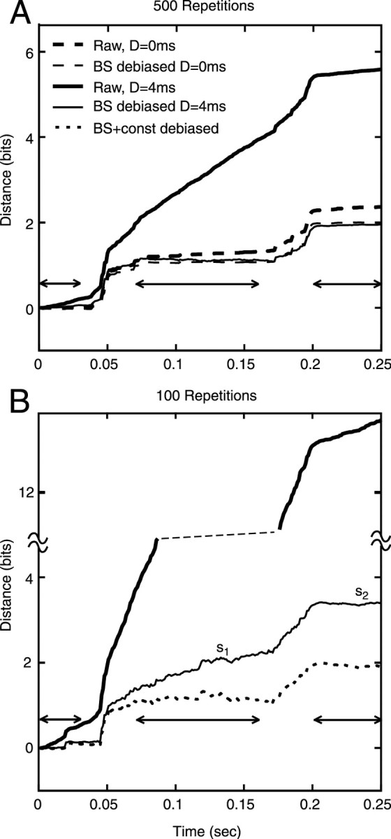
Cumulative raw and debiased RA distances between responses to S1 and S5 plotted versus time. The data were obtained from the model of Zhang et al. (2001) (Bruce et al., 2003). Only responses to the first syllable (/bab/ vs /dad/) are shown. Distance is plotted cumulatively on the y-axis (i.e., the distance at time t is the sum of the distances computed in all the bins from 0 to t). A, Data from 500 repetitions of the stimuli presented at 70 dB, for a model fiber with BF = 1.2 kHz and spontaneous rate = 100/sec. The analysis conditions are identified in the legend. Raw, Raw RA distance with no bias correction; BS, bootstrap correction. Results are shown for D = 0 and 4. B, Same plot for the first 100 responses from the same simulated data, for D = 4 only. Note that the ordinate is split at the dashed line.

Figure 3.

Responses to S1 and S5 and cumulative RA distance versus time for an AN fiber (BF = 1.7 kHz; spontaneous rate, 67.3/sec). A, B, PST histograms for the fiber in response to the two stimuli, computed with the same binwidth as the difference analysis (1 msec). Vertical lines demark the silences, consonants, and vowels for the full CVC_CV stimuli. C, Cumulative RA distance versus time for D = 0. The curves are identified in the legend. The dashed curves show the debiased difference ±1 SE. D. The same plots for D = 4. Now bootstrap debiasing leaves noticeable slopes (s₁, s₂, and s₃) during the vowels and inter-syllable silence). The dotted line shows the result of additional bias subtraction sufficient to make the slopes zero; this result is similar to the debiased result in C.

Figure 4.

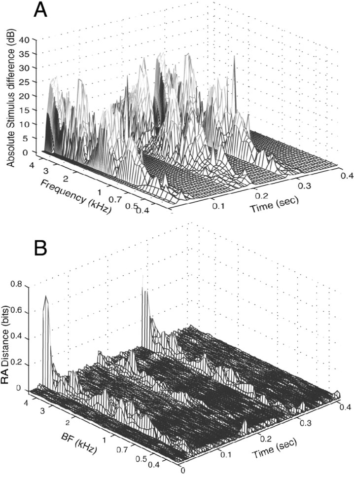
Three-dimensional plots of the differences between stimuli S1 and S5 and the RA differences between responses to those stimuli. A, Absolute value of the decibel difference between the spectrograms of S1 and S5; spectrograms were computed from the first-differences of the stimuli using a 25.6 msec Hamming window. Because of the first-differencing, the plotted amplitudes are approximately what they would be if stimulus power were grouped into logarithmic bins, as was done with the spike data. B, Debiased incremental RA distance between responses to S1 and S5 with D = 0. The average distance in each bin (e.g., Eq. 3 converted to RA distance but not cumulated across time) is plotted against time along the x-axis and fiber BF along the y-axis. Fibers are collected according to BF into overlapping 0.25 octave bins spaced every 0.0625 octaves. A fiber with BF b contributes to a bin with center frequency f with weight [1- log₂(b/f)/0.125]. The average KL distances were computed in this way and then converted to RA distances. Data are normalized by dividing by the sum of the weights in each bin, so the result is given as incremental RA distance per fiber. The number of fibers in each bin is shown in Figure 5C.

Figure 5.

Three-dimensional plots of debiased RA distances for various situations. A-D, Histograms of the number of fibers in each bin of the population plots in E-H. The BF axes at left are shared by the histograms and the three-dimensional color plots. E, Distances between responses to S1 and S5 at 70 dB (D = 0) for HSR fibers (spontaneous rate >18/sec). The plot is constructed in the same way as Figure 4, except distance is plotted on a color scale, shown at the bottom right. The white lines show the first three formants of the stimuli. The stimuli differ where the lines diverge, during the consonants, and response differences are seen mainly at those times. The formants are also different during the silences (before 0.05 sec and between 0.2 and 0.3 sec), but these differences are not conveyed in the stimuli and response differences are not seen in the silences. F, Distances between responses to S1 and S5 for LMSR fibers. The results are similar to those for HSR fibers. Because there are fewer LMSR fibers, there are several bins with no data (gray bars). G, Same plot for all the fibers; these are all the fibers in E and F and are the same data as in Figure 4. H, Debiased RA distances between responses to S1 and S2 at 70 dB. Distances are smaller than for S1 and S5.

Figure 9.

Debiased KL distances between responses of model fibers to the 25 stimulus set, with F2 and F3 varying independently. Distances are computed between the outer 24 stimuli and the center stimulus, for which F2 = 1.3 and F3 = 2.4 kHz. Distances were cumulated over 0.05-0.07 sec, and the x- and y-axes plot F2 and F3 formant frequency difference from the reference stimulus, at the center of the time window. A, Distances for 20 model fibers with BFs near F2 (0.8-1.8 kHz; spaced 0.06 octaves). Note that KL distance increases much more with changes in F2 than with F3. B, Distances for 20 model fibers with BFs near F3 (1.9-2.9 kHz; spaced 0.03 octaves). Here, KL distances increased with both F2 and F3. C, Distances for 20 model fibers with BFs between the upper half of the F3 region and to the low frequency end of the burst (2.4-3.5 kHz; spaced at 0.03 octave). Again, distances increased for both F2 and F3. Saturation is observed at the edges in B and C.

Figure 7.

Comparison of rate and response KL distances. A, Comparison of debiased KL distances between rates and the full KL distance measure, for the responses of fibers to S1 and S5, cumulated over the time interval 0.03-0.07 sec. The abscissa shows KL distances between the histograms of the spike counts over this time interval; the ordinate shows cumulated KL distance from the same time interval, using the method of Equation 3. Response distances were computed with D = 0 and debiased with bootstrapping. KL distance for rate was also debiased with bootstrapping. LMSR and HSR fibers are shown separately, as are responses at 50 and 70 dB. The line shows where distances are equal. B, PST histograms over 0.025-0.1 sec for one fiber in response to S1 and S5 at 70 dB (thin and thick solid lines) along with the cumulative KL distance between responses (dotted line) over the same interval. The fiber is marked by the arrow in A and has BF = 4.35 kHz, SR = 46.4/sec. The dashed lines show the average rates over 0.03-0.07 sec, which are essentially the same for the two stimuli.

The KL distance and, therefore, the RA distance is biased because random differences between two spike trains cumulate over the calculations. To estimate bias, the bootstrap method was used (Efron and Tibshirani, 1993). As described in Results, bootstrapping was not successful in fully removing bias with the number of repetitions available in our data for D = 4, although it did work for D = 0. We estimated the remaining bias in an ad hoc manner, from the rate of growth of RA difference during the vowels and silences in the stimuli. The RA difference should be zero during these times because the stimuli are identical (excluding the first 30 msec of vowel and silence, to remove the effects of adaptation). These bias estimates were used to remove the remaining bias, assuming that the bias is approximately the same during the vowel and consonant parts of the stimulus.

Computation of JNDs. If the probability function P_q(R) describes the distribution of a measured variable R as a function of parameter q, then the KL distance between P_q(R) and P_q+dq(R) is a measure of how easily q and q+dq can be discriminated on the basis of observing R. The SD of an estimator q̂ is a measure of the smallest distinguishable change in q (the JND); the smallest possible variance of an unbiased estimator q̂ is the Cramer-Rao bound, given by JND² = 1/F(q), where F is the Fisher information (Cover and Thomas, 1991). For small dq, Fisher information is related to KL distance as:

4

where KL is the KL distance between P_q(R) and P_q+dq(R). Using Equation 4, F(q) can be computed from a plot of KL versus dq. If q is a column vector of parameters, then KL = dq^T × F(q) × dq/2ln2, and the JNDs are given by the diagonal elements of the inverse of the Fisher information matrix, F^-1(q). For the results in Figure 8 and Table 1, F(q) was estimated from a plot of KL versus q = [F2, F3]^T (i.e., the parameters are the second and third formant frequencies at the start of the transitions). In this case, the coefficients f_ij of the matrix F must be chosen to fit the data on KL versus F2 and F3 as follows:

5

This estimation requires responses to the 25 stimulus set described above. It was not possible to obtain such data from AN fibers, therefore, spike trains were calculated using the model of Zhang et al. (2001) (Bruce et al., 2003). For the results in Table 2, Equation 4 was fit to plots of KL versus change in F2 for a subpopulation of fibers with BFs near F2, using the AN responses to S1-S5.

Results

Bias correction and serial dependence

To properly interpret the results, the bias in KL (or RA) distances has to be subtracted. The data contain an accurate check on bias correction in that the difference between the responses should be zero during the vowels and silences (i.e., when the stimuli are identical). Because the degree of serial dependence (D) was not known a priori, debiased difference measures were calculated at both D = 0 and 4 to determine empirically an appropriate value of D. With the number of stimulus repetitions available in our data, bias correction was found to be adequate for D = 0 but not for D = 4. Figure 2 shows an analysis of this situation using simulated spike trains produced by an AN model (Zhang et al., 2001; Bruce et al., 2003). Simulations are used here because a large number of stimulus repetitions can be obtained. The plots show cumulative RA distance (y-axis) plotted versus time during the first syllable only. The zero-difference periods (silence, vowel, and silence) are marked by horizontal arrows. Figure 2A shows results for 500 repetitions of the stimuli. Note that the raw (uncorrected) differences (thick solid and dashed lines) show substantial growth in distance during the vowel and silence; the growth is larger for D = 4. For 500 repetitions of the stimuli, bootstrapping eliminates the bias, as judged by the near-zero slopes of the bootstrap debiased distance (thin solid and dashed lines) during the vowel and silences. The final debiased distances are essentially the same for D = 0 and 4 msec.

When the analysis was done using only the first 100 repetitions of the same data (Fig. 2B), bootstrapping reduces, but does not eliminate, the bias for D = 4 (thin solid line); bootstrapping does eliminate the bias for D = 0 in this case (data not shown). Empirically, ∼80 repetitions are necessary for bootstrapping to work at D = 0. To estimate the unbiased distance in cases in which bootstrapping was insufficient, the bias was estimated from the slopes of the distance functions (Fig. 2B, s₁ and s₂) during periods in which the stimuli were identical (excluding the first 30 msec of the vowels and the silence, as explained in Materials and Methods). These bias estimates were then subtracted from the data. Because the amount of bias varies with the discharge rate, the bias is estimated separately for the silences and the vowels. No bias estimate is available during consonants, so the bias estimate from the vowels was used. This is clearly an approximation because the actual bias in the distance estimates depends on the rate of discharge of the fibers, which is significantly different during the consonant and the vowel. However, this method seems to work well in most cases. The dotted line in Figure 2B shows the result of additional debiasing using this slope rule. The final result is roughly the same as the successful bootstrap debiased estimates from the larger data set in Figure 2A.

Figure 3 shows responses to the stimuli and bias calculations for an AN fiber. Peristimulus time (PST) histograms of the responses of the fiber to S1 and S5 are shown in the top panels, and cumulative distances are plotted below. Bootstrap debiasing is sufficient for D = 0 (Fig. 3C, thick dashed line) but not for D = 4 (Fig. 3D, thick dashed line). The slopes s₁, s₂, and s₃ were used to subtract constant biases in this case, giving the dotted curve. Note that the result of bootstrap plus constant debiasing with D = 4 is about the same as the result of just bootstrap debiasing with D = 0, well within ± 1 SE (thin dashed lines). Both calculations give a cumulative distance across the whole stimulus of approximately three bits with gradual increases during the first and second consonants and a sudden large increase at ∼0.3 sec during the third consonant.

In both Figures 2 and 3, the final debiased distances did not change significantly with D; this was generally true. This result suggests that the effects of refractoriness are small compared with the noise in the estimates (reflected by the SE bounds in Fig. 3) and the distances that accumulate during times in which the stimuli are different (the jumps during the consonants in Figs. 2 and 3). For this reason, and the difficulties (large number of repetitions needed) of debiasing for D = 4, the calculations in the remainder of this report are done with D = 0 and with bootstrap debiasing alone.

Properties of RA distances

Debiased RA distances assuming independent bins (D = 0) were computed as in Figure 3 for a population of 238 AN fibers from 14 cats. The figures in this section show distances plotted against time and BF to show how the information about the differences between the stimuli distributes in the neural population.

Figure 4A shows the absolute difference between the spectrograms of S1 and S5 and, Figure 4B shows population RA distances between responses to the same stimuli at 70 dB. The incremental distance within each analysis time bin is shown instead of cumulating distance across time. Presenting the distances in this way emphasizes the location of informative changes in the neural response. Each BF bin shows the average distance across fibers gathered into logarithmically spaced 0.25 octave frequency bins. Within each BF bin, the average distance per fiber is shown as a function of time (x-axis). As expected, distances appear during the consonant portions of the stimuli, shown by the three ridges running parallel to the BF axis at the times of the consonants (∼0.03, 0.16, and 0.28 sec). During the vowels and silences, distances are small or nonexistent. The response differences are qualitatively similar to the stimulus differences in Figure 4A, in their behavior along the time axis. However, the distances vary considerably in size along the BF axis. The response distances are largest at high BFs, presumably reflecting the burst of energy at the release of the /d/ in S5 (Fig. 1, arrow). The response distances at the release are larger, relative to distances at lower BFs, than the corresponding differences in the stimuli (Fig. 4A). The distances are larger for the release consonants, at the beginning of the syllables (at 0.03 and 0.28 sec), than for the closure consonant at the end of the first syllable (at 0.16 sec). In part, this difference reflects the lack of a burst in the closure, but the difference is also seen at lower BFs, where the formant transitions are acoustically similar. The formant transitions are not easily seen in this plot.

Figure 5 shows population distances, as in Figure 4, on axes of BF (y-axis) and time (x-axis) with response distances shown by a color scale. The color scale is narrower than the z-axis scale in Figure 4, saturating at RA = 0.15 bits/msec fiber, to show details of the representation of the formant transitions. The histograms in Figure 5A-D show the number of fibers in each BF bin of the color plots. The distribution of fibers by BF is fairly uniform, except at low frequencies. However, because the stimulus differences are small at low frequencies (the F1 trajectory is identical in S1 through S5), the low number of low BF fibers does not affect the results. Response distances are shown for various populations of fibers, as described in the figure legends.

Significant response distances are seen during the consonants, when the formants (Fig. 5, white lines) are different. This is most clearly shown for the LMSR fibers in Figure 5F, where there is a triangular region of non-zero response distance that corresponds to the formant differences. The fact that differences are larger at release than at closure is evident, as is the large response distance in high BF fibers. The latter is especially evident in HSR fibers (Fig. 5E, white arrow); it is less apparent in the LMSR fibers because they do not respond as strongly because of their high thresholds.

Distances are larger as the stimulus differences become larger. The distances are much smaller for S1 versus S2 (Fig. 5H) compared with S1 versus S5 (Fig. 5G). Non-zero response distances for S1 versus S2 are seen mainly at and above the second formant. However, there is also a substantial difference in response at high BFs, reflecting the difference in the release burst spectrum at high frequencies, even though the burst is much weaker in S1 and S2.

In all cases, the response distances are smaller in the BF region near F3 than near F2. Presumably, this difference reflects the generally weaker neural representation of F3 relative to F2 (Miller and Sachs, 1983; Sinex and Geisler, 1983). This point will be more evident below when JNDs for formants are calculated.

Rate differences

The response distances shown in Figures 4 and 5 could be attributable to changes in spike rate or to changes in spike patterns (i.e., the temporal arrangement of spikes), or both. By rate, we mean the number spikes over a particular time interval (e.g., the duration of the formant transitions). Insight into this issue can be gotten by computing differences in the probability of spike occurrence, as shown in Figure 6A for S1 versus S5. Spike occurrence probability is expressed as instantaneous rate in 1 msec bins; fibers are binned and log-triangular smoothed along the y-axis as shown in the previous two figures to correspond with the response distance plots. Figure 6A contains similar information as in Figure 5G, except that positive and negative changes in spike occurrence are differentiated. Differences in spike occurrence probability are seen mainly during the consonants and are correlated with the differences between the formants. This is most clearly seen for F2, where the rate difference is positive for BFs near the F2 of S1 and negative for BFs near the F2 of S5. For F3, the changes in the spike occurrence probabilities are mostly negative, reflecting the fact that S1 has a lower amplitude than S5 in the F3 region, even at the F3 frequency. The high-frequency burst at consonant release is evident in Figure 6A, with a mixed pattern of negative and positive changes. The changes are larger for consonant release than closure, as for response distance measures.

Figure 6.

Rate differences and d′. A, Differences in spike occurrence probability, expressed as instantaneous rate differences in 1 msec bins, for responses to S1 minus S5 at 70 dB. Fibers are binned along the y-axis by BF as in previous figures. The differences are normalized to show change per fiber. The black lines show the trajectories of the first three formants. Differences are largest where the formants differ. B, d′ discriminability, computed (Eq. 6) from the difference in average rates over latencies of 0.03-0.07 sec (i.e., during the formant transition of the initial consonant). Each point is one fiber; the symbol identifies the spontaneous rate group of the fiber. The solid line shows a log-triangular smooth of the data points, as shown in Figures 4 and 5. The dashed horizontal lines show d′ = 0 and ±1.

Examination of Figure 6A shows that some differences in spike occurrence are maintained consistently over tens of milliseconds in most BF bins, which supports the idea that the difference in rate over tens of milliseconds is a large component of response distance. A change in spike pattern without a change in spike number would necessarily result in mixed positive and negative changes in Figure 6A, which is mainly seen at the burst frequencies (3.5-4.5 kHz).

The reliability of maintained rate changes for discrimination of the stimuli can be estimated by computing d′ for the average rate differences over 30-70 msec (i.e., during the formant transitions). Figure 6B shows d′ for the rate changes between S1 and S5, computed as:

6

where R_S1 and R_S5 are the average rates during the formant transitions of the first consonant and the σ²s are the associated variances. The calculation was done for each fiber individually, and the resulting d′s are plotted versus fiber BF in Figure 6B. The d′s are consistently large near the second formants of S1 and S5. Some units also showed large (negative) d′s across a wide range of higher BFs; these are mostly LMSR. The largest d's, mainly in LMSR fibers, have absolute values >1, so the task of discriminating S1 and S5 could be supported by the rate information in one of these fibers (Conley and Keilson, 1995; May et al., 1996).

Figure 6 shows that maintained rate differences provide reliable information about stimulus differences. However, there is additional information in the timing of spikes as suggested by the mixed positive and negative rate changes over shorter time intervals. Figure 7A shows a comparison of discriminability based on average rate change with discriminability based on the full response distance, both accumulated over a 40 msec interval. Each point shows data from one fiber. The abscissa shows the KL distance between histograms of the spike counts over 0.03-0.07 sec. This distance reflects only maintained rate changes. The ordinate shows the full KL distance measure cumulated over the same interval. Although there are many cases in which both response distance and rate difference are equally large, in general, the KL distances are substantially larger for response distance and there are many cases of substantial response distance with corresponding rate differences near zero. Thus, substantial information is encoded in the spike trains in terms of spike timing (i.e., changes in the arrangement of spikes on a 1 msec scale that do not necessarily lead to changes in average discharge rate).

Figure 7B shows the PST histograms of one case in which the response distance is large (∼5.9 bits) but the KL distance between rates is not (∼0.2 bits); this is the fiber marked by the arrow in Figure 7A. The average rates over the consonant period (164 and 182 spikes/sec; shown by the horizontal dashed lines) are roughly the same, but there is a substantial rearrangement of spikes during this time, indicated by the differences in the PST histograms. The cumulative response KL distance over the entire interval is plotted with the dotted line. Fibers that behaved like this were mainly HSR with high BFs or low spontaneous rate (LSR) with low BFs, and this behavior was seen mainly at 70 dB SPL. The opposite case, fibers with approximately equal KL distance for spike count and response distances (Fig. 7A, symbols along the straight line), was mainly LSR fibers for data collected at the 50 dB SPL stimulus level.

Effects of time resolution

The results in Figure 7 show that there is significant information in the temporal arrangement of the spikes. To investigate the degree of temporal resolution needed to extract that information, the calculation was repeated with several binwidths (Δ), from 1 to 16 msec. Debiased KL distances between responses to S1 and S5 were cumulated across the formant transition time (0.03-0.07 sec) and averaged across populations of fibers in three BF ranges. Figure 8 shows that KL distance decreases with binwidth in all cases. For the whole population (BFs between 0.33 and 5 kHz) (Fig. 8A), the values are about the same at both sound levels. However, for BFs in the formant transition range (0.76-3.3 kHz) (Fig. 8B), distances are larger at 50 dB, presumably because of saturation of rate changes at the higher level. Finally, at higher BFs (3.3-5 kHz) (Fig. 8C), the situation is reversed, and there is substantially more information at 70 dB. In this case, the responses are mainly to the energy in the burst, which was near or below threshold for many fibers at 50 dB.

Computation of JNDs for F2 and F3

The KL distances can be used to estimate JNDs for discrimination of stimuli, using the approach based on the Fisher information described in Materials and Methods. This calculation allows analysis of the relative quality of the representations of F2 and F3 in different groups of fibers. The approach is to fit Equation 5 to data on KL distance versus F2 and F3. Because F2 and F3 do not vary independently in the stimulus set S1-S5, responses to the larger 25 stimulus set described in Materials and Methods are needed. Because it is not feasible to obtain sufficient data from AN fibers for this number of stimuli with enough repetitions for the debiasing to work, responses generated by a model of the AN were used (Zhang et al., 2001; Bruce et al., 2003). Responses were generated for HSR fibers spaced at 0.03 or 0.06 octave intervals; 250 repetitions of each of the 25 stimuli were presented at 70 dB. Debiased KL distances (D = 0) were computed between the central stimulus (which is S3, with starting frequencies of F2 = 1.3 and F3 = 2.4 kHz) and the 24 other stimuli.

Figure 9 shows the distances between the central stimulus and each of the others for fibers with BFs near F2 (Fig. 9A), fibers with BFs near F3 (Fig. 9B), and fibers with BFs in the top half of the F3 region, up to the beginning of the high-frequency burst (Fig. 9C). The distances were cumulated over 0.05-0.07 sec, to keep the changes in F2 and F3 small, consistent with the assumption that dq is small in Equations 4 and 5. Using this time interval also removes the effects of the burst, the characteristics of which are not directly determined by F2 and F3. In the F2 region (Fig. 9A), the KL distance plot has a trough-like shape parallel to the F3 axis, showing that distance grows mainly with changes in F2; F3 has little effect on these fibers. In contrast, KL distance for fibers in the F3 region and above (Fig. 9B,C) has a bowl shape, saturating at the edges, so that KL distance grows almost equally with both F2 and F3. This is consistent with previous results showing, for vowels, that fibers with BFs near F2 respond primarily to F2, whereas fibers with BFs near F3 respond to several stimulus components (Young and Sachs, 1979; Miller et al., 1997).

The surfaces in Figure 9 were fit with Equation 5 to estimate the elements of the Fisher matrix F, and JNDs for F2 and F3 were computed as the square roots of diagonal elements of F^-1. Because the edges are saturated, the fitting was done to the central nine points. Furthermore, the fits are only approximate as the surfaces in Figure 9 are not perfectly parabolic as expected from Equation 5. The KL distances in Figure 9 are summed across 20 fibers in each of the populations. Inspection of Equations 4 and 5 shows that the ultimate JND varies inversely with the square root of the number of independent fibers. F2 and F3 JNDs in Table 1 were calculated for a single equivalent fiber that provides information equal to the average across the 20 original fibers. The approximate number of fibers in the cat auditory nerve in those three frequency ranges are 3600, 2100, and 2700 (Liberman, 1982, Keithley and Schreiber, 1987), so the JNDs predicted for the whole populations would be smaller than the values in Table 1 by the square roots of these values. Results are shown in Table 1 for both the release (0.05-0.07 sec) and closure (0.16-0.18 sec) consonants. As expected from the shape of Figure 9A, the F3 JNDs are significantly larger than the F2 JNDs for the fibers with BFs near F2. For the F3 fibers and the above-F3 fibers, the two JNDs are close in size. As expected from Figures 4 and 5, the JNDs are smaller for the release consonant than for the closure. There is a substantial amount of F2 and F3 information in fibers above the F3 region (as depicted by the surface of Fig. 9C and JNDs in the bottom row of Table 1), primarily because of differences in the spectrum levels of the stimuli above F3. Although the highest frequency region (3-3.5 kHz) does not contain formant energy, the level there changes systematically with the F2 and F3 starting formant frequencies, so it contributes to theoretical discriminability.

Estimates of the F2 and F3 JNDs can also be made from the real fiber data by assuming that fibers with BFs near F2 encode F2 only and fibers with BFs near F3 encode both F2 and F3 equally. Thus, for stimuli in which both F2 and F3 vary (as in S1-S5), the KL distances in the F2 region (0.8-1.8 kHz) can be attributed wholly to F2 changes, and KL distances in the F3 region and above (1.9-3.6 kHz) can be split equally between F2 and F3. In this way, KL distances caused by changes in F2 and F3 can be estimated, and Equation 4 can be fit to one-dimensional plots of KL distance versus change in either F2 or F3. The calculation was done separately for the LMSR and HSR fibers at both 70 and 50 dB. Table 2 shows the JNDs calculated in this way for two populations of fibers: (1) F2 JNDs for fibers with BFs near F2 (0.8-1.9 kHz); and (2) F2 or F3 JNDs for fibers with BFs near and above F3 (1.9-3.5 kHz). Again, JNDs are expressed for one fiber, which conveys the average information across the population. The JNDs for the whole populations can be computed by dividing by the square roots of the numbers of fibers in the right column of Table 2. The overall JND for F2 can be computed by combining results from the two AN populations. Those come out to be ∼2-12 Hz.

Per fiber, JNDs are smaller at release than at closure in all cases and are approximately equal for the two releases. For F2, the LMSR fibers provide smaller JNDs than HSR fibers; however, for F3, the opposite is true. Presumably, this reflects the fact that the stimulus level is lower in the F3 frequency region, so that HSR fibers are less saturated for BFs near F3 than for BFs near F2. This hypothesis is supported by the fact that JNDs get larger with sound level in the F2 region but smaller in the F3 region.

Although the model gives qualitatively similar results as the actual data, comparison of the F2 JNDs in Tables 1 and 2 shows that JNDs in the model are substantially smaller than those in the data. This probably results from the fact that the model underestimates the degree of suppression of F2 responses by F1 (Bruce et al., 2003), so that the F2 representation in the model is less contaminated by F1 responses than in the data.

Discussion

Representation of stop consonants

Previous work on the neural representation of stop consonants focused on the formant transitions. AN fibers provide a tonotopic representation of the spectrum of the transition period, in which the movement of the formants is represented by a moving maximum of response among fibers, the BFs of which correspond to the formant frequency (Miller and Sachs, 1983; Sinex and Geisler, 1983). Given those results, it was expected that differences in the neural responses to two stops would be observed as in Figures 3, 4, 5. The computed response distances show five patterns: (1) distances are larger for fibers with BFs near the transitions (Figs. 5, 6); 2) distances differ between LMSR and HSR fibers depending on stimulus level (from the JNDs in Tables 1 and 2); (3) distances are larger for larger stimulus differences (Figs. 5G,H, 9); (4) distances are larger at release than at closure (Fig. 5; Tables 1 and 2); and (5) differences are larger for the bursts than for the formant transitions (Fig. 4).

The strong representation of the release burst was unexpected. Our results suggest that the burst provides good information for the discrimination of stops, even for S1 and S2 at the /b/ end of the stimulus continuum where the burst is weak (Fig. 5H). Because of their short duration, bursts are a relatively small part of the overall stop consonant signal, even though their spectrum levels are a few decibels louder than the rest of the stop onset (Stevens and Blumstein, 1978). For voiced stops (/b, d, g/ in English), the formant transitions are sufficient to identify the stop; bursts improve performance but are often weak cues by themselves (Stevens and Blumstein, 1978). However, for unvoiced stops (/p, t, k/ in English) and for some consonant-vowel combinations with voiced stops (e.g., “front” vowels like /i/), the burst may be quite important (for review, see Smits et al., 1996). Regardless, the neural representations studied here show a strong representation of the burst. Certainly, the burst response is strong, in part because the burst is preceded by silence in a release stop; because of the silence, AN fibers are released from adaptation, which can substantially shape the responses to consonants by decreasing responses of fibers at BFs in which preceding sounds have significant energy (Delgutte and Kiang, 1984b). This effect is probably also responsible for the stronger representation of the formant transitions at release compared with closure.

JNDs for formant frequencies

When corrected for the total number of fibers in the population, the JNDs in Tables 1 and 2 are considerably smaller than JNDs measured in human observers, which are typically ∼100-200 Hz for similar stimuli (Porter et al., 1991; van Wieringen and Pols, 1995). This difference is frequently reported in attempts to predict psychophysical limens from AN data, in that a small number of fibers is often sufficient for discrimination in quiet for a broad range of different auditory discriminations (Siebert, 1968; Viemeister, 1983; Young and Barta, 1986; Winslow and Sachs, 1988; May et al., 1996).

In the present case, the JND predictions are optimistic because they assume the ability to compare stimuli with perfect timing synchronization. Such synchronization can be assumed if the optimal processor has the stimulus onset time from the onset burst of spikes in fibers like the example in Figures 3,A and B, and 7B. For stops, such a burst occurs for most BFs and SR of fibers and could be communicated across BFs to synchronize processing.

One clear prediction of the data are that the JNDs for formant change should be smaller at release than at closure. This result is consistent with some data (Sidwell and Summerfield, 1986) but is inconsistent with other work (van Wieringen and Pols, 1995). The JNDs for formant frequency extent in the latter study vary significantly, depending on the duration of the syllable, the number of other formants included in the stimulus, and the details of the timing of the formant transitions. Thus, the nature of the discrimination task for formant transitions is complex and is likely to be affected by factors other than the raw discriminability of the neural representations, such as masking interactions with the vowel and categorical perception of natural-sounding consonants.

The nature of the auditory stimulus representation

The method used here measures the differences between responses to stimuli, instead of estimating the actual representation, and allows systematic analysis of the sensitivity of the representation to different aspects of the stimulus. More important, it allows identification of the locus of that sensitivity in time and place in the population (Johnson et al., 2001; Samonds et al., 2003). Thus, in Figure 9, it is clear that the representation of F2 and F3 is rather different in the F2 versus F3 neurons. In neurons with BFs near F2, the representation provides little information about F3, whereas in neurons with BFs near F3, both F2 and F3 are represented. This difference is consistent with the inferences from direct studies of the neural representations of both vowels (Young and Sachs, 1979; Miller et al., 1997) and stops (Miller and Sachs, 1983; Sinex and Geisler, 1983), in which a corresponding result has been obtained by studying the phase-locking of AN fibers to the F2 and F3 components of the stimulus.

Typically, analyses of neural representations of auditory stimuli have been based on the average discharge rate over the whole stimulus or on phase locking to the stimulus waveform. The former is primarily an estimate of the ability of cochlear tuning to resolve the stimuli spectrally, in that the average rate of a neuron is determined mainly by the amount of energy passing through its tuning curve. Phase locking provides more detailed information about the stimulus components to which the neuron responds. Phase locking clearly provides information in situations in which discharge rate alone does not (Keilson et al., 1997; Miller et al., 1999). The method used here provides a systematic way to analyze the information carried by fluctuations in the response of a fiber at intermediate time scales, down to 1 msec, not including phase locking.

The temporal information revealed in Figure 7 is not a temporal code for the stimulus, in the sense of the temporal codes found in cortical neurons, in which the pattern of spiking is unrelated to the stimulus waveform (Richmond and Optican, 1987; Middlebrooks et al., 1994). Instead, the spiking patterns studied here are determined by the stimulus envelope, and the neurons provide a representation of that envelope (Delgutte et al., 1998). In fact, the population RA distance plots (Fig. 5) show large distances at times corresponding to the period of the stimulus (where the envelope peaks). These occur as striations in the incremental RA distances across time, which are more evident when the stimulus differences are small (Fig. 5E-G, F3 region, H) and at lower levels of stimulus presentation (50 dB SPL; data not shown). The incremental RA distances between responses of a fiber to two stimuli show significant correlation with the absolute envelope differences between the stimuli (after filtering with a tuning curve-like filter); this effect can be seen qualitatively in Figure 7B. It is well known that information can be extracted from the temporal fluctuations of the speech signal, independent of spectral information. Rosen (1992) divides the temporal information into envelope (modulations at 2-50 Hz), periodicity (modulations from 50-500 Hz), and fine structure at higher frequencies. The envelope encodes fluctuations in amplitude produced by the sequence of phonemes and syllables in the speech; periodicity information is important for voicing, voice pitch, stress, and intonation. Fine structure conveys information about the spectral content of the signal. On the time scale considered here, between the time resolution of 1 msec and the average rate-integrating window of 40 msec (Figs. 6, 7), the temporal fluctuations relate to periodicity. Inspection of Figure 7B suggests that the differences relate mainly to fluctuations in the amplitude of the voiced signal from period to period.

The analysis method

Measures of neural selectivity based on KL distance show considerable bias, which must be removed for proper interpretation. The amount of data required to remove bias is the main difficulty in applying this technique. An essential aspect of the debiasing process here is the presence of identical stimulus control times, which were used to evaluate the adequacy of the debiasing calculation. An important result here is that serial dependency does not affect the distance measures, for the AN fibers studied. This was shown using simulations (Fig. 2), in which sufficient data can easily be obtained, and by using an ad hoc debiasing technique with real data (Fig. 3). In both cases, the distance measure was the same, regardless of the degree of serial dependence assumed (D = 0 or 4 msec). This result allowed serial dependence to be ignored, which made bootstrap debiasing possible. This result probably derives from the near-Poisson nature of AN spike trains (Johnson, 1996). In fact, AN fibers have an absolute refractory period of ∼1 msec and a relative refractory period that can last for 20 msec or more (Johnson and Swami, 1983; Miller and Mark, 1992; Li and Young, 1993). Apparently, the relative refractory effects are not large enough to substantially change the distance calculations. Note that the lack of serial dependence does not hold in models of neurons in lateral superior olive (Johnson et al., 2001) or in ensembles of neurons in visual cortex (Samonds et al., 2003).

References

- Blumstein SE, Stevens KN (1979) Acoustic invariance in speech production: evidence from measurements of the spectral characteristics of stop consonants. J Acoust Soc Am 66: 1001-1017. [DOI] [PubMed] [Google Scholar]
- Bruce IC, Sachs MB, Young ED (2003) An auditory-periphery model of the effects of acoustic trauma on auditory nerve responses. J Acoust Soc Am 113: 369-388. [DOI] [PubMed] [Google Scholar]
- Carney LH, Geisler CD (1986) A temporal analysis of auditory-nerve fiber responses to spoken stop consonant-vowel syllables. J Acoust Soc Am 79: 1896-1914. [DOI] [PubMed] [Google Scholar]
- Conley RA, Keilson SE (1995) Rate representation and discriminability of second formant frequencies for /e/-like steady-state vowels in cat auditory nerve. J Acoust Soc Am 98: 3223-3234. [DOI] [PubMed] [Google Scholar]
- Cooper FS, Delattre PC, Liberman AM, Borst JM, Gerstman LJ (1952) Some experiments on the perception of synthetic speech sounds. J Acoust Soc Am 24: 597-606. [Google Scholar]
- Cover TM, Thomas JA (1991) Elements of information theory. New York: Wiley-Interscience.
- Delattre PC, Liberman AM, Cooper FS (1955) Acoustic loci and transitional cues for consonants. J Acoust Soc Am 27: 769-773. [Google Scholar]
- Delgutte B, Kiang NYS (1984a) Speech coding in the auditory nerve: I. Vowel-like sounds. J Acoust Soc Am 75: 866-878. [DOI] [PubMed] [Google Scholar]
- Delgutte B, Kiang NYS (1984b) Speech coding in the auditory nerve: IV. Sounds with consonant-like dynamic characteristics. J Acoust Soc Am 75: 897-907. [DOI] [PubMed] [Google Scholar]
- Delgutte B, Hammond BM, Cariani PA (1998) Neural coding of the temporal envelope of speech: relation to modulation transfer functions. In: Psychophysical and physiological advances in hearing (Palmer AR, Rees A, Summerfield AQ, Meddis R, eds), pp 595-603. London: Whurr.
- Efron B, Tibshirani RJ (1993) An introduction to the bootstrap. Boca Raton, FL: Chapman and Hall/CRC.
- Green DM, Swets JA (1966) Signal detection theory and psychophysics. New York: Wiley.
- Johnson DH (1996) Point process models of single-neuron discharges. J Comput Neurosci 3: 275-299. [DOI] [PubMed] [Google Scholar]
- Johnson DH, Kiang NYS (1976) Analysis of discharges recorded simultaneously from pairs of auditory nerve fibers. Biophys J 16: 719-734. [DOI] [PMC free article] [PubMed] [Google Scholar]
- Johnson DH, Swami A (1983) The transmission of signals by auditory-nerve fiber discharge patterns. J Acoust Soc Am 74: 493-501. [DOI] [PubMed] [Google Scholar]
- Johnson DH, Gruner CM, Baggerly K, Seshagiri C (2001) Information-theoretic analysis of the neural code. J Comput Neurosci 10: 47-69. [DOI] [PubMed] [Google Scholar]
- Keilson SE, Richards VM, Wyman BT, Young ED (1997) The representation of concurrent vowels in the cat AVCN: evidence for a periodicity-tagged spectral representation. J Acoust Soc Am 102: 1056-1071. [DOI] [PubMed] [Google Scholar]
- Keithley EM, Schreiber RC (1987) Frequency map of the spiral ganglion in the cat. J Acoust Soc Am 81: 1036-1042. [DOI] [PubMed] [Google Scholar]
- Kewley-Port D (1982) Measurement of formant transitions in naturally produced stop consonant-vowel syllables. J Acoust Soc Am 72: 379-389. [DOI] [PubMed] [Google Scholar]
- Kewley-Port D, Pisoni DB, Studdert-Kennedy M (1983) Perception of static and dynamic acoustic cues to place of articulation in initial stop consonants. J Acoust Soc Am 73: 1779-1793. [DOI] [PMC free article] [PubMed] [Google Scholar]
- Krull D (1990) Relating acoustic properties to perceptual responses: a study of Swedish voiced stops. J Acoust Soc Am 88: 2557-2570. [DOI] [PubMed] [Google Scholar]
- Li J, Young ED (1993) Discharge-rate dependence of refractory behavior of cat auditory-nerve fibers. Hear Res 69: 151-162. [DOI] [PubMed] [Google Scholar]
- Liberman MC (1982) The cochlear frequency map for the cat: labeling auditory-nerve fibers of known characteristic frequency. J Acoust Soc Am 72: 1441-1449. [DOI] [PubMed] [Google Scholar]
- May BJ, Huang A, Le Prell G, Hienz RD (1996) Vowel formant frequency discrimination in cats: comparison of auditory nerve representations and psychophysical thresholds. Aud Neurosci 3: 135-162. [PMC free article] [PubMed] [Google Scholar]
- Middlebrooks JC, Clock AE, Green DM (1994) A panoramic code for sound location by cortical neurons. Science 264: 842-844. [DOI] [PubMed] [Google Scholar]
- Miller MI, Mark KE (1992) A statistical study of cochlear nerve discharge patterns in response to complex speech stimuli. J Acoust Soc Am 92: 202-209. [DOI] [PubMed] [Google Scholar]
- Miller MI, Sachs MB (1983) Representation of stop consonants in the discharge patterns of auditory-nerve fibers. J Acoust Soc Am 74: 502-517. [DOI] [PubMed] [Google Scholar]
- Miller RL, Schilling JR, Franck KR, Young ED (1997) Effects of acoustic trauma on the representation of the vowel /e/ in cat auditory nerve fibers. J Acoust Soc Am 101: 3602-3616. [DOI] [PubMed] [Google Scholar]
- Miller RL, Calhoun BM, Young ED (1999) Discriminability of vowel representations in cat auditory-nerve fibers after acoustic trauma. J Acoust Soc Am 105: 311-325. [DOI] [PubMed] [Google Scholar]
- Porter RJ, Cullen JK, Collins MJ, Jackson DF (1991) Discrimination of formant transition onset frequency: psychoacoustic cues at short, moderate, and long durations. J Acoust Soc Am 90: 1298-1308. [DOI] [PubMed] [Google Scholar]
- Rice JJ, Young ED, Spirou GA (1995) Auditory-nerve encoding of pinna-based spectral cues: rate representation of high-frequency stimuli. J Acoust Soc Am 97: 1764-1776. [DOI] [PubMed] [Google Scholar]
- Richmond BJ, Optican LM (1987) Temporal encoding of two-dimensional patterns by single units in primate inferior temporal cortex. II. Quantification of response waveform. J Neurophysiol 57: 147-161. [DOI] [PubMed] [Google Scholar]
- Rosen S (1992) Temporal information in speech: acoustic, auditory and linguistic aspects. Philos Trans R Soc Lond B Biol Sci 336: 367-373. [DOI] [PubMed] [Google Scholar]
- Sachs MB, Young ED (1980) Effects of nonlinearities on speech encoding in the auditory nerve. J Acoust Soc Am 68: 858-875. [DOI] [PubMed] [Google Scholar]
- Samonds JM, Allison JD, Brown HA, Bonds AB (2003) Cooperation between area 17 neuron pairs enhances fine discrimination of orientation. J Neurosci 23: 2416-2425. [DOI] [PMC free article] [PubMed] [Google Scholar]
- Shannon RV, Zheng FG, Kamath V, Wygonski J, Ekelid M (1995) Speech recognition with primarily temporal cues. Science 270: 303-304. [DOI] [PubMed] [Google Scholar]
- Sidwell A, Summerfield Q (1986) The auditory representation of symmetrical CVC syllables. Speech Commun 5: 283-297. [Google Scholar]
- Siebert WM (1968) Stimulus transformations in the peripheral auditory system. In: Recognizing patterns (Kollers A, Eden M, eds), pp 104-133. Cambridge: MIT.
- Sinex DG, Geisler CD (1983) Responses of auditory-nerve fibers to consonant-vowel syllables. J Acoust Soc Am 73: 602-615. [DOI] [PubMed] [Google Scholar]
- Smits R, ten Bosch L, Collier R (1996) Evaluation of various sets of acoustic cues for the perception of prevocalic stop consonants. I. Perception experiment. J Acoust Soc Am 100: 3852-3864. [DOI] [PubMed] [Google Scholar]
- Stevens KN, Blumstein SE (1978) Invariant cues for place of articulation in stop consonants. J Acoust Soc Am 64: 1358-1368. [DOI] [PubMed] [Google Scholar]
- Van Tasell DJ, Soli SD, Kirby VM, Widin GP (1987) Speech waveform envelope cues for consonant recognition. J Acoust Soc Am 82: 1152-1161. [DOI] [PubMed] [Google Scholar]
- van Wieringen A, Pols LCW (1995) Discrimination of single and complex consonant-vowel- and vowel-consonant-like formant transitions. J Acoust Soc Am 98: 1304-1312. [Google Scholar]
- Viemeister NF (1983) Auditory intensity discrimination at high frequencies in the presence of noise. Science 221: 1206-1207. [DOI] [PubMed] [Google Scholar]
- Wiener FM, Ross DA (1946) The pressure distribution in the auditory canal in a progressive sound field. J Acoust Soc Am 18: 401-408. [Google Scholar]
- Winslow RL, Sachs MB (1988) Single-tone intensity discrimination based on auditory-nerve rate responses in backgrounds of quiet, noise, and with stimulation of the crossed olivocochlear bundle. Hear Res 35: 165-190. [DOI] [PubMed] [Google Scholar]
- Young ED, Barta PE (1986) Rate responses of auditory nerve fibers to tones in noise near masked threshold. J Acoust Soc Am 79: 426-442. [DOI] [PubMed] [Google Scholar]
- Young ED, Sachs MB (1979) Representation of steady-state vowels in the temporal aspects of the discharge patterns of populations of auditory-nerve fibers. J Acoust Soc Am 66: 1381-1403. [DOI] [PubMed] [Google Scholar]
- Zhang X, Heinz MG, Bruce IC, Carney LH (2001) A phenomenological model for the responses of auditory-nerve fibers: I. Nonlinear tuning with compression and suppression. J Acoust Soc Am 109: 648-670. [DOI] [PubMed] [Google Scholar]