Why Is Spatial Stereoresolution So Low?

Abstract

Spatial stereoresolution (the finest detectable modulation of binocular disparity) is much poorer than luminance resolution (finest detectable luminance variation). In a series of psychophysical experiments, we examined four factors that could cause low stereoresolution: (1) the sampling properties of the stimulus, (2) the disparity gradient limit, (3) low-pass spatial filtering by mechanisms early in the visual process, and (4) the method by which binocular matches are computed. Our experimental results reveal the contributions of the first three factors. A theoretical analysis of binocular matching by interocular correlation reveals the contribution of the fourth: the highest attainable stereoresolution may be limited by (1) the smallest useful correlation window in the visual system, and (2) a matching process that estimates the disparity of image patches and assumes that disparity is constant across the patch. Both properties are observed in disparity-selective neurons in area V1 of the primate (Nienborg et al., 2004).

Introduction

Stereopsis is the process of estimating depth in the visual scene from binocular disparity. The precision of this process is an important determinant of the accuracy of perceived depth in everyday vision. Stereoscopic precision has been measured in many ways (Howard and Rogers, 2002). In this and the accompanying paper (Nienborg et al., 2004), we focus on spatial stereoresolution, which is a measure of the spatial bandwidth for perceived depth variations across the visual field. Spatial stereoresolution is measured by presenting spatially periodic variations in disparity and finding the highest spatial frequency that can be detected reliably (Tyler, 1974; Bradshaw and Rogers, 1999) (Fig. 1). Although very small differences in the two retinal images can be measured (Westheimer, 1979), spatial stereoresolution is much lower than the corresponding resolution for luminance variations (Campbell and Robson, 1968; Tyler, 1977). Visual performance is invariably limited by numerous factors, from the stimulus information itself up to the neural computations required for the task. To better understand the causes of low spatial stereoresolution relative to luminance resolution, we examined the contributions of the four most likely factors.

Figure 1.

Example and schematic of the experimental stimulus. The top row is a stereogram like the ones used in the experiments reported here. If you cross-fuse, you will see a sinusoidal depth corrugation that is rotated 20° counterclockwise from horizontal. The bottom panel is a schematic of the disparity waveform stimulus.

Stimulus constraints

Spatial stereoresolution has been measured using random-dot stereograms (Tyler, 1974). The discrete dot sampling limits the highest frequency one can reconstruct to the Nyquist frequency:

1

where N is the number of dots, and I is the stimulus area. To examine the influence of discrete sampling, we varied dot density and compared the measured resolution with the Nyquist frequency.

Optical blur and front-end sampling

Optical quality and density of retinal sampling are important limits in most resolution tasks (Campbell and Gubisch, 1966; Geisler, 1989; Banks et al., 1991). As Equation 1 shows, high dot densities are required to represent high-frequency waveforms, so focused optics and dense retinal sampling might be particularly important in achieving fine stereoresolution. To examine the influences of optics and retinal sampling, we manipulated the blur of the stimulus and we also measured stereoresolution at various retinal eccentricities.

Disparity gradient limit

The disparity gradient is the ratio of disparity and angular separation. As one increases the spatial frequency of a disparity waveform, the peak gradient increases. Burt and Julesz (1980) and others have shown that stereopsis fails as the gradient approaches 1.0, so this too may impose a constraint on stereoresolution. To examine the influence of the disparity gradient limit, we varied the amplitude and spatial frequency of disparity modulation separately.

The correspondence problem

To measure disparity, the visual system must determine which parts of the two retinal images correspond (or match). We modeled the matching process by cross-correlating two retinal images. We examined the disparity estimation of the model as a function of the correlation window size. The smallest windows did not contain enough image information to distinguish correct from false matches. For large windows, the ability to signal fine spatial variations in disparity was compromised. Presumably, the visual system uses many windows differing in size, but there may be a smallest effective window whose spatial extent determines stereoresolution under optimal conditions.

Materials and Methods

Apparatus. The stimuli were presented on two 23 inch Image Systems monitors with P104 phosphor. Monitor resolution was 1920 × 1200, and refresh rate was 70 Hz. Viewing distance was 39 or 154 cm. Head position was stabilized with a bite bar at the short viewing distance and with a chin-and-head rest at the long distance. Observers viewed the stimuli with natural pupils. At the near viewing distance, the stimuli were viewed using a modified Wheatstone stereoscope. At the far viewing distance, the binocular stimuli were free-fused (using crossed fusion). The room was dark except for the stimuli.

Stimuli. Stimulus size was 35.5 × 35.5° and 9.3 × 9.3° at the short and long viewing distances, respectively. We used anti-aliasing (OpenGL) and spatial calibration (Backus et al., 1999) to make the apparent positions of the dots accurate to better than 30 arc sec at 39 cm and 8 arc sec at 154 cm. To create the random-dot stereograms, we first generated a hexagonal base lattice with an inter-dot distance of s. Then each dot was displaced in a random direction θ (distributed uniformly from 0 to 2π) for a random distance d (distributed uniformly from 0 to s/2). We copied the randomized lattice into the images for the left and right eyes and then horizontally displaced the dots in each image in opposite directions by one-half of the horizontal disparity. The horizontal disparity was as follows:

2

where x and y were the dot coordinates, and A, f, α, and φ were the peak-to-trough amplitude, spatial frequency, orientation, and phase of the disparity corrugations. (Note: all of the amplitudes in this paper refer to peak-to-trough amplitude.) Disparity amplitude was 16 min arc in some experiments and 4.8 min arc in others. Orientation was ±20° from horizontal, and the observers' task was to identify the orientation presented on each trial. We chose orientations close to horizontal, because disparity sensitivity tends to be higher for horizontal than for vertical corrugations (Rogers and Graham, 1983; Bradshaw and Rogers, 1999) and because monocular artifacts (signal-dependent changes in dot density in the monocular images) are minimized with horizontal corrugations (Howard and Rogers, 2002). Corrugation phase was randomized across trials.

In previous work, detection of nonzero disparity of one or two dots was sufficient to perform the experimental task (Tyler, 1974; Rogers and Graham, 1983; Bradshaw and Rogers, 1999). Thus, these reports may have overestimated the spatial precision with which observers can discern a corrugation waveform. By using an identification task and by randomizing phase, our technique required that observers detect not only nonzero disparities, but also the shape of the surface specified by those nonzero disparities.

We varied dot density from 0.15 to 145 dots/deg². At very high dot densities, signal-dependent changes in density in the monocular images can become detectable. We reduced the visibility of this artifact by adding a random component (25%) to dot size. To ensure that observers' judgments were never based on monocular artifacts, we conducted a control experiment in which observers performed the same task monocularly. [See supplementary on-line material, Monocular Control Experiment, for a description of the experiment and results (available at www.jneurosci.org).] From the results of the control experiment, we learned the range of densities for which monocular artifacts were invisible. We kept the densities within that range in the main binocular experiments.

The average luminous intensity of a dot was 1.72 × 10 ^-6 cd, and the background luminance was 0.1 cd/m². The intensity profiles of the dots were two-dimensional Gaussians. For the dot of average size, the horizontal SD was 0.53 min arc and the vertical SD was 0.67 min arc at a distance of 154 cm. Because the dot and background luminances were fixed, space-average luminance varied with dot density. To see whether variation in average luminance could have affected the results, we conducted a control experiment in which average luminance varied for each dot density. (See supplementary on-line material, Contrast Polarity Experiment, for a description of the experiment and results.) We found that stereoresolution at each density was unaffected by moderate changes in average luminance, so such changes could not have affected the results in the main experiments.

Procedure. A central fixation dot was always present to help maintain stable fixation. Observers initiated stimulus presentations with a key press, and a stimulus was presented for 600 msec at the short viewing distance and 1500 msec at the long distance (because maintaining fixation was more difficult in that case). After each presentation, observers indicated with a key press which of the two orientations had been presented. No feedback was provided.

Spatial frequency of the disparity corrugation was varied by an adaptive one-down/two-up staircase procedure (Levitt, 1971) that converges to a proportion correct of 0.71. Staircase step size was halved after each of the first two staircase reversals. Staircases were terminated after 12 reversals. Threshold was the mean of the spatial frequencies at the last 10 reversals. Several staircases, one for each dot density, were interleaved. Observers completed two to four staircases at each density.

Observers. The observers were two of the authors and four other adults who were not aware of the purpose of the experiments. All of the observers practiced the task before their stereoresolution was measured. Observers requiring optical correction wore contact lenses at the short viewing distance. At the long viewing distance, they used spherical and cylindrical ophthalmic lenses mounted in a trial frame.

Results

Effect of sampling density

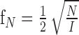
In Figure 2, we plot the measured spatial stereoresolution as a function of dot density. The filled diamonds represent stereoresolution thresholds measured at the short viewing distance with a disparity modulation of 16 min arc. The diagonal line is the Nyquist frequency (Eq. 1). Data from another two observers are presented in the supplementary on-line material (Fig. S1).

Figure 2.

Spatial stereoresolution as a function of dot density. The highest discriminable corrugation frequency is plotted as a function of the dot density of the stereogram. Each panel shows results from one observer (JMA in the top panel and MSB in the bottom panel). Results from two more observers are shown in Figure S1 in the supplementary on-line material. The filled diamonds represent the measured resolution when the disparity amplitude was 16 min arc, and the open squares represent the resolution when the amplitude was 4.8 min arc. The solid lines represent the Nyquist sampling limit f_N of the dot pattern (Eq. 1). Viewing distance was 39 cm. The error bars are ±1 SD.

For a nearly 2-log-unit range of dot density [0.15-10 dots/deg² (i.e., all but the highest dot densities)], the data have a slope of 0.5 in log-log coordinates. This means that performance is scale invariant for nearly the entire range of densities. An implication of scale invariance is that a stimulus that is just discriminable at one corrugation frequency and dot density will also be just discriminable when viewed across a wide range of distances. (Note that this is not strictly correct. A change of viewing distance changes the disparity amplitude in addition to the corrugation frequency and dot density.)

The observers' phenomenology suggests that they were reconstructing substantial portions of the disparity waveform. That is, they were unable to judge its orientation unless they perceived a portion of the corrugated surface. If an observer attempts to reconstruct the depth surface z = f(x,y) from the perfectly measured sample disparities, then Equation 1 applies, assuming the surfaces are drawn from the set of low-pass depth functions with cutoff frequency f_N. The data in the scale-invariant range in Figure 2 are close to the Nyquist frequency, which is consistent with this idea. (For additional discussion of the number of samples required to perform the psychophysical task, see supplementary on-line material, Number of Required Samples for Ideal Discriminator.)

How many samples were required to identify the disparity waveform reliably for the part of the data that follow the Nyquist limit? Consider a cross-section orthogonal to the disparity waveform (i.e., in the direction of greatest disparity variation). In this direction, the Nyquist rate calls for two samples per stimulus cycle. Thus, for a square patch, whose width and height are equal to one stimulus cycle, observers required four dots on average to perform the task reliably.

Independence of sample placement

The preceding discussion did not mention the locations of the sample points. In principle, it hardly matters where the sample points are located, as long as they are reasonably well positioned. One way to understand this is to count degrees of freedom: each sample point provides a single measurement of disparity; as long as there are as many such measurements as there are independent values in the low-pass Fourier transform of the depth function, the function can be reconstructed successfully. One effect of sample location is that the stability of reconstruction worsens with increasing deviation from a regular sampling grid (Maloney, 1996). The size and shape of the dots themselves have no effect on the ability to reconstruct the waveform as long as the centers represent the disparity at that point and the reconstruction algorithm uses the center positions.

Although dot positioning and dot size may not matter for surface reconstruction (assuming perfect dot correspondences), it may well have an effect on the observer's ability to determine correspondences, because those parameters alter the luminance spatial-frequency content of the images (see Does low-pass spatial filtering limit spatial stereoresolution?). Three types of random-element stereograms have been used in the literature. First, there is the random-dot stereogram introduced by Julesz (1960) and then used by Rogers and colleagues (Rogers and Graham, 1982, 1983; Bradshaw and Rogers, 1999) to investigate the spatial resolution of stereopsis. This stimulus is a grid of randomly colored squares, one-half black and one-half white. For Julesz, disparities are limited to integer multiples of the discrete grid; for Rogers, disparities finer than the grid were presented. Second, there is the sparse random-dot stereogram in which dots are placed in random positions, and anti-aliasing techniques allow the presented disparity increments to be far smaller than the dot size (Tyler, 1974; Lankheet and Lennie, 1996; Nienborg et al., 2004). Third, in our study, we used sparse dots, but the positions were based on a jittered hexagonal lattice to avoid the formation of clumps of dots (clumps are regions in which the dot density is much higher than in other regions).

Does the type of stereogram affect stereoresolution? The top row of Figure 3 displays examples of the monocular images created by two types of stereograms. The top left panel is one of the monocular images created by our jittered-lattice technique. Its luminance amplitude spectrum is displayed in the inset. The spectrum contains components with orientations at every 60° with a corrugation frequency of 1/s, where s is the spacing between the elements of the original unperturbed lattice. The top right panel displays a monocular image from a sparse random-dot stereogram (Nienborg et al., 2004). It has no periodicity, so the spectrum is flat up to a cutoff determined by the dot size. (The cutoff is farther from the origin than the boundaries of the inset, because the stimulus dots are small.)

Figure 3.

Jittered-lattice and sparse random-dot stereograms. Top row, Half images associated with the two types of stereograms. Bottom row, Spatial stereoresolution as a function of dot density for the two types of stereograms. Top left, The larger image is a monocular image from a jittered-lattice stereogram such as the ones used in the current study. See Materials and Methods for details. The inset is the amplitude spectrum of this monocular image. Top right, The larger image is a monocular image from a sparse random-dot stereogram such as the ones used by Nienborg et al. (2004). The inset is the amplitude spectrum of this monocular image. The two bottom panels plot the highest discriminable corrugation frequency as a function of dot density. Each panel shows results from one observer (MSB and SSG). The open squares represent resolution for a jittered-lattice stereogram (Fig. 1 and top left panel), and filled circles represent resolution for a sparse random-dot stereogram (top right panel). Disparity amplitude was 4.8 min arc, viewing distance was 39 cm, and stimulus duration was 600 msec. The solid lines represent the Nyquist sampling limit f_N of the dot pattern (Eq. 1). The error bars are ±1 SD.

For a given dot density, the jittered-lattice and sparse random-dot stereograms should in principle support the same spatial resolution for stereopsis, despite the clear differences in their luminance spectra. We tested this by measuring stereoresolution in two observers with the jittered-lattice (see Materials and Methods) and sparse random-dot stimuli. The sparse random-dot stereograms were generated from a uniform random distribution of two-dimensional dot positions before applying the disparity as specified in Equation 2. For both types of stereogram, disparity amplitude was 4.8 min arc, viewing distance was 39 cm, and stimulus duration was 600 msec.

The results are shown in the bottom row of Figure 3, which plots spatial stereoresolution as a function of dot density for the two types of stereogram. The data are clearly very similar for the two types of stimuli, which means that the technique for distributing the dots does not affect resolution. In both cases, the data are quite close to the Nyquist frequency at all but the highest dot densities. The similarity of the results allows us to compare our psychophysical data with the physiological findings of Nienborg et al. (2004).

Effect of disparity gradient

In the first experiment, stereoresolution leveled off at 1-2 cycles/° for dot densities >10 dots/deg² (Fig. 2, filled diamonds). What caused this asymptote? That is, why did the measured resolution not continue to rise as predicted by the Nyquist limit at the higher dot densities?

The disparity gradient of the stimulus may well limit performance. A pair of horizontally separated points forms angles α_L and α_R at the left and right eyes, respectively. The disparity is the difference in the angles: δ = α_R - α_L. The angular separation is the average of the angles: x = (α_L + α_R)/2. The disparity gradient is the ratio: δ/x = 2(α_R - α_L)/(α_L + α_R). The disparity gradient is zero for points with zero disparity (points on the horopter) and infinite for points aligned in depth (points with zero angular separation). When the disparity gradient is ∼1 or higher, binocular fusion breaks down. The gradient at which this occurs has been called the disparity gradient limit (Burt and Julesz, 1980). It is important to note that the disparity gradient created by a planar surface is affected by surface slant (larger gradients for larger slants) and by viewing distance (smaller gradients for a given slant with increasing distance).

As corrugation frequency increases, the stimulus can exceed the disparity gradient limit, and this could cause a failure in disparity measurement (Ziegler et al., 2000). The disparity gradient varies across a sinusoidal disparity waveform, but is proportional to corrugation frequency. For example, the gradient between the peaks and troughs is 2Af, where A is peak-to-trough amplitude and f is corrugation frequency.

If approaching or exceeding the disparity gradient limit caused the asymptote in the data in Figure 2 (filled diamonds), then reducing the disparity amplitude should yield higher resolution at high dot densities. To test this, we next measured spatial stereoresolution with the disparity amplitude reduced from 16 to 4.8 min arc (Fig. 2, open squares). Resolution improved at high dot densities. Thus, the disparity gradient limit constrained resolution in the first experiment.

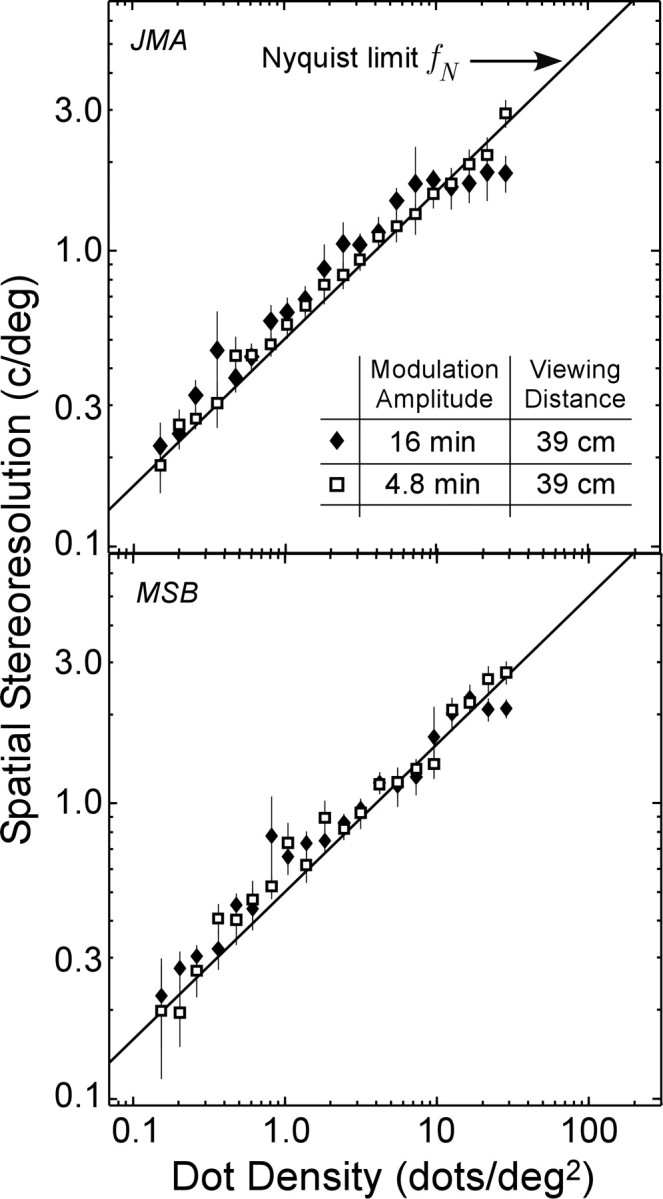
Resolution limit independent of constraints attributable to sampling and disparity gradient

If stereoresolution were constrained only by the Nyquist limit and the disparity gradient limit, there would be no limit to the highest measurable resolution at sufficiently high dot densities and sufficiently low disparity amplitudes. However, previous investigators have argued that spatial stereoresolution reaches a limiting value that is independent of dot density and disparity amplitude (Tyler, 1974; Bradshaw and Rogers, 1999). One could determine whether such a limit exists by testing at higher dot densities, but monocular artifacts intrude at high densities as luminance variations correlated with stimulus orientation become visible. Thus, to make measurements at higher dot densities, we had to reduce the retinal-image size of the dots. We did so by increasing viewing distance from 39 to 154 cm. Disparity amplitude was again 4.8 min arc. We also minimized blur in the retinal images by placing appropriate spherical and cylindrical ophthalmic lenses before the observers' eyes. We confirmed that monocular artifacts did not contribute to performance by conducting a monocular control experiment (see supplementary on-line material). By determining the combinations of corrugation frequency and dot density that created artifacts, we avoided using those stimuli in the binocular experiment. Stimulus duration was increased to 1500 msec, because observers had to cross-fuse in the experimental setup for the longer viewing distance, and they found this difficult at short durations.

The filled circles in Figure 4 represent the measured resolution at the long viewing distance (the open squares are the low-amplitude data from the short viewing distance, reported previously in Fig. 2). At low dot densities, resolution is again close to the Nyquist limit. At high densities, however, resolution reaches 2-4 cycles/° before leveling off. The asymptote (departure from the diagonal line) cannot be explained by the sampling properties of the stimulus. Data from two additional observers are shown in Figure S2 of the supplementary on-line material.

Figure 4.

Spatial stereoresolution as a function of dot density at two viewing distances (two observers, JMA and MSB). The open squares represent the measured resolution at a viewing distance of 39 cm, and the filled circles represent the resolution at a distance of 154 cm. The solid lines again represent the Nyquist sampling limit (Eq. 1). Disparity amplitude was 4.8 min arc. Results from two more observers are shown in Figure S2 in the supplementary on-line material. The error bars are ±1 SD.

Perhaps the disparity gradient limit caused the asymptote in the data in Figure 4. We tested this idea in two ways. First, we asked what the asymptote would have been in the second experiment (Fig. 4) if the disparity gradient were the only limit to asymptotic performance. If it were the only limit, asymptotic resolution would be proportional to disparity amplitude. Because the ratio of amplitudes was 3.3 [16 min arc in Fig. 2 (filled diamonds) and 4.8 min arc in Fig. 4 (filled circles)], the ratio of asymptotic acuities should also be 3.3. Thus, if disparity gradient were the only limit to stereoresolution at high dot densities, the highest resolution in the second experiment (Fig. 4) would have been ∼6 cycles/°. The asymptotic resolution is clearly lower than this, which implies that lowering the disparity amplitude further would not have yielded an improvement in resolution. Second, we confirmed this by making a few measurements at a lower disparity amplitude of 2.4 min arc. We found no improvement in resolution.

In conclusion, there is apparently a limit to the highest measurable spatial stereoresolution beyond those specified by the Nyquist limit and the disparity gradient limit. Our main goal in the remainder of the paper is to reveal the determinants of the highest measurable spatial stereoresolution.

Does low-pass spatial filtering limit spatial stereoresolution?

Low-pass spatial filtering (attenuation of high spatial frequencies relative to low and intermediate frequencies) at the front end of the visual system limits performance in many tasks including luminance contrast sensitivity (Banks et al., 1987, 1991; MacLeod et al., 1992; Chen et al., 1993), visual acuity (Levi and Klein, 1985), and motion sensitivity (McKee and Nakayama, 1984). The physiological mechanisms that contribute to the low-pass filtering include the optics of the eye, receptor optics, and pooling of receptors in the construction of higher-order receptive fields. We examined the contribution of low-pass spatial filtering to spatial stereoresolution in two ways: (1) we blurred the stimuli to examine how low-pass filtering of the stimulus affects the measured resolution, and (2) we made measurements at various retinal eccentricities to examine how low-pass filtering in the visual system affects resolution.

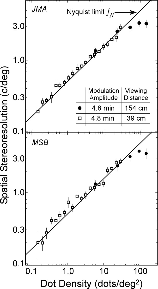
To vary stimulus blur, we placed diffusing screens in front of the monitors. The stimuli were otherwise identical with those in the second experiment (Fig. 4). There were three levels of blur: none, low, and high. We determined the point spread functions of the diffusing screen at the two distances from measurements of an observer's luminance contrast sensitivity. Three contrast sensitivity functions were measured: with no screen, with the screen at the near distance, and with the screen at the far distance. The ratio of contrast sensitivities (screen-in-place divided by no-screen) gives the modulation transfer function associated with the diffusion screen at the eye. Inverse Fourier transformation then yields the point spread function. Those point spread functions for the low- and high-blur levels at the viewing distance of 154 cm were well described by two-dimensional Gaussians with SDs of 0.05 and 0.10°.

The results of the blur experiment are shown in Figure 5. Stereoresolution followed the Nyquist limit at low dot densities and leveled off at higher densities. The spatial frequencies at which resolution leveled off depended on the amount of blur: 4-5 cycles/° with no blur, 1-2 cycles/° with low blur, and 0.7-1 cycle/° with high blur. Thus, stereoresolution is limited by the sampling properties of the stimulus at low dot densities and by its luminance spatial-frequency content at high densities.

Figure 5.

Spatial stereoresolution as a function of dot density with different amounts of stimulus blur (two observers, JMA and MSB). The filled circles represent the measured resolution with no blur, the filled triangles represent the resolution at the low-blur level, and open squares represent the resolution at the high-blur level at the viewing distance of 154 cm. The solid lines again represent the Nyquist limit. Disparity amplitude was 4.8 min arc. The error bars are ±1 SD.

We also varied the retinal eccentricity of the stimulus to determine how variations in low-pass filtering within the visual system affect stereoresolution. The stimuli were the same as those of the first experiment (Fig. 2) except that the disparity modulation was restricted to an elliptical patch. To avoid edge artifacts, the modulated region had Gaussian skirts (SDs of 6.25° horizontally and 5° vertically) surrounding an elliptical region (6.25 × 5°) of uniform disparity modulation. The patches were presented at three positions relative to the fixation point: at fixation and at two positions below fixation. The values of the two nonfoveal eccentricities differed for the two observers: the largest eccentricity was set to produce just-visible disparity modulation for each observer, and the intermediate eccentricity was one-half the value of the largest one. Observers maintained fixation throughout testing. Viewing distance was 39 cm, stimulus duration was 250 msec, and disparity amplitude was 16 min arc. By using the shorter duration and by interleaving eccentricities randomly in a given experimental session, we minimized the probability of eye movements toward the stimulus patch. The larger disparity amplitude was required for observers to do the task in the periphery. The resolution values were low, so the disparity gradient limit did not constrain performance in the peripheral measurements.

The results for two observers are shown in Figure 6; results for another observer are provided in Figure S3 of the supplementary on-line material. At each retinal eccentricity, we again observed a clear effect of dot density: with increasing density, the measured resolution increased (following the Nyquist limit) up to a point after which it leveled off. The resolution reached an asymptote at quite different values: nearly 2 cycles/° at the fovea, ∼1 cycle/° at the intermediate eccentricity, and ∼0.3 cycle/° at the largest eccentricity tested (Prince and Rogers, 1998). Could the decline in resolution with retinal eccentricity be caused by an overall deficit in binocular processing in peripheral vision? The data at low dot densities suggest otherwise, because at those densities, the measured resolution was essentially the same at all of the eccentricities (and followed the Nyquist limit). In other words, resolution decreased only at high dot densities at which, as we showed in the blur experiment, performance is limited by the luminance spatial-frequency content of the stimulus. Spatial filtering at the front end of the visual system has a successively lower frequency cutoff with increasing retinal eccentricity (Banks et al., 1991) and almost certainly occurs before the first site of binocular interaction (Chen et al., 1993). The cause of the eccentricity-dependent reduction in cutoff frequency in the luminance domain is a combination of low-frequency filtering attributable to poorer optics and larger photoreceptors and of larger receptive fields (Banks et al., 1991). For similar reasons, the findings in Figures 5 and 6 suggest that the variation in spatial stereoresolution with retinal eccentricity is not attributable to a binocular deficit in the periphery, but rather to low-pass spatial filtering attributable to the optics and the use of larger receptive fields before binocular interaction.

Figure 6.

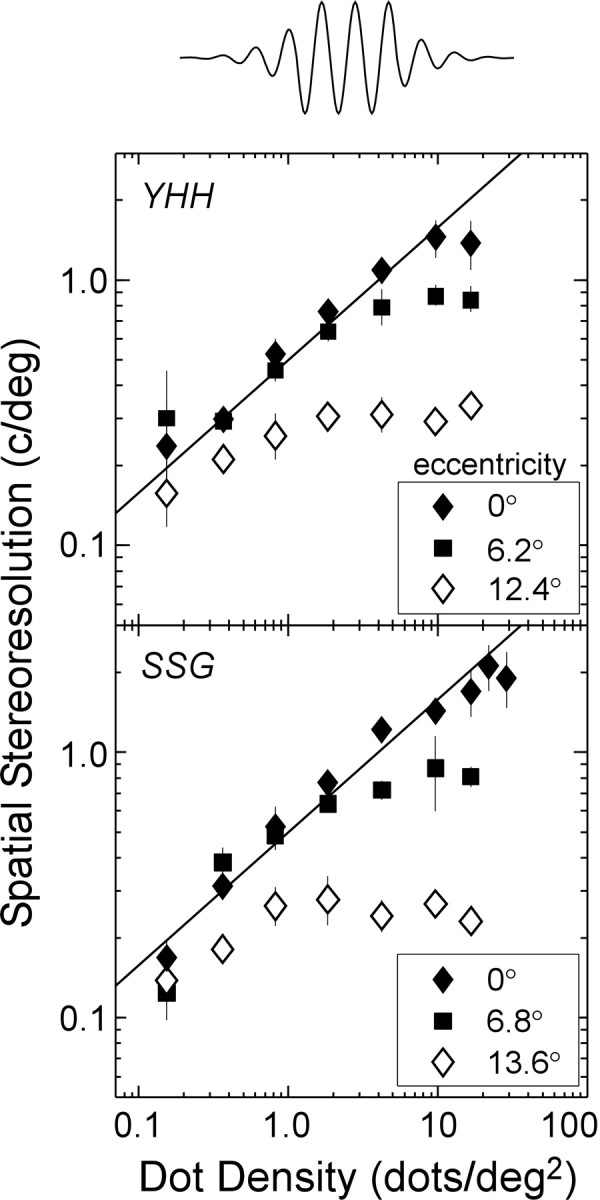
Spatial stereoresolution as a function of dot density at different retinal eccentricities (two observers, YHH and SSG). The stimuli were a full field of random dots with a small region in which the disparity modulation was present. A cross-section of the disparity modulation is shown at the top. The filled diamonds represent the measured resolution at fixation (eccentricity, 0°), the filled squares represent the resolution at the intermediate eccentricity, and the open diamonds represent the resolution at the large eccentricity. The solid lines again represent the Nyquist limit. Disparity amplitude was 16 min arc, viewing distance was 39 cm, and stimulus duration was 250 msec. Results from one more observer are shown in Figure S3 in the supplementary on-line material. The error bars are ±1 SD.

Does the process of binocular matching determine spatial stereoresolution?

Random-dot stereograms have the virtue of minimizing or eliminating nonbinocular cues to depth, but have the drawback of making binocular matching difficult. In regard to the matching problem, the dots in such stereograms generally do not differ in size, shape, or luminance, so information from the dots themselves does not restrict the possible matches between the two retinal images. The problem for the visual system is to distinguish the correct from incorrect matches. We next asked whether limitations resulting from the binocular-matching process caused stereoresolution to level off at 2-4 cycles/° (Figs. 2 and 4). We tested this possibility by examining computationally the properties of a binocular-matching algorithm based on cross-correlation of the two retinal images.

Description of the algorithm

Binocular matching by computing correlation is a basic and well studied technique for obtaining a depth map from binocular images. Several computational studies have examined matching by correlation (Tyler and Julesz, 1978; Jenkin and Jepson, 1988; Cormack et al., 1991; Kanade and Okutomi, 1994; Weinshall and Malik, 1995). Furthermore, the properties of binocular neurons in the striate cortex suggest that the estimation of disparity begins with signals closely related to binocular correlation measured after the image is filtered by monocular receptive fields (Ferster, 1981; Qian and Zhu, 1997; Anzai et al., 1999). Indeed, Fleet et al. (1996) (their Eqs. 20 and 21) and Anzai et al. (1999) (their Eqs. 5-8) pointed out the mathematical equivalence between interocular correlation and the disparity energy calculation that underlies binocular interaction in V1 neurons (Ohzawa et al., 1990; Cumming and Parker, 1997). The accompanying paper (Nienborg et al., 2004) suggests that the size of V1 receptive fields limits the ability of single neurons to detect spatial variation in disparity. We therefore examined whether an algorithm based on correlation might explain our results. With this technique, the size of the correlation window must be large enough to include sufficient luminance variation. If the window is not large enough, the disparity estimate will be poor because the signal (luminance variation)-to-noise ratio is low. In contrast, if the image region of interest contains significant depth variation, the window cannot be too large, because the correlation algorithm will yield an estimate close to the average disparity and will therefore fail to detect the disparity variation. Kanade and Okutomi (1994) developed a binocular-matching algorithm that searches for the optimal window size and shape. Specifically, the iterative algorithm finds the window size and shape for each location in the image that yields the disparity estimate of least uncertainty. In image regions with significant depth variation, small windows yield the best disparity estimate and in image regions with little depth variation, large windows yield the best estimate.

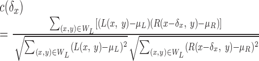
The insight that the best correlation window size depends on the depth variation in the image is directly relevant to the issues under examination here. To explore the relationship between spatial stereoresolution and the size of the correlation window, we constructed a correlation algorithm for estimating disparity. The inputs to the algorithm were bitmaps from the stimuli used in our experiment. The bitmaps were convolved with the point spread function of the well focused eye (Campbell and Gubisch, 1966) (3.8 mm pupil). Poisson noise (variance proportional to intensity) was then added to each point. The resulting images were input to the binocular-matching algorithm, the main features of which are depicted in Figure 7. A square correlation window W_L was placed in the left eye image (the thick square); its width and height were w. That window was moved on a line (oblique arrow) through the middle of the image and orthogonal to disparity corrugation. For each position of the left eye window, a square window W_R was placed in the right image (the thin square); its width and height were also w. We capitalized on the epipolar constraint (Howard and Rogers, 2002) and restricted the movement of the window of the right eye to a horizontal line (horizontal arrow) through the midpoint of the left eye window. For each position of the window of the left eye, we computed the cross-correlation between the two windowed images:

3

Figure 7.

Schematic of the correlation algorithm for binocular matching. The left and middle panels are the images presented to the left and right eye. The corrugation waveform is oriented 20° counterclockwise from horizontal. A square correlation window was placed in the image of the left eye (thick square); its width and height were w. That window was moved on a line (oblique arrow) through the middle of the image and in a direction orthogonal to disparity corrugation. For each position of the left eye window, a square window was placed in the right eye image (thin square); its width and height were also w. We restricted the movement of the window of the right eye to a horizontal line (horizontal arrow) through the midpoint of the window of the left eye. For each position of the window of the left eye, we computed the cross-correlation between the two windowed images (Eq. 3). The right panel shows the output of the algorithm. The abscissa is the position of the window in the left eye image (along the oblique arrow), and the ordinate is the relative position of the window in the right eye image (along the horizontal arrow) (i.e., horizontal disparity). For ease of viewing, the scale of the ordinate has been magnified relative to the scale of the abscissa. Correlation is represented by intensity, brighter values corresponding to higher correlations. In this particular case, the algorithm produced a sinusoidal ridge of high correlation corresponding to the sinusoidal disparity signal.

The image intensities were L(x,y) and R(x,y) for the left and right eyes, and the mean intensity within each window was μ_L and μ_R. The cross-correlation c was computed for all of the horizontal shifts δ_x of the right eye image relative to the left eye image.

An example of the output is displayed in the right panel of Figure 7. The x-axis represents the position of the window in the left image (orthogonal to the corrugations), and the y-axis represents the horizontal position of the window in the right eye image relative to the left eye image (i.e., the horizontal disparity, δ_x). Correlation is represented by the gray-scale value, higher correlations by higher intensities. There is a ridge of high correlation corresponding to the sinusoidal disparity waveform, so in this case the algorithm detected the signal. It would be useful to have a quantitative decision rule, such as an ideal discriminator, that used the output of the correlation algorithm to make a psychophysical decision. However, the development of such an ideal discriminator is beyond the scope of this paper, so we will study the correlation algorithm by examining its output for a variety of situations.

Effect of window size

There are two general cases in which the output of the algorithm does not provide a clear signal: when the correlation window is too small and when it is too large. Figures 8 and 9 exemplify those two situations.

Figure 8.

Effect of window size and dot density on binocular matching by interocular correlation. Each panel displays the correlation as a function of position of the window in the left and right eyes. The scale of the ordinate has been magnified relative to the scale of the abscissa. The inset represents the spatial frequencies and dot densities for the stimuli that were used to generate the outputs shown in the four panels. A and C show outputs for the same stimulus: corrugation frequency, 0.32 cycle/°; dot density, 0.74 dots/deg². B and D show outputs for a stimulus with a higher dot density of 6.6 dots/deg². A and B have a correlation window of 0.22 × 0.22°, and C and D have a window of 0.66 × 0.66°.

Figure 9.

Effect of window size and corrugation frequency on binocular matching by interocular correlation. The scale of the ordinate has been magnified relative to the scale of the abscissa. The inset represents the spatial frequencies and dot densities for the stimuli that were used to generate the outputs shown in the four panels. A and B show outputs for the same stimulus: corrugation frequency, 1.3 cycles/°; dot density = 18.5 dots/deg². C and D show outputs for a stimulus with a lower corrugation frequency of 0.32 cycle/°. A and C have a correlation window of 0.66 × 0.66°, and B and D have a window of 0.22 × 0.22°.

Figure 8 shows how the best window size for disparity estimation depends on the density of samples in the stimulus. The outputs of the algorithm are shown for combinations of two dot densities—0.74 and 6.6 dots/deg² (left and right columns, respectively)—and two window sizes—0.22 × 0.22° and 0.66 × 0.66° (top and bottom rows). In Figure 8D, the stimulus has relatively high dot density and the correlation window is large; the output reveals a correlation surface that signals the disparity waveform clearly. Figure 8B shows the output for the same stimulus, but with a much smaller correlation window. Disparity estimation is worse, because fewer samples are available within the correlation window. Figure 8, A and C, shows the output of the algorithm for the small and large correlation windows, respectively, when dot density is relatively low. In both cases, disparity estimation is poor, because there is an insufficient number of samples within the correlation window. Thus, Figure 8 illustrates that failures in disparity estimation occur whenever there are too few samples in the correlation window. We found that disparity estimation suffers whenever the correlation window contains on average slightly less than 1 dot. The critical number of samples per correlation window also depends on the luminance spatial-frequency content of the monocular images (see Effect of low-pass spatial filtering).

Figure 9 shows how the best window size for disparity estimation depends on the spatial frequency of the disparity waveform. The outputs of the algorithm are shown for combinations of two frequencies—1.3 and 0.32 cycles/° (top and bottom rows, respectively)—and two window sizes—0.66 × 0.66° and 0.22 × 0.22° (left and right columns). The output in Figure 9C shows that disparity estimation is excellent for the lower corrugation frequency and larger window. In Figure 9D, the area of the correlation window has been reduced, and again disparity estimation is excellent. Now we increase the corrugation frequency of the disparity waveform. In Figure 9A, disparity estimation is poor, because the window is large relative to the period of the corrugation: the estimate is like a thickened frontoparallel plane rather than the sinusoidal waveform. The estimate is much better in Figure 9B, because the window is small relative to the period of the corrugations. Thus, shrinking the correlation window can significantly improve disparity estimation when dot density and corrugation frequency are high. We found that disparity estimation suffers significantly whenever the width of the correlation window is >50% of the spatial period of the disparity waveform.

We can summarize the behavior of the correlation algorithm by plotting, in the format of the data figures, the corrugation frequency at which disparity estimation begins to fail. For each window size, there is a corrugation frequency above which performance levels off; as we said, this occurs whenever the period of the disparity waveform becomes small relative to the size of the correlation window. The asymptotic resolution value is, therefore, inversely proportional to window width:

4

The top edges of the three shaded areas of Figure 10 represent those critical frequencies for correlation windows of 0.22 × 0.22°, 0.66 × 0.66°, and 1.98 × 1.98°. For each window size, there is also a dot density below which the algorithm fails; as we said, this occurs whenever the number of dots falling within the correlation window on average is ∼1 (meaning that many image regions allow >1 dot per window). Therefore, the limiting dot density is inversely proportional to window area:

5

Figure 10.

Critical spatial frequencies and dot densities for different window sizes. The correlation algorithm exhibits an asymptotic resolution a, which is inversely proportional to window width w. The top edges of the tall, intermediate, and short shaded areas represent that asymptotic frequency for correlation window sizes of 0.22 × 0.22°, 0.66 × 0.66°, and 1.98 × 1.98°, respectively. The correlation algorithm also exhibits a limiting dot density d that is inversely proportional to window area. The left edges of the tall, intermediate, and short shaded areas represent that critical density for correlation windows of 0.22 × 0.22°, 0.66 × 0.66°, and 1.98 × 1.98°, respectively. The diagonal line is a plot of Equation 6, which has a slope of 0.5 in this log-log plot. The shaded areas represent the combinations of corrugation frequency and dot density for which each of the three correlation windows would estimate disparity accurately.

The left edges of the shaded areas represent those critical densities for the three window sizes. The shaded areas represent the combinations of corrugation frequency and dot density that yield good disparity estimation for each of the three correlation windows.

For each combination of dot density and corrugation frequency, there is an optimal size for the correlation window. If we measured the stereoresolution of the algorithm as a function of density, and the optimal window was always used, the resolution would trace out a line of slope 0.5 (the corners of the shaded areas shows those resolution values for three window sizes). The positions of the corners can be found approximately by substituting for w in Equation 4 and taking the logarithm:

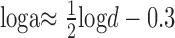6

The oblique line in Figure 10 represents Equation 6. As suggested by the line, the highest resolution would be achieved with the smallest available window, provided that the window contained a sufficient signal (luminance variation)-to-noise ratio. Note that the slope is unaffected by the choice of constants in Equations 4 and 5. The stereoresolution we measured experimentally also traced out a line of slope 0.5 (Fig. 2) at all but the highest densities, so binocular matching based on correlation with adaptive window sizes yields a scale-invariant dependence between dot density and spatial stereoresolution like the one we observed psychophysically.

Effect of window shape

For straight depth edges in the scene, Kanade and Okutomi (1994) found that rectangular windows elongated parallel to the edge yielded the best disparity estimates. With sinusoidal disparity waveforms, the maximum disparity gradient has a constant direction (orthogonal to the corrugations), so a window with width w in the direction of the gradient but length much greater than w in the orthogonal direction would contain more intensity variation than a square window of width and height w. For this reason, an elongated window would provide a better disparity estimate without blurring the signal at high spatial frequencies (as occurred in Fig. 9A) and would thereby enable higher resolution. We did not include elongated windows in our modeling, because disparity-selective V1 neurons, which we believe are the biological analog of the interocular cross-correlator, typically do not have greatly elongated receptive fields.

Effect of disparity gradient

Recent models describe binocular matching in terms of spatial filtering (Ohzawa et al., 1990; Fleet et al., 1996; Cumming and Parker, 1997; Qian and Zhu, 1997; Anzai et al., 1999), so in that framework, solving the matching problem is tantamount to finding similar filter outputs from the two eyes. For the outputs of matched filters to be similar, their inputs must be similar, so binocular matching in this scheme requires similar local intensity patterns in the left and right retinal images. The local patterns in the two eyes are quite different when the disparity gradient is high, because a large gradient in part of the binocular stimulus means that the one image is stretched or sheared horizontally relative to the other. In the accompanying paper, Nienborg et al. (2004) show that disparity-selective V1 neurons respond best when the disparity gradient is near zero.

We examined the influence of the disparity gradient by examining the behavior of the correlation algorithm for different disparity amplitudes. Figure 11 shows the results. From left to right, amplitudes were 4.8, 13.6, and 40.8 min arc. The corresponding peak-to-trough disparity gradients were 0.21, 0.59, and 1.77. Notice that disparity estimation became progressively poorer as the amplitude (and gradient) was increased. This suggests that the disparity gradient limit (Burt and Julesz, 1980) is caused by the difficulty of matching by correlation when the gradient is large. We also examined the effect of the direction of the disparity gradient (i.e., vertical for horizontal corrugations, horizontal for vertical corrugations) and found no obvious differences in the gradient magnitude at which estimation broke down. This is consistent with the psychophysical observation that the disparity gradient limit is constant across directions (that is, constant across tilts) (Burt and Julesz, 1980).

Figure 11.

Effect of disparity gradient on binocular matching by interocular correlation. The corrugation frequency and dot density of the stimuli are the same for each panel (f = 1.3 cycles/°; d = 18.5 dots/deg²), and the size of the correlation window is the same (w = 0.22°). The disparity amplitude increases nearly ninefold from the left panel to the right: amplitude, 4.8 min arc (A), 13.6 min arc (B), and 40.8 min arc (C).

It is interesting to note that the correlation algorithm finds the highest correlations in the peaks and troughs of the disparity waveform where the disparity gradient becomes zero. This is particularly evident in Figure 9B. The algorithm finds the highest correlations in the parts of the stimulus that are frontoparallel [strictly speaking, in the parts that are tangent to the Vieth-Müller circle (see Spatial stereoresolution and binocular matching in area V1)].

Effect of low-pass spatial filtering

We next examined the effect of spatial filtering before computing the correlation between the two retinal images. Let L(x,y) and R(x,y) represent image intensities in the left and right eyes. Let s(x,y) represent all of the linear spatial filtering before interocular correlation, including the point spread function of the dots themselves, blurring attributable to the diffusion screens (Fig. 5), and the optical point-spread function of the eye. Thus, the filtered images delivered to the correlation algorithm are:

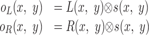7

where ⊗ represents convolution. (It is interesting to note that because convolution is commutative, one can equivalently apply the spatial filtering before the cross-correlation to the eyes' images separately or apply the filtering twice after cross-correlation.)

As shown previously, when the correlation window is too small, disparity estimation is poor, because the window does not cover enough intensity variation (Fig. 8A) (Kanade and Okutomi, 1994). Naturally, the amount of intensity variation in a region of the image is highly dependent on the luminance spatial-frequency content of the image. Figure 12 illustrates the relationship between spatial filtering, window size, and regional intensity variation. [Hess et al. (1999) described a similar relationship between luminance frequency content and disparity modulation sensitivity.] Each of the five insets represents a monocular image captured by a correlation window. Dot density in the insets ranges from 1 to 100 dots/deg² from left to right. The width of the correlation window is , which is large enough to include on average approximately six samples per window. If σ, the space constant that represents blur, is proportional to w (which, in turn, is inversely proportional to ), then the intensity variation expressed in cycles per window is constant (apart from random variation attributable to the nature of the jittered lattice and Poisson noise). Figure 12 illustrates this invariance: the insets all have the same variation in cycles per window. If dot density is high and proportional to 1/w² (Eq. 5), and the spatial frequency of the disparity corrugation is proportional to 1/w (Eq. 4), we find that the correlation algorithm yields similar outputs for all of the images that follow the scale invariance line in the figure. Thus, for each σ, there is a window size that is just large enough to yield reasonable disparity estimates (w ∝ σ), and consequently, the highest detectable corrugation frequency is inversely proportional to σ.

Figure 12.

Effect of low-pass spatial filtering and scale invariance of spatial stereoresolution. The five insets represent a monocular image as seen by a correlation window. Dot density in the inset images ranges from 1 to 100 dots/deg² from left to right. The width of the correlation window is inversely proportional to dot density: , large enough to include on average approximately six samples per window. The low-pass spatial filter is represented by an isotropic Gaussian. The SD σ of the Gaussian is proportional to w: σ = w/2.5. The intensity variation expressed in cycles per window is constant across the insets (apart from random variation in the stimulus) because of the proportionalities between the dot density d, window size w, and blur constant σ. The diagonal line represents the Nyquist limit. Our data suggest that stereoresolution expressed in cycles per degree would fall along a positive diagonal for these stimuli, so we placed the insets on a diagonal of the same slope as the Nyquist limit, but below the limit.

An important question is whether the space constant of the spatial filter, when applied to the correlation algorithm, predicts the resolution at which performance leveled off in the main experiment (Fig. 4), in the blur experiment (Fig. 5), and in the retinal-eccentricity experiment (Fig. 6). Unfortunately, to answer this quantitative question rigorously, one has to develop an information-preserving decision rule (an ideal discriminator) and then apply it to the output of the algorithm. With such a decision rule, we could obtain quantitative predictions and compare them with human data. The development of an ideal discriminator is beyond the scope of this paper, but the scale-invariant property of the algorithm allows us to predict the ratios of resolutions as σ is varied. Specifically,

8

where a is the resolution, and the subscripts refer to different conditions. Figure 13 shows the data from Figure 5. The filled circles, filled triangles, and open squares represent the measured resolution for the no-blur, low-blur, and high-blur conditions, respectively. The σ_c values in the figure represent the space constants when all of the filtering elements—the dots themselves, the optics of the eye, and the diffusion screen—are taken into account. The σ_c values were substituted in Equation 8 to generate predictions for the ratios of resolutions. We fit the horizontal lines by eye to the asymptotic resolution values in the high-blur condition (open squares), and then used the ratio predictions from Equation 8 to position the lines for the low-blur and no-blur conditions. The predictions are reasonably good, which raises the possibility that the fundamental limit to the asymptotic resolution is low-pass filtering of the stimulus before it reaches the site of interocular combination.

Figure 13.

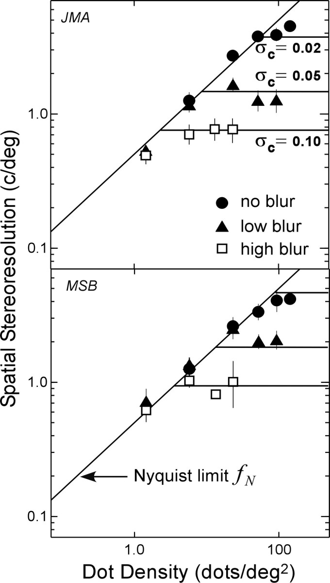
Observed and predicted stereoresolution as a function of blur. The data points are the same as the ones in Figure 5 (two observers, JMA and MSB). Filled circles represent resolution when no external blur was added to the stimulus. Filled triangles represent resolution when we added external blur with a space constant of 0.05° by placing a diffusion screen in front of the display. Open squares represent resolution when we added external blur with a space constant of 0.10°. The space constants that incorporate all of the components of spatial filtering—the dots themselves, the diffusion screen, and the point spread function of the eye—were calculated from the sums of the squared space constants of the components. Those constants σ_c were 0.02, 0.05, and 0.10° for the no-blur, low-blur, and high-blur conditions, respectively. The low- and high-blurσ_c values (the space constants for all of the blur elements) are similar to the σ values for the diffusion screen alone, because the screen caused much greater blur than the optics of the eye and the spread of the dots themselves on the CRT. The lowest of the horizontal lines was fit to the asymptote in the high-blur condition. Then we used Equation 8 to predict the ratios of resolution values from the ratios of space constants. The other two horizontal lines in each panel represent the predictions.

If this speculation is correct, spatial filtering occurring before the site of binocular interaction could determine the highest attainable spatial stereoresolution. In turn, the prebinocular filter determines the smallest useful receptive field for computing binocular correlation (Nienborg et al., 2004). Still, observers might use windows larger than the smallest available receptive field. We cannot tell from our data whether that is the case. To do so would require a model of how the correlation outputs are used to make the psychophysical judgment. Finally, we should point out that blur caused by spatial filtering might have a different quantitative effect on stereoresolution measured with line stereograms (Tyler, 1973) as opposed to the random-element stereograms considered here.

Discussion

We began by asking why spatial stereoresolution is so low compared with similar tasks in the luminance domain. We examined the contributions of three stimulus factors: (1) sampling limitations imposed by the discrete nature of the random-element stereogram, (2) the disparity gradient limit, and (3) low-pass spatial filtering before binocular combination. We found that all three limit stereoresolution. Our main findings are illustrated in Figures 2, 4, 5, and 6. Across a wide range of dot densities, the highest discriminable corrugation frequency is close to the Nyquist sampling frequency. This result holds even when the stimulus is spatially blurred or viewed in the retinal periphery. This means that, at low dot densities, stereoresolution is limited by the number of samples in the stimulus. At high densities, stereoresolution levels off, and the asymptotic value depends on disparity gradient, blur, and retinal eccentricity. The effects of blur and retinal eccentricity suggest that the asymptotic resolution is primarily determined by the luminance spatial-frequency content of the stimulus before the site of binocular combination.

In the remainder of Discussion, we summarize our analysis of binocular matching by correlation, examine the relationship between our findings and those of previous investigators, and describe similarities between our data and the physiological findings of the accompanying paper by Nienborg et al. (2004).

Binocular matching by correlation

We examined several aspects of binocular matching by correlation. Concerning model properties, we examined how the size and shape of the correlation window affects disparity estimation. Concerning stimulus properties, we examined how the density and luminance spatial-frequency content of the dot arrays affect performance and how the corrugation frequency and amplitude of the disparity waveform affect performance. There are, however, only three effects. First, disparity estimation is poor whenever there is insufficient intensity variation within the correlation window. Insufficient variation occurs when the window is too small for the presented dot density (w² < 1/d) and for the luminance spatial-frequency content (Fig. 12). In such cases, larger windows (receptive fields) must be used. Second, disparity estimation is poor when the correlation window is too large in the direction of the maximum disparity gradient: specifically, when the window width is greater than a half-cycle of the stimulus (w > 0.5/f). In such cases, smaller windows (receptive fields) are required. In natural vision, many window (or receptive-field) sizes are presumably used, each suited to disparity estimation for particular regions in the visual scene. Third, matching by correlation suffers in image regions where the disparity gradient is high and the left- and right-eye images become dissimilar (and therefore less correlated) (Fig. 11). Note that this statement is equally valid whether the direction of maximum gradient is horizontal, oblique, or vertical (that is, it generalizes across all of the tilts).

Previous work and our findings

Tyler (1974) used sparse, random-dot stereograms to measure spatial stereoresolution, whereas Rogers and Graham (1982, 1983) and Bradshaw and Rogers (1999) used Julesz-style, random-dot stereograms. Tyler (1974) and Bradshaw and Rogers (1999) found that variations in dot density >43 dots/deg² had very little effect on resolution. In our experiments, resolution leveled off at similar densities (Fig. 4). Bradshaw and Rogers (1999) also used displays that contained only 5.7 dots/deg², but they did not present these low-density stimuli at high spatial frequencies, and therefore, they did not estimate stereoresolution. Hess et al. (1999) observed a clear effect of element density on stereoresolution, but the elements were Gabor patches, so their results are not directly comparable with ours.

Harris et al. (1997) attempted to determine the smallest spatial mechanism used in disparity estimation. They measured the ability to judge whether a central dot was nearer or farther than a surrounding row of dots as a function of the disparity of the central dot and separation with respect to the surrounding dots. They compared human performance with that of a binocular-matching algorithm that, like ours, was based on interocular correlation. Human and model performance were most similar when the receptive-field diameter of the models was 8 min arc. In our experiments (Fig. 4), the highest stereoresolution was ∼4 cycles/°, which, according to Equation 4, requires a window width of 7.5 min arc or smaller. Thus, despite striking differences in the psychophysical tasks, we and Harris et al. (1997) conclude that the smallest useful mechanism in disparity estimation has a width of ∼8 min arc.

Spatial stereoresolution and binocular matching in area V1

A key feature of binocular matching by correlation is that the correlation is highest when the two retinal images, once shifted horizontally into registration, are very similar. Because of this, the highest correlations are observed when the disparity gradient is zero, which can only occur when the stimulus surface is tangent to the Vieth-Müller circle (Backus et al., 1999). For simplicity, we will consider only the case in which the surface of interest lies straight ahead, where the Vieth-Müller tangent is a frontoparallel plane. Because of the properties of cross-correlation, the binocular-matching algorithm provides disparity estimates that are consistent with piecewise frontal patches. The correlation algorithm finds the highest correlations near the peaks and troughs of the disparity waveform where the disparity gradient approaches zero (for example, see Fig. 9B).

One could construct an algorithm that looked for slanted surface patches (i.e., disparity gradients not equal to zero) by warping the images in the two eyes to account for the expected disparity gradient and direction of the gradient in each region of the image (Panton, 1978). Such an algorithm, however, would not exhibit a disparity gradient limit, as Burt and Julesz (1980) observed, and would not produce higher resolution with a reduction in disparity amplitude, as we observed (Fig. 2). It would also exhibit higher resolution at high dot densities than we observed. We speculate that the human visual system solves the binocular-matching problem with a procedure like the algorithm described here, and, as a consequence, disparity estimates are those associated with piecewise frontal surface patches.

In the accompanying paper, Nienborg et al. (2004) come to a similar conclusion. They measured the sensitivity of disparity-selective V1 neurons to sinusoidal disparity waveforms and found that such neurons are low pass: that is, their sensitivity to low corrugation frequencies is not significantly lower than their peak sensitivity. From this, Nienborg et al. concluded (for reasons detailed in their paper) that V1 neurons provide piecewise frontal estimates of the depth map. Slant- and tilt-selective neurons have been observed in extrastriate cortex (Shikata et al., 1996; Nguyenkim and DeAngelis, 2003). If V1 neurons are in fact not selective for slant and tilt, as Nienborg and colleagues propose, how are higher-order neurons with such properties created? This could be accomplished by combining the outputs of V1 neurons selective for piecewise frontal patches at different depths. With the right combination, a higher-order neuron selective for a particular magnitude and direction of disparity gradient could be constructed. As Nienborg et al. point out, this scheme predicts that such higher-order neurons could not have higher spatial stereoresolution than observed among V1 neurons. We believe that our psychophysical results manifest this: Although the human visual system is exquisitely sensitive to small disparities, spatial stereoresolution is relatively poor, because binocular matching requires correlating the two retinal images.

Nienborg et al. (2004) observed a strong correlation between the receptive-field size of disparity-selective neurons and the highest corrugation frequency to which they respond reliably. This physiological observation is presumably a manifestation of the relationship we observed computationally between estimating disparity at high corrugation frequencies and the size of the correlation window (Eq. 4).

Conclusions

Although the visual system can reliably measure very small differences in the two retinal images, spatial stereoresolution is much lower than corresponding measures in the luminance domain. We examined the factors that limit spatial stereoresolution by measuring performance as a function of dot density in various conditions. We found that resolution at low dot densities is limited by the sampling properties of the stimulus. This result holds even when the stimulus is spatially blurred and when it is presented in the peripheral visual field. We also found that resolution levels off at high dot densities. The asymptotic stereoresolution depends on the luminance spatial-frequency content of the stimulus, whether it is manipulated by blurring the stimulus or by presenting it in the peripheral visual field. Finally, we examined the properties of binocular matching by correlation, a technique that is closely related to the disparity energy computation described by Nienborg et al. (2004). We found that a correlation algorithm with adaptive window size behaves much like the human visual system. Correlation is highest when the shifted image in one eye is identical with the image in the other eye, and this occurs when the surface creating the images is frontoparallel (more precisely, when the surface has a disparity gradient of zero). Thus, the algorithm returns piecewise constant-disparity estimates of the depth map, which impairs the performance of the algorithm when the stimulus deviates from a disparity gradient of zero. Besides the assumption of zero gradient, the spatial stereoresolution of the algorithm is limited by the size of the smallest correlation window used to measure binocular disparity.

References

- Anzai A, Ohzawa I, Freeman RD (1999) Neural mechanisms for processing binocular information. I. Simple cells. J Neurophys 82: 891-908. [DOI] [PubMed] [Google Scholar]
- Backus BT, Banks MS, van Ee R, Crowell JA (1999) Horizontal and vertical disparity, eye position, and stereoscopic slant perception. Vis Res 39: 1143-1170. [DOI] [PubMed] [Google Scholar]
- Banks MS, Geisler WS, Bennett PJ (1987) The physical limits of grating visibility. Vis Res 27: 1915-1924. [DOI] [PubMed] [Google Scholar]
- Banks MS, Sekuler AB, Anderson SJ (1991) Peripheral spatial vision: limits imposed by optics, photoreceptors, and receptor pooling. J Opt Soc Am A 8: 1775-1787. [DOI] [PubMed] [Google Scholar]
- Bradshaw MF, Rogers BJ (1999) Sensitivity to horizontal and vertical corrugations defined by binocular disparity. Vis Res 39: 3049-3056. [DOI] [PubMed] [Google Scholar]
- Burt P, Julesz B (1980) A disparity gradient limit for binocular fusion. Science 208: 615-617. [DOI] [PubMed] [Google Scholar]
- Campbell FW, Gubisch RW (1966) Optical quality of the human eye. J Physiol (Lond) 186: 558-578. [DOI] [PMC free article] [PubMed] [Google Scholar]
- Campbell FW, Robson JG (1968) Application of Fourier analysis to the visibility of gratings. J Physiol (Lond) 197: 551-566. [DOI] [PMC free article] [PubMed] [Google Scholar]
- Chen B, Makous W, Williams DR (1993) Serial spatial filters in vision. Vis Res 33: 413-427. [DOI] [PubMed] [Google Scholar]
- Cormack LK, Stevenson SB, Schor CM (1991) Interocular correlation, luminance contrast and cyclopean processing. Vis Res 31: 2195-2207. [DOI] [PubMed] [Google Scholar]
- Cumming BG, Parker AJ (1997) Responses of primary visual cortical neurons to binocular disparity without the perception of depth. Nature 389: 280-283. [DOI] [PubMed] [Google Scholar]
- Ferster D (1981) A comparison of binocular depth mechanisms in areas 17 and 18 of the cat visual cortex. J Physiol (Lond) 311: 623-655. [DOI] [PMC free article] [PubMed] [Google Scholar]
- Fleet DJ, Wagner H, Heeger DJ (1996) Neural encoding of binocular disparity: energy models, position shifts and phase shifts. Vis Res 36: 1839-1857. [DOI] [PubMed] [Google Scholar]
- Geisler WS (1989) Sequential ideal-observer analysis of visual discrimination. Psychol Rev 96: 267-314. [DOI] [PubMed] [Google Scholar]
- Harris JM, McKee SM, Smallman HS (1997) Fine-scale processing in human binocular stereopsis. J Opt Soc Am A 14: 1673-1683. [DOI] [PubMed] [Google Scholar]
- Hess RF, Kingdom FAA, Ziegler LR (1999) On the relationship between the spatial channels for luminance and disparity processing. Vis Res 39: 559-568. [DOI] [PubMed] [Google Scholar]
- Howard IP, Rogers BJ (2002) Seeing in depth, Vol. 2, Depth perception. Toronto: I Porteous.
- Jenkin MRM, Jepson AD (1988) The measurement of binocular disparity. In: Computational processes in human vision: an interdisciplinary perspective (Pylyshyn AW, ed), pp 69-98. Norwood, NJ: Ablex.
- Julesz B (1960) Binocular depth perception of computer generated patterns. Bell Syst Tech J 39: 1125-1162. [Google Scholar]
- Kanade T, Okutomi M (1994) A stereo matching algorithm with an adaptive window: theory and experiment. IEEE Trans Pattern Anal Machine Intell 16: 920-932. [Google Scholar]
- Lankheet MJM, Lennie P (1996) Spatio-temporal requirements for binocular correlation in stereopsis. Vis Res 36: 527-538. [DOI] [PubMed] [Google Scholar]
- Levi DM, Klein SA (1985) Vernier acuity, crowding and amblyopia. Vis Res 25: 979-991. [DOI] [PubMed] [Google Scholar]
- Levitt HL (1971) Transformed up-down methods in psychophysics. J Acoust Soc Am 49: 467-477. [PubMed] [Google Scholar]
- MacLeod DIA, Williams DR, Makous W (1992) A visual nonlinearity fed by single cones. Vis Res 32: 347-363. [DOI] [PubMed] [Google Scholar]
- Maloney LT (1996) Exploratory vision: some implications for retinal sampling and reconstruction. In: Exploratory vision: the active eye (Landy MS, Maloney LT, Pavel M, eds), pp. 121-156. New York: Springer.
- McKee SP, Nakayama K (1984) The detection of motion in the peripheral visual field. Vis Res 24: 25-32. [DOI] [PubMed] [Google Scholar]
- Nguyenkim JD, DeAngelis GC (2003) Disparity-based coding of three-dimensional surface orientation by macaque middle temporal neurons. J Neurosci 23: 7117-7128. [DOI] [PMC free article] [PubMed] [Google Scholar]
- Nienborg H, Bridge H, Parker AJ, Cumming BG (2004) Receptive field size in V1 neurons limits acuity for perceiving disparity modulation. J Neurosci, 24: 2065-2076. [DOI] [PMC free article] [PubMed] [Google Scholar]
- Ohzawa I, DeAngelis GC, Freeman RD (1990) Stereoscopic depth discrimination in the visual cortex: neurons ideally suited as disparity detectors. Science 249: 1037-1041. [DOI] [PubMed] [Google Scholar]
- Panton DJ (1978) A flexible approach to digital stereo mapping. Photogram Engin Rem Sen 44: 1499-1512. [Google Scholar]
- Prince SJD, Rogers BJ (1998) Sensitivity to disparity corrugations in peripheral vision. Vis Res 38: 2533-2537. [DOI] [PubMed] [Google Scholar]
- Qian N, Zhu YD (1997) Physiological computation of binocular disparity. Vis Res 37: 1811-1827. [DOI] [PubMed] [Google Scholar]
- Rogers B, Graham M (1982) Similarities between motion parallax and stereopsis in human depth perception. Vis Res 22: 261-270. [DOI] [PubMed] [Google Scholar]
- Rogers B, Graham M (1983) Anisotropies in the perception of three-dimensional surfaces. Science 221: 1409-1411. [DOI] [PubMed] [Google Scholar]
- Shikata E, Tanaka Y, Nakamura H, Taira M, Sakata H (1996) Selectivity of the parietal visual neurons in 3D orientation of surface and stereoscopic stimuli. NeuroReport 7: 2389-2394. [DOI] [PubMed] [Google Scholar]
- Tyler CW (1973) Stereoscopic vision: cortical limitations and a disparity scaling effect. Science 181: 276-278. [DOI] [PubMed] [Google Scholar]
- Tyler CW (1974) Depth perception in disparity gratings. Nature 251: 140-142. [DOI] [PubMed] [Google Scholar]
- Tyler CW (1977) Spatial limitation of human stereoscopic vision. SPIE Three-Dimensional Imaging 120: 36-42. [Google Scholar]
- Tyler CW, Julesz B (1978) Binocular cross-correlation in time and space. Vis Res 18: 101-105. [DOI] [PubMed] [Google Scholar]
- Weinshall D, Malik J (1995) Review of computational models in stereopsis. In: Early vision and beyond (Papathomas TV, Chubb C, Gorea A, Kowler E, eds), pp 33-41. Cambridge, MA: MIT.
- Westheimer G (1979) The spatial sense of the eye. Invest Ophthalmol Vis Sci 18: 893-912. [PubMed] [Google Scholar]
- Ziegler LR, Hess RF, Kingdom FAA (2000) Global factors that determine the maximum disparity for seeing cyclopean surface shape. Vis Res 40: 493-502. [DOI] [PubMed] [Google Scholar]