Robust Associative Learning Is Sufficient to Explain the Structural and Dynamical Properties of Local Cortical Circuits

Abstract

The ability of neural networks to associate successive states of network activity lies at the basis of many cognitive functions. Hence, we hypothesized that many ubiquitous structural and dynamical properties of local cortical networks result from associative learning. To test this hypothesis, we trained recurrent networks of excitatory and inhibitory neurons on memories composed of varying numbers of associations and compared the resulting network properties with those observed experimentally. We show that, when the network is robustly loaded with near-maximum amount of associations it can support, it develops properties that are consistent with the observed probabilities of excitatory and inhibitory connections, shapes of connection weight distributions, overexpression of specific 2- and 3-neuron motifs, distributions of connection numbers in clusters of 3–8 neurons, sustained, irregular, and asynchronous firing activity, and balance of excitation and inhibition. In addition, memories loaded into the network can be retrieved, even in the presence of noise that is comparable with the baseline variations in the postsynaptic potential. The confluence of these results suggests that many structural and dynamical properties of local cortical networks are simply a byproduct of associative learning. We predict that overexpression of excitatory–excitatory bidirectional connections observed in many cortical systems must be accompanied with underexpression of bidirectionally connected inhibitory–excitatory neuron pairs.

SIGNIFICANCE STATEMENT Many structural and dynamical properties of local cortical networks are ubiquitously present across areas and species. Because synaptic connectivity is shaped by experience, we wondered whether continual learning, rather than genetic control, is responsible for producing such features. To answer this question, we developed a biologically constrained recurrent network of excitatory and inhibitory neurons capable of learning predefined sequences of network states. Embedding such associative memories into the network revealed that, when individual neurons are robustly loaded with a near-maximum amount of memories they can support, the network develops many properties that are consistent with experimental observations. Our findings suggest that basic structural and dynamical properties of local networks in the brain are simply a byproduct of learning and memory storage.

Introduction

With ever-increasing amounts of data on structure and dynamics of neural circuits, one fundamental question moves into focus: Is there an overarching principle that can account for the multitude of these seemingly unrelated experimental observations? For example, much is known about connectivity of excitatory and inhibitory neurons in local cortical circuits. At the level of pairwise connectivity, it is known that the probabilities of excitatory connections are generally lower than those for inhibitory. Specifically, half of the reported probabilities lies in the 0.10–0.19 interquartile range if the presynaptic cell is excitatory and in the 0.25–0.56 range for connections originating from inhibitory neurons. It is also known that the distributions of connection weights have stereotypic shapes with half of the measured coefficients of variation (CV) lying in the 0.85–1.1 interquartile range for excitatory connections and slightly lower range for inhibitory (0.78–0.96). The fractions of bidirectionally connected excitatory neurons in many cortical systems are reported to be higher than expected by chance, with the overexpression ratios ranging from 1 to 4. At the level of connectivity within 3-neuron clusters, several ubiquitously overexpressed connectivity motifs have been discovered (Song et al., 2005; Perin et al., 2011; Rieubland et al., 2014). Information becomes scarce as one considers larger groups of neurons, but even here deviations from random connectivity have been reported for clusters of 3–8 neurons (Perin et al., 2011). Similarly, many universal features characterize the activity of neurons in local cortical networks. For example, individual neurons exhibit highly irregular spiking activity, resembling Poisson processes with close to 1 CV in interspike intervals (ISIs) (Softky and Koch, 1993; Holt et al., 1996; Buracas et al., 1998; Shadlen and Newsome, 1998; Stevens and Zador, 1998). Spike trains of nearby neurons are only marginally correlated (0.04–0.15) (Cohen and Kohn, 2011); and at the network level, spiking activity can be described as sustained, irregular, and asynchronous.

Two popular models of binary McCulloch and Pitts neuron networks (McCulloch and Pitts, 1943) can individually explain some of the above experimental observations. The first model is based on the idea that, to have a sustained and irregular activity, excitatory and inhibitory inputs to individual neurons in the network must be balanced (van Vreeswijk and Sompolinsky, 1996, 1998; Amit and Brunel, 1997; Brunel, 2000; Renart et al., 2010; Denève and Machens, 2016). This model assumes that excitatory and inhibitory inputs are much larger than the threshold of firing, but their sum lies below the threshold, and firing is driven by fluctuations. The balanced model can produce realistic sustained and irregular spiking activity; however, by taking network connectivity as an input, it generally does not make predictions related to the network structure (but see Rubin et al., 2017). The second model, which we refer to as the associative model, is based on the idea that synaptic connectivity is a product of associative learning (Gardner and Derrida, 1988; Brunel et al., 2004; Chapeton et al., 2012). This model can explain many features of local cortical connectivity, but it does not necessarily produce sustained and irregular activity. We show that there is a biologically plausible regime, in which balanced and associative models converge, and it may be possible to explain both the structural and dynamical properties of local cortical networks within a single framework.

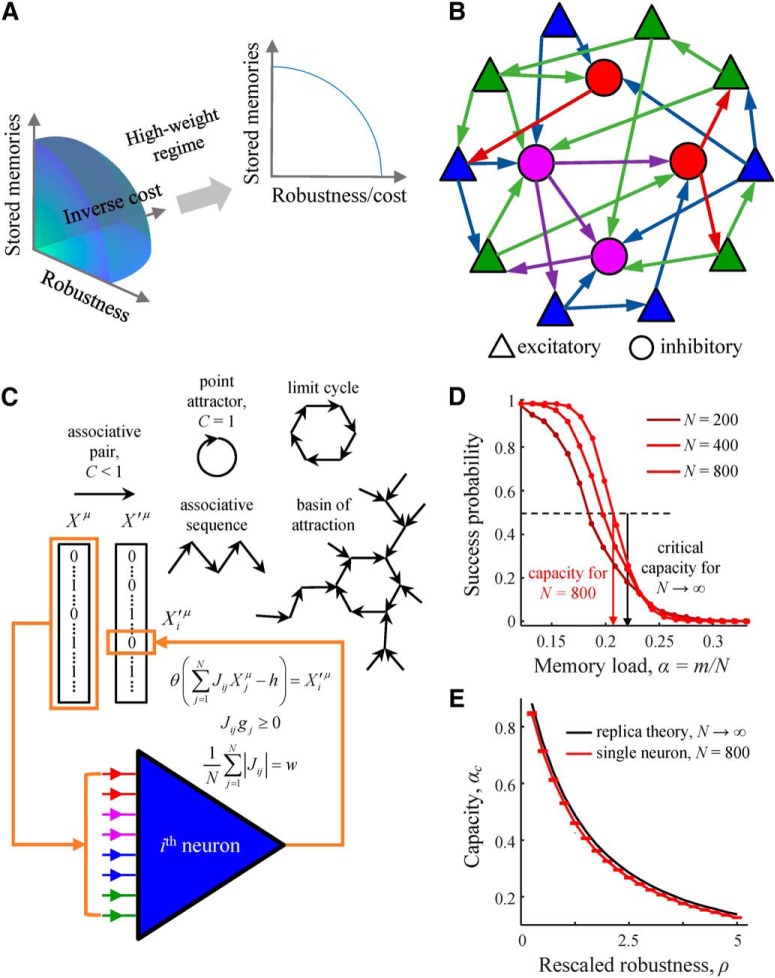
With sensory information continuously impinging on the brain, neural circuits function in a state of perpetual change, recording some of the information in the form of long-term memories. During the learning process, individual neurons may be operating as independent learning units, constrained by functional and metabolic considerations, such as the requirement to store associative memories, tolerate noise during memory retrieval, and maintain a low cost of the underlying connections (see Fig. 1A). In this study, we explore the structural and dynamical properties of associative networks in the space of these constraints and show that there is a unique region of parameters that can explain the above-described experimental observations.

Figure 1.

Associative memory storage in recurrent networks of excitatory and inhibitory neurons. A, Associative learning in the brain is expected to be constrained by functional and metabolic considerations, such as being able to store large amounts of memories, tolerate noise during memory retrieval, and have a low cost of the underlying connectivity. In the model, these three considerations are represented with memory load, α, robustness parameter, κ, and average absolute connection weight, w. We show that, in the biologically plausible regime of high weight, results of the model depend only on α and κ/w. B, Recurrent network of various classes (color) of all-to-all potentially connected excitatory and inhibitory neurons. Arrows indicate actual (or functional) connections. C, Associative memory in the model is a connected graph of successive network states (directed edges termed associations), {X^μ→X′^μ}, in which every node has no more than one daughter node. Each neuron in the network (e.g., neuron i) must learn a set of input–output associations derived from the memory (orange boxes) by modifying the strengths of its input connections, J_ij, under the constraints on connection signs and l₁-norm. D, A neuron's ability to learn a presented set of associations decreases with the number of associations in the set, m. The memory storage capacity of the neuron, α_c (e.g., red arrow for N = 800) is defined as the fraction of associations, m/N, that can be learned with success probability of 50%. The transition from perfect learning to inability to learn the entire set of associations sharpens with increasing N and approaches the result obtained with the replica theory in the limit of N → ∞ (black arrow). Results shown correspond to associative sequences of uncorrelated network states, C = 0. Numerical results for N = 200, 400, and 800 were obtained with convex optimization (lines) and the modified perceptron learning rule (dots) (for details, see Materials and Methods). E, The capacity of a single neuron is a decreasing function of the rescaled robustness, ρ. Error bars indicate SDs calculated based on 100 networks.

Materials and Methods

Associative learning model for networks of biologically constrained excitatory and inhibitory neurons.

We use a McCulloch and Pitts neural network (McCulloch and Pitts, 1943) to model a local cortical circuit in which N_inh inhibitory neurons and (N − N_inh) excitatory neurons are all-to-all potentially connected (Stepanyants and Chklovskii, 2005; Stepanyants et al., 2008) (see Fig. 1B). Associative memory in the model is a connected graph of successive network states (directed edges termed associations), {X^μ→X′^μ}, in which every node has no more than one daughter node (see Fig. 1C). Vectors X^μ and X′^μ contain binary activities (0 or 1) of individual neurons within an association μ. In general, an associative memory can be in the form of a point attractor, an associative sequence, a limit cycle, and an entire basin of attraction. However, because the precise format of associative memories in cortical networks is not known, in the following, we first examine memories composed of uncorrelated network states and then extend the analysis on a specific class of memories with correlations. The first case excludes memories that contain point attractors and limit cycles, which necessarily include correlations; and aside from this restriction, the results are independent of the specifics of memory structures. In all numerical simulations of this case, we use memories in the form of associative sequences. In the second case, we only consider a specific format in which a memory is composed of pairs of correlated associative network states and vary the correlation coefficient, C, in the 0–1 range. We note that, at C = 0, we recover the results of the first case; and at C = 1, the associative pairs are in the form of point attractors (Hopfield, 1982).

Learning in the network is mediated by changes in connection weights of individual neurons, J_ij, in the presence of several biologically inspired constraints. (1) Input connection weights of each neuron are sign-constrained to be non-negative if the presynaptic neuron is excitatory and nonpositive if it is inhibitory (Dale's principle) (Dale, 1935). We note that violations of Dale's principle have been reported in some cortical systems under extreme conditions, such as prolonged seizures (Spitzer, 2017), but there is no strong evidence to suggest that widespread deviations from this principle occur under normal behavioral conditions. (2) Input weights of each neuron are homeostatically constrained to have a predefined l₁-norm (Holtmaat et al., 2006; Bourne and Harris, 2011; Kim and Nabekura, 2011; El-Boustani et al., 2018). (3) Each neuron must attempt to learn its associations robustly so that they can be recalled correctly in the presence of a given level of postsynaptic noise. Biological motivations and assumptions of this model have been previously described (Chapeton et al., 2015).

Each neuron in the network (e.g., neuron i), independently from other neurons, attempts to learn a set of input–output associations {X^μ→X′^μ_i}, in which a vector X^μ represents the neuron's input for an association μ, and a scalar X′^μ_i is the desired output of the neuron derived from the subsequent network state X′^μ (see Fig. 1C, orange boxes). To simplify the notation, in the following, we drop index i, replace X′^μ_i with y^μ, and summarize the learning problem, such as the following:

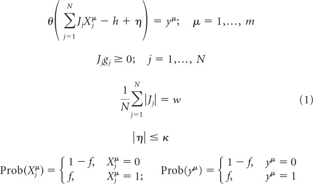In these expressions, θ denotes the Heaviside step-function, h is the neuron's firing threshold, and η denotes its postsynaptic noise, which is bounded by the robustness parameter κ, i.e., |η| < κ. To enforce sign constraints on the neuron's presynaptic connection weights, we introduce a set of parameters {g_j} and set g_j to 1 if connection j is excitatory and −1 if it is inhibitory. Parameter w, referred to as the average absolute connection weight, is introduced to impose the l₁-norm constraint on the weights of these connections. Binary input and output states, X_j^μ and y^μ, are randomly drawn from the Bernoulli probability distribution: 0 with probability 1 − f and 1 with probability f.

The above network model is governed by the following parameters: number of neurons in the network (N), fraction of inhibitory neurons (N_inh/N), threshold of firing (h), firing probability of neurons in the associative states (f), average absolute connection weight (w), robustness parameter (κ), and memory load (α = m/N).

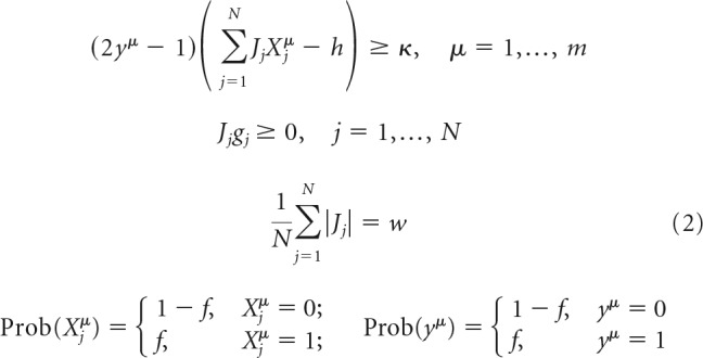
The first line in Equation 1 can be rewritten as an inequality, (2y^μ − 1)(∑_j=1^NJ_jX_j^μ − h + η) ≥ 0, making it possible to eliminate η and rewrite the problem in a more concise form as follows:

Numerical solution of the model.

The solution of Equation 2 can be obtained numerically with the methods of convex optimization (Boyd and Vandenberghe, 2004). In numerical simulations, we consider two learning scenarios: (1) feasible load, in which associations can be learned given the constraints of the problem; and (2) nonfeasible load, in which the number of presented associations is so large that Equation 2 has no solution.

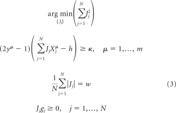
In the feasible load scenario, the region of solutions is nonempty, and one must use additional considerations to limit the results to a single, “optimal” solution. We do this by choosing the solution that minimizes ‖J‖₂², as follows:

In the nonfeasible scenario, similar to what is done in the formulation of the support vector machine problem (Hastie et al., 2009), we introduce a slack variable s^μ ≥ 0 for every association to make the learning problem feasible and choose the solution that minimizes the sum of these variables by solving the following linear optimization problem:

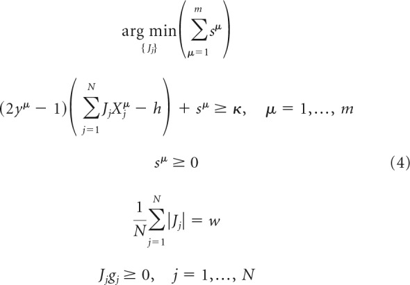The problems outlined in Equations 3 and 4 were solved in MATLAB in the following sequence of steps. Given the associative memory load, α = m/N, we first solved the problem of Equation 4, using the linprog function, to find s^μ. If any of these slack variables are >0, the problem is nonfeasible. If all s^μ = 0, the problem is feasible, in which case we used the connection weights resulting from Equation 4 as a starting configuration and solved Equation 3 with the quadprog function. In running linprog and quadprog functions, we adopted the primal-dual interior-point algorithm (Altman and Gondzio, 1999) to find the minima of the objective functions in Equations 3 and 4 under the linear inequality and equality constraints. This algorithm solves the regularized optimization problem in the dual space by using Newton's method (Boyd and Vandenberghe, 2004).

In addition to the convex optimization solutions described with Equations 3 and 4, we developed a more biologically plausible solution of the associative learning problem by modifying the perceptron learning rule (Rosenblatt, 1962). In this rule, a single not yet robustly learned association is chosen at random and the synaptic weights of the neuron are updated in four consecutive steps as follows:

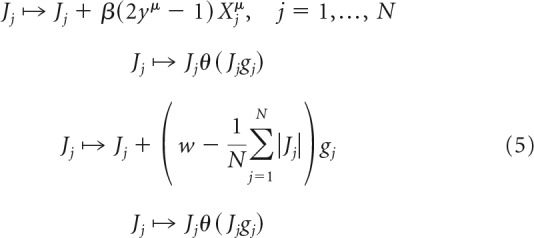Unlike the standard perceptron learning rule, Equation 5 enforces the sign and homeostatic l₁-norm constraints during learning. A closely related rule, in the absence of l₁-norm constraint, was previously described (Brunel et al., 2004; Clopath et al., 2012). The first update in Equation 5 is a standard perceptron learning step, in which parameter β is referred to as the learning rate. The second step is introduced to enforce the sign constraints, whereas the last two steps combined implement the homeostatic l₁-norm constraint and are equivalent to the soft thresholding used in LASSO regression (Tibshirani, 1996). We note that, although the robustness parameter κ does not explicitly appear in Equation 5, the rule implicitly depends on the value of this parameter. This is because the update of connection weights is triggered by the presentation of not robustly learned associations (i.e., associations violating the first inequality of Eq. 2), the definition of which is dependent on κ. In all numerical simulations, we set β = 0.01 and ran the algorithm until a solution was found or the maximum number of iterations of 10⁷ was reached. Figure 1D shows that the success probability and memory storage capacity calculated based on the modified perceptron learning rule (dots) are nearly identical to the results obtained with convex optimization (lines).

MATLAB code for generating replica theory and numerical solutions of the associative model is available at https://github.com/neurogeometry/AssociativeLearning.

Replica theory solution of the model in the N → ∞ limit.

This section outlines the replica theory (Edwards and Anderson, 1975; Sherrington and Kirkpatrick, 1975) solution of Equation 2. The complete derivation is described by Zhang et al. (2018). Solutions of related models, which include only some of the constraints of this study and consider a specific scaling of connection weights with N, can be found in these studies (Gardner and Derrida, 1988; Brunel et al., 2004; Chapeton et al., 2012, 2015; Brunel, 2016; Rubin et al., 2017). In the following, we assume that N is large, whereas m/N and f are O(1) (of order 1 with respect to N). The total postsynaptic input to the neuron can be expressed in terms of its average over the input network states, {X^μ}, plus a deviation from the average as follows:

With this, the associative learning problem of Equation 2 can be separated into two categories based on the value of y^μ as follows:

To guarantee O(1) capacity in the large N limit, it is necessary for the deviation of the average postsynaptic input from the threshold, f∑_j=1^NJ_j − h, and the robustness parameter, κ, to be of the same order as (or less than) the SD of the postsynaptic input distribution, σ_input = $\sqrt{f\left(1-f\right){\displaystyle {\sum }_{j=1}^N{J}_j^2}}$. If not, input to the neuron will rarely cross the threshold (if the first condition is violated) or the robustness margins (if the second condition is violated), and capacity for robust associative memory storage will be close to zero. Therefore,

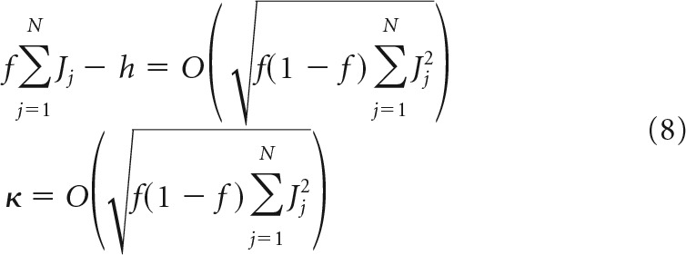Equation 8 gives rise to various plausible scenarios for scaling of the connection weights and robustness parameter with the network size as follows:

The normalized weights, J̃_j, and the normalized robustness parameter, κ̃, in Equation 9 do not scale with N.

The first scenario (first terms in braces in Eq. 9) is usually used in associative memory models in conjunction with the replica theory (see, e.g., Brunel et al., 2004) as follows:

The second scaling scenario is traditionally used in balanced network models (see, e.g., Rubin et al., 2017) as follows:

The third and the subsequent scenarios, in which J does not scale with N, or J increases with N, can be ruled out because they are biologically unrealistic. In addition, one can see from Equation 2 that the firing threshold in these cases can be disregarded, and the results of replica calculation become identical to the second scaling scenario.

In all models, scaling of w is assumed to be the same as that of J; that is, w = $\left\{\frac{1}{N},\frac{1}{\sqrt{N}}\right\}\tilde{w}h$. Substituting the normalized variables into Equation 2, we arrive at two problems, both governed by the same set of intensive parameters, f, κ̃, w̃, g_j, and extensive parameters m and N as follows:

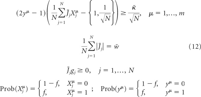The two formulations only differ in the threshold term (braces). We solve the two models concurrently (Zhang et al., 2018) and obtain the neuron's critical (maximum) capacity, α, probabilities of excitatory and inhibitory connections, P_exc/inh^con, and probability densities of non-zero excitatory and inhibitory connection weights, P_exc/inh^PSP as follows:

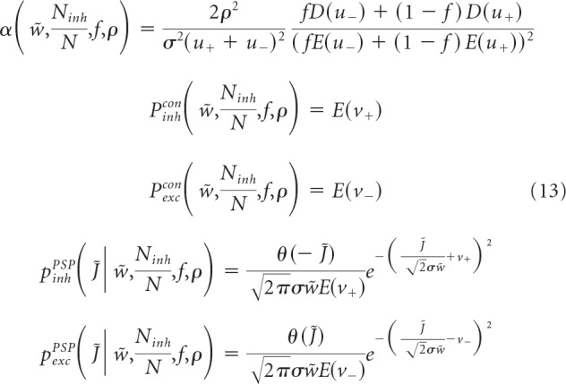These quantities are expressed as functions of five latent variables, u₊, u₋, ν₊, ν₋, and σ, which can be obtained by solving the following system of equations and inequalities:

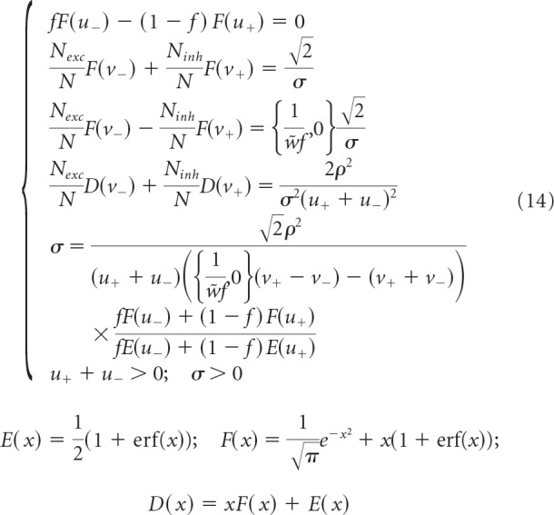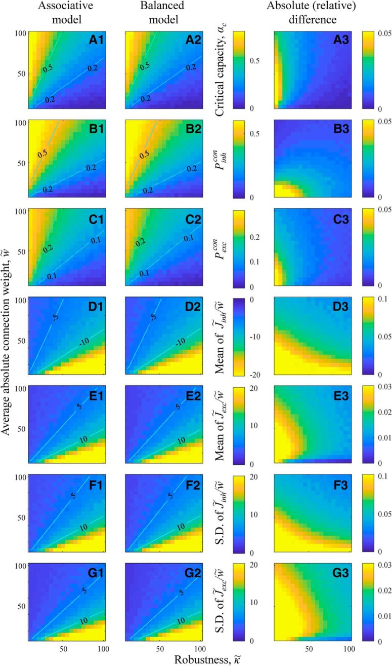
We note that the distributions of inhibitory and excitatory connection weights are composed of Gaussian functions (SD σ) truncated at zero and finite fractions of zero-weight connections. The difference between the replica solutions of the associative and balanced models explicitly appears only in lines 3 and 5 of Equation 14, which contain braces. The first and second terms in these braces correspond to the associative and balanced solutions, respectively. Equation 14 makes it clear that the solution of the associative model in the high-weight limit, w̃f >> 1, converges to the solution of the balanced model. However, since the value of w̃f estimated from experimental data is large but finite (see Results), we also examined the agreement between the results of the two models by solving Equations 13 and 14 numerically for different values of w̃ and κ̃. Figure 2 shows that, for values of w̃ in the 10–100 range, the results of the two models agree within 10%, and the agreement improves with increasing κ̃. In addition, in the limit of high weight, the solution depends only on κ̃/w̃ (Fig. 2, straight isocontour lines). Therefore, instead of κ̃, we use parameter ρ = $\frac{\tilde{\kappa }}{\tilde{w}\sqrt{f\left(1-f\right)}}$, which was introduced by Brunel et al. (2004) and Brunel (2016) and is referred to as the rescaled robustness. This parameter can serve as a proxy for the ratio of robustness and SD of postsynaptic input, κ/σ_input.

Figure 2.

Replica theoretical solutions for the associative and balanced models converge in the limit of w̃f >> 1. In this limit, model results depend only on κ̃/w̃, in agreement with Equations 13 and 14. A, Maps of critical capacity as functions of κ̃ and w̃ for the associative (A1) and balanced (A2) models. Straight isocontours confirm that the results depend only on κ̃/w̃. The absolute difference of the two maps (A3) shows that critical capacities of the two models converge in the limit of w̃f >> 1. Same for the probabilities of inhibitory (B) and excitatory (C) connections. D, Maps of mean, non-zero, inhibitory connection weights as a function of κ̃ and w̃ for the associative (D1) and balanced (D2) models, as well as the absolute relative difference of these maps (D3). Same for the mean, non-zero, excitatory connection weights (E), and SDs of non-zero inhibitory (F) and excitatory (G) connection weights.

We note that since $\frac{\tilde{\kappa }}{\tilde{w}}=\frac{\kappa }{w\sqrt{N}}$ for both models, rescaled robustness, ρ, and Equations 13 and 14 in the high-weight limit are model independent. The fact that the solutions of the two models converge in the high-weight regime is not surprising. In this regime, Nwf >> h, and, as a result, mean excitatory and inhibitory inputs to the neuron are much greater than the threshold of firing. One can show that, in this case, h in Equation 2 can be disregarded, and the solution becomes independent of scaling of J with N. Figure 3 shows that, with increasing N, numerical solutions of the model according to Equations 3 and 4 gradually approach the results of the replica theory outlined in Equations 13 and 14. This agreement serves as an independent validation of the numerical and theoretical calculations.

Figure 3.

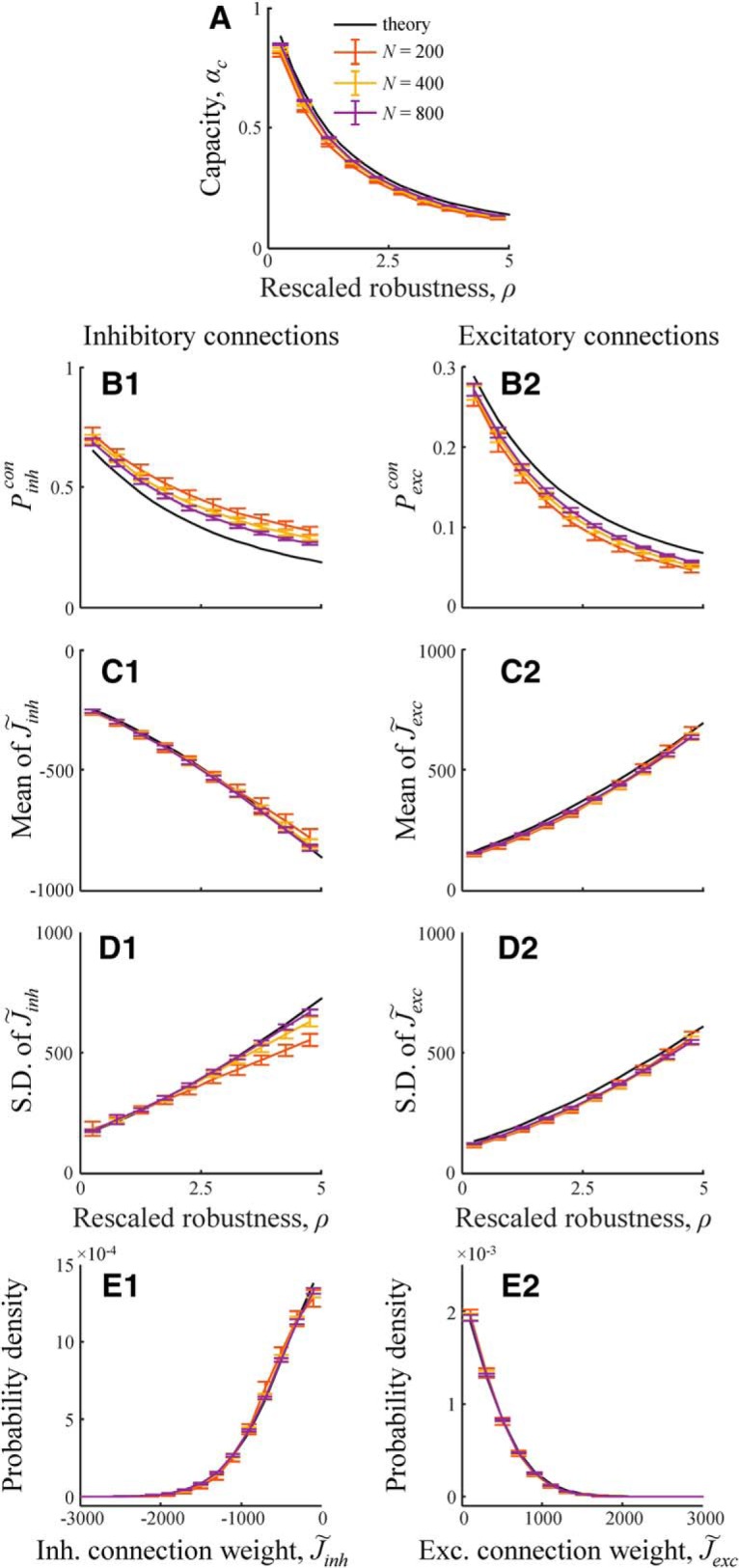
Validation of the theoretical results of Equations 13 and 14 with numerical simulations performed for N = 200, 400, and 800 inputs. A, Capacity as a function of rescaled robustness, ρ. With increasing N, numerical results (error bars) obtained with convex optimization, Equations 3 and 4, approach the theoretical solution (black line). Error bars indicate SDs calculated based on 100N simulations. Same for the probabilities of non-zero inhibitory (B1) and excitatory (B2) connections, mean non-zero inhibitory (C1) and excitatory (C2) connection weights, and SDs of non-zero inhibitory (D1) and excitatory (D2) connection weights. E1, E2, The match between theoretical and numerical probability densities of non-zero inhibitory and excitatory connection weights for ρ = 1.

Results

Network model of associative learning

We use a McCulloch and Pitts neural network (McCulloch and Pitts, 1943) to model a local cortical circuit in which N_inh inhibitory neurons and (N − N_inh) excitatory neurons are all-to-all potentially connected (Stepanyants and Chklovskii, 2005; Stepanyants et al., 2008) (Fig. 1B). Associative memories are loaded into the network by modifying the weights of connections between neurons (for details, see Materials and Methods). Associative memory in the model is a connected graph of successive network states, which in general, can be in a form of a point attractor, an associative sequence, a limit cycle, and an entire basin of attraction (Fig. 1C). The precise format of associative memories in cortical networks is not known and is likely to be area dependent. Yet, for uncorrelated network memory states (which excludes point attractors and limit cycles), the format of memories has no effect on network properties, and this is the case we consider first.

During learning, individual neurons, independently from one another, attempt to associate inputs and outputs derived from the associative memory states (Fig. 1C). Several biologically motivated constraints are imposed on the learning process (Chapeton et al., 2015). First, firing thresholds of neurons, h, do not change during learning. Second, the signs of input weights, J, that are determined by the excitatory or inhibitory identities of presynaptic neurons, do not change during learning (Dale's principle) (Dale, 1935). Third, input connections of each neuron are homeostatically constrained to have a fixed average absolute weight, w (Holtmaat et al., 2006; Bourne and Harris, 2011; Kim and Nabekura, 2011). Fourth, each neuron must be able to retrieve the loaded associations, even in the presence of noise in its postsynaptic potential. The maximum amount of noise a neuron has to tolerate is referred to as robustness parameter, κ.

Individual neurons in the model attempt to learn the presented set of associated network states, and the probability of successfully learning the entire set decreases with the memory load, α (Fig. 1D). Memory load that can be successfully learned by a neuron with the probability of 0.5 is termed the associative memory storage capacity of the neuron, α_c. This capacity increases with the number of neurons in the network, N, and saturates in the N → ∞ limit at a value that can be determined with the replica theory (see Materials and Methods). Notably, this theoretical solution shows that, in the high-weight regime (Nwf/h >> 1), the neuron's capacity, as well as the shape of its connection weight distribution, depend on the combination of model parameters in the form of ρ = $\frac{\kappa }{w\sqrt{Nf\left(1-f\right)}}$ (Figs. 1A, 2). The meaning of this combination was elucidated by Brunel et al. (2004), where it was pointed out that ρ can be viewed as a measure of reliability of stored associations to errors in the postsynaptic input. Following Brunel (2016), we refer to ρ as the rescaled robustness.

Motivated by this theoretical insight, we set out to explore the possibility that local networks in the brain function in the high-weight regime. The average absolute connection weight, w, was previously estimated based on experimental data from various cortical systems (Chapeton et al., 2015), and the result shows that Nwf/h lies in the range of 4–38 (95% CI) with the average of 14. A similar estimate based on the granule to Purkinje cell connectivity in rat cerebellum (Brunel et al., 2004) also results in a relatively high value of this parameter, Nwf/h ≈ 150,000 × 0.1 mV × 0.0044/10 mV = 6.6. Therefore, the high-weight regime may be a general attribute of local circuits, and we show that this assumption is consistent with many experimental measurements related to network structure and dynamics.

As was previously inferred from experimental observations (Chapeton et al., 2015), in the following, we set the fraction of inhibitory neurons to N_inh/N = 0.2, the firing probability to f = 0.2, and Nwf/h = 14 (high-weight regime). In this regime, structural and dynamical properties of associative networks depend primarily on rescaled robustness and memory load; and in the following, we examine the network properties as functions of these two parameters. Figure 1E shows that the memory storage capacity of a single neuron is a decreasing function of rescaled robustness. This is expected, as an increase in ρ can be thought of as an increase in the strength of the constraint on learning (robustness, κ) or as a decrease in available resources (absolute connection weight, w). With increasing N, solutions gradually approach the results of the replica theory, which serves as an independent validation of numerical and theoretical calculations (Fig. 3).

Statistics of synaptic connections in the brain and in associative networks

We examined the properties of neuron-to-neuron connectivity in associative networks at different values of rescaled robustness and memory load. One of the most prominent features of connectivity is that substantial fractions of excitatory and inhibitory connections have zero weights (Brunel et al., 2004; Chapeton et al., 2015); and therefore, connection probabilities are <1 (Fig. 4A). One can intuitively explain the presence of a finite fraction of zero-weight connections by considering a learning process during which inhibitory and excitatory connections change weights. Over time, many weights will approach zero and accumulate there, unable to pass it due to sign constraints. The distributions of non-zero connection weights in associative networks resemble the general shapes of unitary postsynaptic potential distributions, with a notable difference in the frequencies of very strong connections. The former have Gaussian or exponential tails (Brunel et al., 2004; Chapeton et al., 2015), whereas the tails of unitary postsynaptic potential distributions are often much heavier (Song et al., 2005; Lefort et al., 2009). Several amendments to the associative model have been proposed to account for this discrepancy (Brunel et al., 2004; Chapeton et al., 2012). Here, we would like to point out that heavy tails of experimental distributions can be reproduced within the associative model by considering networks of neurons with heterogeneous properties (e.g., different values of w and/or κ).

Figure 4.

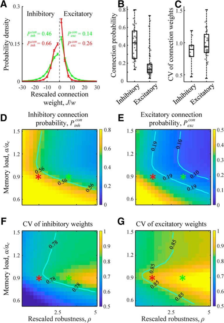
Properties of neuron-to-neuron connectivity in associative networks. A, Distributions of weights of inhibitory and excitatory connections for two-parameter settings (D–G, red and green asterisks). The distributions contain finite fractions of zero-weight connections. Error bars indicate SDs (based on 100 networks). B, C, Experimentally measured connection probabilities and CVs of connection weights for inhibitory and excitatory connections in mammals (Figure 4-1). Each dot represents the result of a single study averaged (with weights equal to the number of connections tested) over the number of reported projections. Maps of probabilities of inhibitory (D) and excitatory (E) connections as functions of rescaled robustness and relative memory load (i.e., load divided by the theoretical single-neuron capacity at N → ∞). Inhibitory connection probability is higher than the probability of excitatory connections in the entire region of considered parameters. F, G, Maps of CVs of non-zero inhibitory and excitatory connection weights as functions of rescaled robustness and relative memory load. Isocontour lines in the maps indicate the interquartile ranges of experimentally observed connection probabilities and CVs shown in B and C. A, D–G, Numerical results were obtained with convex optimization based on networks of N = 800 neurons.

Figure 4-1

Dataset of connection probabilities and strengths in local brain circuits in mammals. The dataset is a compilation of 87 articles published in peer-reviewed journals from 1990 to 2016, describing a total of 420 projections. Download Figure 4-1, XLSX file ^{(68.2KB, xlsx)}

To compare connection probabilities and widths of non-zero connection weight distributions in associative networks with those reported experimentally, we compiled experimental measurements published in peer-reviewed journals since 1990. Initially, we identified 152 articles describing a total of 856 projections. Later we limited our analyses to experiments in which recordings were made in the neocortex, from at least 10 pairs of neurons located in the same layer and separated laterally by <100 μm. We also limited the analyses to normal, juvenile or adult animals (no younger than P14 for mouse and rat, and older than that for ferret, cat, monkey, and human). After imposing these limits, the numbers of publications and projections reduced to 87 and 420, respectively (see Fig. 4-1).

Figure 4B, C shows that the average inhibitory connection probability (based on 38 studies, 9522 connections tested) is significantly higher (p < 10⁻¹⁰, two-sample t test) than the average probability for excitatory connections (67 studies, 63,020 connections tested), whereas CV of inhibitory unitary postsynaptic potentials (10 studies, 503 connections recorded) is slightly lower than that for excitatory (36 studies, 3956 connections recorded). Similar trends are observed in associative networks. Figure 4D, E shows that connectivity in associative networks is sparse, with probabilities of excitatory non-zero connections lower than those for inhibitory connections in the entire considered range of rescaled robustness and relative memory load. Probabilities of both connection types are decreasing with increasing ρ. This is expected because an increase in ρ can be achieved by lowering w, which is equivalent to limiting the resources needed to make connections. Isocontours in Figure 4D, E demarcate the interquartile ranges of connection probability measurements shown in Figure 4B. There is a region in the α-ρ space of parameters in which both excitatory and inhibitory connection probabilities are in general agreement with the experimental data. Also, consistent with the experimental measurements, CVs of excitatory weights in associative networks are slightly larger than those for inhibitory weights (Fig. 4F,G), and there is a wide region in the α-ρ space of parameters in which these values match the experimental data shown in Figure 4C.

Properties of 2- and 3-neuron motifs in associative networks

We also compared the statistics of 2-neuron motifs in associative and cortical networks. Figure 5A shows that the numbers of bidirectionally connected pairs of excitatory neurons do not significantly deviate from those observed in shuffled networks, and the overexpression of bidirectional connections is close to 1 in the entire considered range of rescaled robustness and relative memory load. The same result was reported by Brunel (2016) for associative memories composed of uncorrelated network states. In agreement with this finding, Lefort et al. (2009) reported no overexpression in barrel cortex (8895 recorded connections in layers 2–6). However, several other studies reported significantly >1 overexpression ratios. This ratio was found to be 2 in visual cortex (340 recorded connections) (Wang et al., 2006), 3 in somatosensory cortex (1380 recorded connections in layer 5) (Markram et al., 1997), 3 in visual and somatosensory cortex (1084 recorded connections in L2/3) (Holmgren et al., 2003), 4 in prefrontal cortex (1233 recorded connections) (Wang et al., 2006), and 4 in visual cortex (8050 recorded connections in layer 5) (Song et al., 2005). We show that the observed 1–4 range of overexpression ratios can result from associative memories formed by correlated pairs of network states (see Effect of correlations on structure and dynamics of associative networks).

Figure 5.

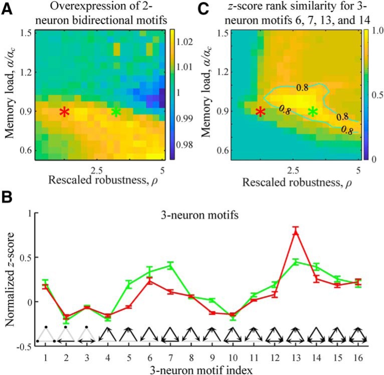
Two- and three-neuron structural motifs in associative networks. A, Map of the overexpression ratios for bidirectional excitatory 2-neuron motifs shows no significant deviation from 1 in the entire range of the considered rescaled robustness and relative memory load. B, Normalized z scores of 16 3-neuron motifs in excitatory subnetworks indicate overexpression and underexpression of these structures compared with the chance levels. Red and green curves indicate the results for the parameter settings specified by the red and green asterisks in A. Error bars indicate SDs. C, Average fraction of excitatory 3-neuron motifs 6, 7, 13, and 14 appearing in associative networks among the top four z score motifs. Isocontour line, indicating the region of reasonably good solutions, is drawn as a guide to the eye. Results were generated based on 100 networks of N = 800 neurons.

In addition to specific properties of neuron-to-neuron connectivity, local cortical circuits are known to have nonrandom patterns of connections in subnetworks of three and more neurons (Song et al., 2005; Perin et al., 2011; Rieubland et al., 2014). To determine whether associative networks can reproduce some of the known features of higher-order connectivity, we first examined the statistics of connectivity motifs within subnetworks of three excitatory neurons. There are 16 distinct types of 3-neuron motifs (Fig. 5B, inset). Frequencies of these motifs in subnetworks of excitatory neurons, n_i, were calculated with the Brain Connectivity Toolbox (Rubinov and Sporns, 2010) and compared with the corresponding frequencies in networks in which connections were randomly shuffled in a way that preserves the numbers of 2-neuron motifs, n_i^shuffled. We used normalized z scores, z_i^norm, as defined by Gal et al. (2017), to characterize the degrees of overexpression and underexpression of motif types as follows:

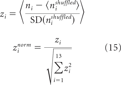Here, outer angle brackets in the first equation denote averaging over 100 associative networks, whereas angle brackets in the numerator and SD in the denominator represent the average and SD calculated based on a set of 50 randomly shuffled versions of a given associative network. Normalized z scores lie in the range of −1 to 1 and are negative/positive for motifs that appear less/more frequently than what is expected by chance.

Figure 5B shows the profiles of normalized z scores in associative networks configured at the values of rescaled robustness and relative memory load defined by the red and green asterisks from Figure 4. Both curves show overexpression of motifs 6, 7, 13, and 14, in agreement with previous data (Song et al., 2005; Perin et al., 2011). In particular, Perin et al. (2011) have high enough counts to show that these specific motifs are significantly overexpressed (p < 0.01) and have the highest z scores. To check whether the same is true in associative networks, we calculated the average fraction of these motifs in the top-four z score group. Figure 5C shows that this fraction is maximal in the parameter region near the green asterisk. Within the region outlined by the isocontour line, this fraction is >0.8, indicating that, in associative networks, >3.2 motifs on average of motifs 6, 7, 13, and 14 appear in the top-four z score group.

One can justify the overexpression of motifs 6, 7, 13, and 14, by following the reasoning outlined by Brunel (2016) for bidirectional connections. According to the perceptron learning rule, a change in connection weight from neuron j to neuron i is driven by a coactivation of memory states X_j^μ and X_i^′μ. As a result, convergent connections onto neuron i (and divergent connections from neuron i) end up correlated because they are driven by a common memory state, X_i^′μ (and X_i^μ). In general, 3-neuron motifs dominated by convergent and divergent connections are expected to be overexpressed; however, the exact value of the overexpression ratio is difficult to predict as it depends on rescaled robustness and memory load.

Higher-order structural properties of associative networks

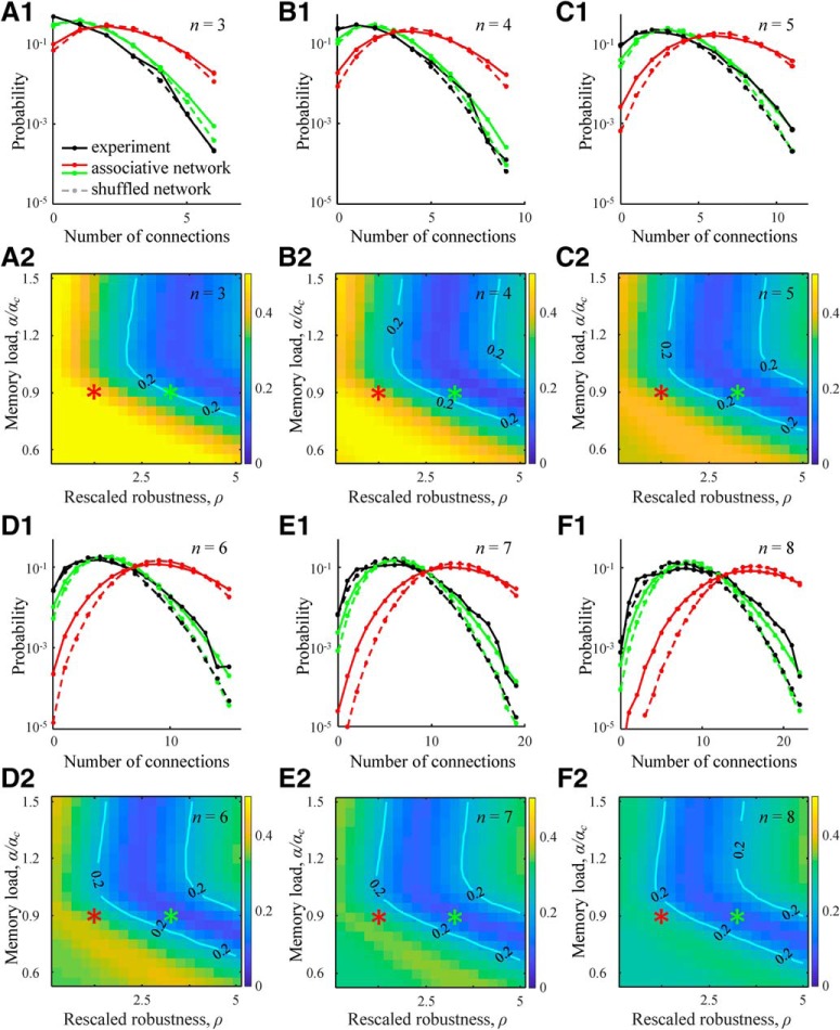
Deviations from random connectivity have also been detected in subnetworks of 3–8 excitatory neurons by comparing distributions of observed connection numbers with those based on randomly shuffled connectivity (Perin et al., 2011). This comparison revealed that the experimental distributions can have heavier tails indicative of clustered connectivity (e.g., Fig. 6F1, black line). This trend was first reproduced by Brunel (2016) who considered an associative network of excitatory neurons at capacity. The same trend is present in our model in the parameter region near the green asterisk (Fig. 6, green lines). In addition, our results show that there is a single region of parameters α and ρ in which the tails of the experimental distributions are reproduced simultaneously for all subnetworks from 3 to 8 neurons. We note that there are network models that can produce nonrandom connectivity, including motifs and clustering, by directly tuning parameters governing network structure (Vegué et al., 2017). This, however, significantly differs from the approach described in this study, which relates the structural features of connectivity to the functional requirement of robust associative memory storage.

Figure 6.

Distributions of non-zero connection numbers in clusters of 3–8 excitatory neurons in associative networks. A1–F1, Solid red and green lines indicate distributions obtained in associative networks for the parameter settings indicated by the red and green asterisks. Solid black curves indicate the corresponding results for local cortical networks based on electrophysiological measurements (Perin et al., 2011). Dashed lines indicate distributions in randomly shuffled networks. Distributions of non-zero connection numbers in clusters of 3–8 excitatory neurons in associative networks are significantly different from the corresponding distributions in randomly shuffled networks (20,000 subnetworks, two-sample Kolmogorov–Smirnov test, p < 10⁻⁷). A2–F2, Maps of l₂ distances between the logarithms of connection number probabilities in associative and cortical subnetworks of 3–8 neurons. Numerical results were generated based on 100 networks of N = 800 neurons.

Dynamical properties of spontaneous activity in associative networks

To quantify spontaneous dynamics in an associative network, we initialized the network at a random state of firing probability f = 0.2 and followed the network activity until it terminated at an attractor or a limit cycle. We did not explicitly prohibit the initialization of the network at or close to one of the αN learned memory states since the probability of such a coincidence in large networks (N = 800) is exponentially small. Similarly, because the number of available network states is much larger than the number of learned states, spontaneous network activity is not expected to pass through any of the learned states. Indeed, we did not observe such an event in any of the 10⁴ numerical simulations (100 networks, 100 starting points for each network). Spontaneous dynamics of associative networks depends strongly on the values of rescaled robustness and relative memory load. At small values of ρ, network dynamics quickly terminates at a fixed point in which all neurons are silent (Fig. 7A1, red). When ρ is high, associative networks can have long-lasting intrinsic activity, often ending up in a limit cycle of non-zero length. To quantify this behavior, we measured the average number of steps taken by the network to reach a limit cycle or a fixed point (Fig. 7A2). The results show that the duration of transient dynamics increases exponentially with rescaled robustness and memory load. Even for moderate values of these parameters, the average length of transient activity can be of the order of network size, N (Fig. 7A2, contour).

Figure 7.

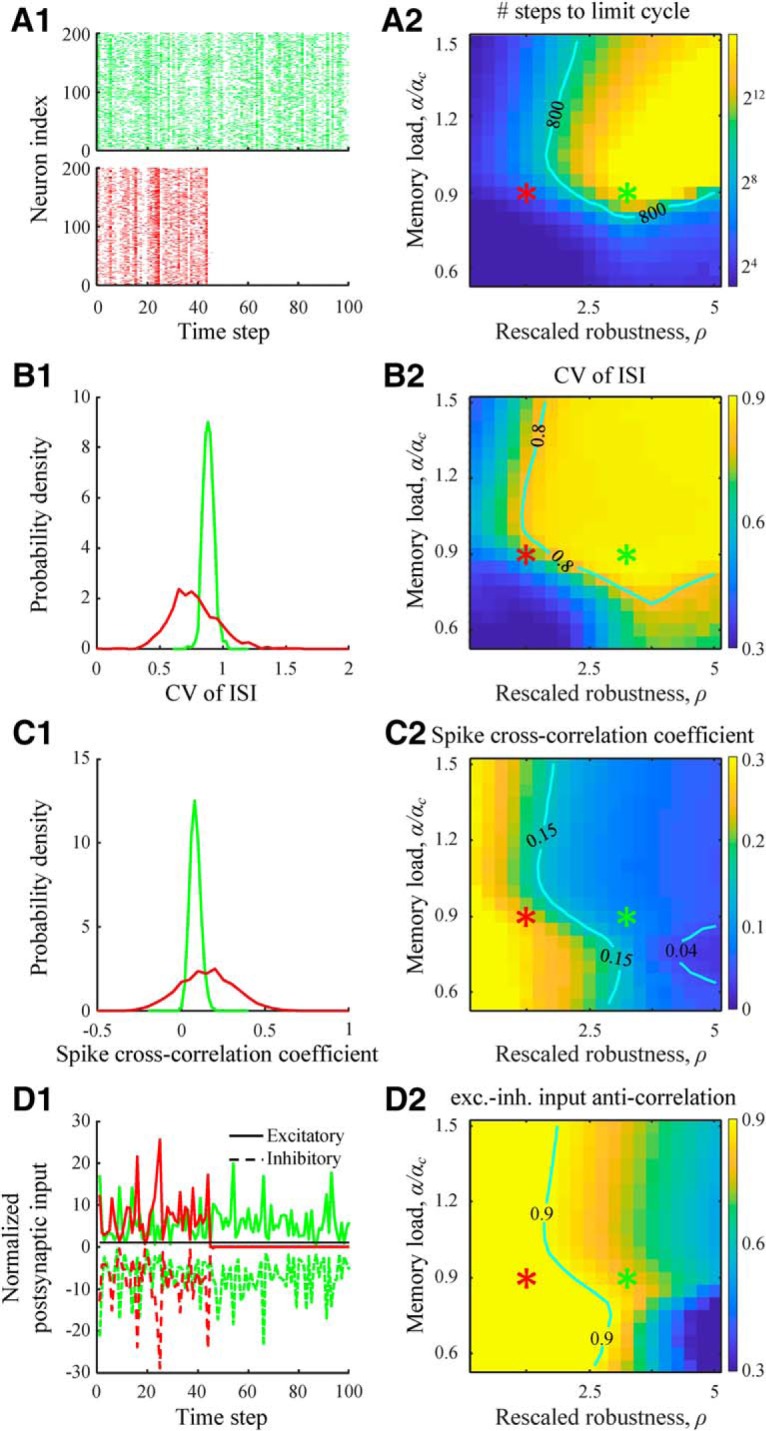
Dynamical properties of spontaneous activity in associative networks. A1, Two examples of spike rasters for associative networks parametrized as indicated by the red and green asterisks from A2. Dynamics at low values of rescaled robustness (red) quickly terminates at a quiescent state. A2, Map of the duration of transient dynamics as a function of rescaled robustness and relative memory load. At high levels of rescaled robustness and memory load, associative networks have long-lasting, transient activity. Isocontour line is drawn as a guide to the eye. B1, Distributions of CV in ISIs for the two parameter settings. The average CV value increases with ρ. B2, Map of the average CV of ISI as a function of rescaled robustness and relative memory load. Isocontour line indicates a region of high CV values that are in general agreement with experimental measurements. C, Same for cross-correlation coefficients of neuron spike trains. D, Same for the anticorrelation coefficient of excitatory and inhibitory postsynaptic inputs received by a neuron. The inputs are normalized by the firing threshold. For the selected parameter configurations, excitatory and inhibitory inputs are tightly balanced (large anticorrelation) despite large fluctuations. A2, B2, C2, D2, Maps were generated based on networks of N = 800 neurons by averaging the results over 100 networks and 100 random initial states for each network and parameter setting.

Individual neurons in associative networks can produce irregular spiking activity, the degree of which can be quantified with a CV of ISIs (Fig. 7B). According to this measure, neurons exhibit greater irregular activity when rescaled robustness and memory load are high, with a CV of ISI values saturating at ∼0.9. This is consistent with the range of CV of ISI values reported for different cortical systems (0.7–1.1) (Softky and Koch, 1993; Holt et al., 1996; Buracas et al., 1998; Shadlen and Newsome, 1998; Stevens and Zador, 1998). To examine the extent of synchrony in neuron activity, we calculated spike train cross-correlation coefficients for pairs of neurons (Fig. 7C). The results show that increase in ρ leads to a more asynchronous activity, which can be explained by the reduction in connection probability (Fig. 4D,E) and, consequently, reduction in the amount of common input to the neurons. For ρ > 2.5, the cross-correlation values are consistent with experimental data (0.04–0.15; interquartile range derived from 26 studies) (Cohen and Kohn, 2011).

An irregular, asynchronous activity can result from a balance of excitation and inhibition (van Vreeswijk and Sompolinsky, 1996, 1998). In the balanced state, the magnitudes of excitatory and inhibitory postsynaptic inputs to a neuron are typically much greater than the threshold of firing; and due to a high degree of correlation in these inputs, firing is driven by fluctuations. Consistent with this, the average excitatory and inhibitory postsynaptic inputs in the associative model are much greater than the firing threshold and are tightly anticorrelated (Fig. 7D). The degree of anticorrelation decreases with rescaled robustness as the network connectivity becomes sparser. Experimentally, it is difficult to measure anticorrelations of excitatory and inhibitory postsynaptic inputs within a given cell, but such measurements have been performed in nearby cells. The resulting anticorrelations (∼0.4) (Okun and Lampl, 2008; Graupner and Reyes, 2013) are somewhat below the values observed in associative networks. However, this is expected, as between-cell anticorrelations are likely to be weaker than within-cell anticorrelations.

Cortical circuits are loaded with associative memories close to capacity and can tolerate noise comparable with the baseline variations in postsynaptic input during memory retrieval

Parameter regions described in Figures 4–7 lead to structural and dynamical properties consistent with the experimental observations (with a possible exception of overexpression of bidirectional connections) and have a nonempty intersection. In this biologically plausible region of parameters, associative networks behave qualitatively similar to local cortical circuits. Figure 8A shows the intersection of parameter regions (green dashed line) for the excitatory and inhibitory connection probabilities (red), 3-neuron motifs (green), connections in 3–8 neuron clusters (blue), and duration of transient activity (cyan). The remaining features, that is, CV of connection weights, CV of ISI, spike cross-correlation coefficient, and excitatory–inhibitory balance, are not shown in Figure 8A both to avoid clutter and because they do not impose additional restrictions on the intersection region. In the biologically plausible region of parameters, individual neurons are loaded with relatively large numbers of associations (0.2N for Fig. 8A, green asterisk), yet it is not clear whether the associations learned by individual neurons assemble into memories that can be successfully retrieved at the network level.

Figure 8.

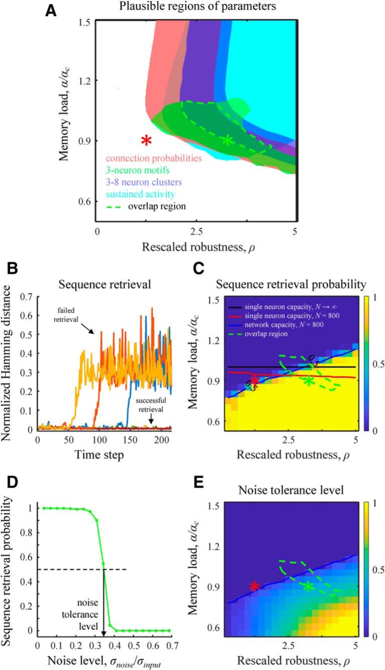
Values of rescaled robustness and memory load identified based on structural and dynamical properties of local cortical networks are consistent with the functional requirement of robust retrieval of stored memories. A, Region of parameters (dashed green line) that leads to a general agreement with the experimentally observed excitatory and inhibitory connection probabilities (red), excitatory 3-neuron motifs (green), 3–8 excitatory neuron clusters (blue), and sustained, irregular, asynchronous spiking activity (cyan). B, Retrieval of memory sequences in the absence of noise. The network is loaded with a memory sequence that it attempts to learn. The retrieval process is initialized at the start of the sequence, and deviations of subsequent network states from the loaded states are quantified with the Hamming distance normalized by the network size, N. The sequence is said to be successfully retrieved if the deviations are small. C, The success probability of sequence retrieval in the absence of noise as a function of rescaled robustness and relative memory load. The blue line, corresponding to the success probability of 0.5, defines the network capacity. Single-neuron critical capacity for N → ∞ (black line) and capacity for N = 800 (red line) are shown for reference. Dashed green contour is the overlap region from A. D, Probability of retrieving an entire memory sequence in the presence of postsynaptic noise. The network was configured at the green asterisk. Noise tolerance level is defined as the relative noise strength, σ_noise/σ_input, corresponding to the retrieval probability of 0.5. E, Map of noise tolerance level. In the identified parameter region, the network can tolerate noise that is comparable with the SD in postsynaptic input, σ_input.

This question was analyzed by using memories in the form single associative sequences (Fig. 1C), retrieval of which is more challenging compared with other memory formats due to propagation and accumulation of errors over the duration of memory playout. We first tested the retrieval of associative sequences in the absence of noise. For this, we initialized the network state at the beginning of the loaded sequence and monitored playout of the memory. The sequence is said to be retrieved successfully if the network states during the retrieval do not deviate substantially from the loaded states (Fig. 8B). In practice, there is no need to precisely define the threshold amount of deviation. This is because, for large networks, for example, N = 800, the Hamming distance between the loaded and retrieved sequences either remains within $\sim \sqrt{N}$ or diverges to ∼N. Figure 8C shows the probability of successful memory retrieval in the absence of noise as a function of rescaled robustness and relative memory load. The transition from successful memory retrieval to inability to retrieve the entire loaded sequence is relatively sharp, making it possible to define network capacity, analogously to the single-neuron capacity, as the sequence length for which the success rate in memory retrieval equals 0.5 (Fig. 8C, blue line). Network capacity can differ from single-neuron capacity, but this difference is expected to decrease with network size. Interestingly, the biologically plausible region of parameters overlaps with the single-neuron capacity curve, implying that individual neurons in the brain are loaded with associations close to their capacity. In addition, the biologically plausible region of parameters lies mostly below the network capacity curve, indicating that loaded memory sequences can be retrieved with high probability in the absence of noise.

To assess the degree of robustness of the memory retrieval process, we monitored memory playout in the presence of postsynaptic noise. In this experiment, random Gaussian noise of zero mean and SD σ_noise were added independently to all neurons at every step of the retrieval process. Network tolerance to noise is defined as σ_noise that results in the retrieval probability of 0.5, normalized by the baseline variations in postsynaptic input, σ_input (Fig. 8D). The latter represents the SD of postsynaptic input in the absence of noise (see Materials and Methods). The map of noise tolerance (Fig. 8E) shows that the biologically plausible region identified on the basis of structural and dynamical properties of cortical networks (Fig. 8E, green contour) has a non-zero overlap with the area in which memory retrieval is robust to noise. In this domain, the network can tolerate high noise-to-input ratios (up to 0.5), which serves as an independent validation of the associative model in terms of the hypothesized network function.

Effects of correlations on structure and dynamics of associative networks

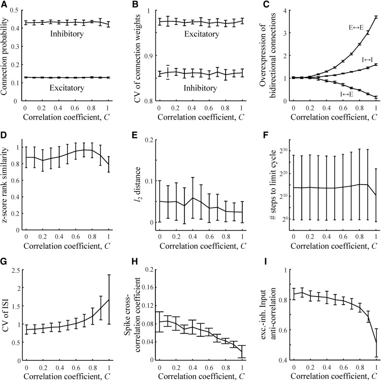
To assess the effects of correlations in associative memory states on the above described structural and dynamical network properties, we loaded the network, configured at the green asterisk of Figure 4, with memories in the form of associative pairs and varied the value of the correlation coefficient between the associative states, C, in the 0–1 range. At C = 0, the network is loaded with uncorrelated memory states, which is the case considered above; whereas at the other end of the range, C = 1, the network is loaded with memories in the form of point attractors. Figure 9A–E shows that, with the exception of overexpression of bidirectional 2-neuron motifs (Fig. 9C), structural network properties are not significantly affected by correlations. The overexpression ratio of bidirectionally connected excitatory pairs increases monotonically from 1 at C = 0 to ∼4 at C = 1 in agreement with values predicted in Brunel (2016) and the range of experimentally reported measurements. We also find that the overexpression ratio of bidirectionally connected inhibitory–excitatory pairs monotonically decreases with C, whereas this ratio for inhibitory–inhibitory pairs monotonically increases with C. Therefore, we predict that cortical systems with significant overexpression of bidirectionally connected excitatory–excitatory neuron pairs must have significant underexpression of inhibitory–excitatory connections. In such systems, inhibitory–inhibitory connections are slightly overexpressed, with the overexpression ratio not exceeding 1.6. Dynamical properties of associative memory networks can depend on correlations (Fig. 9F–I); but with the exception of very high C (C > 0.8), they remain consistent with the experimental measurements (Fig. 7, contours).

Figure 9.

Effects of correlations in associated network states on the structural and dynamical properties of model networks. A, Probabilities of inhibitory and excitatory connections in associative networks loaded with pairs of correlated network states (correlation coefficient C). The network is configured at the rescaled robustness and memory load defined by the green asterisk from Figure 4. Same for CVs of inhibitory and excitatory connection weights (B), overexpression ratios of excitatory–excitatory, inhibitory–excitatory, and inhibitory–inhibitory bidirectional connections (C), z score rank similarity for excitatory 3-neuron motifs 6, 7, 13, and 14 (D), l₂ distances between the logarithms of connection number probabilities in associative and cortical subnetworks of n = 6 neurons (E), number of steps to limit cycles (F), CV of ISI (G), cross-correlation coefficients of neuron spike trains (H), and anticorrelation coefficient of excitatory and inhibitory postsynaptic inputs to a neuron (I). Error bars in all panels indicate SDs calculated based on 100 networks.

Discussion

Our results suggest that local circuits of the mammalian brain operate in a high-weight regime in which individual neurons are loaded with associative memories close to their capacity (Fig. 8C) and the network can tolerate a relatively large amount of postsynaptic noise during memory retrieval. In this regime, many structural and dynamical properties of associative networks are in general agreement with the experimental measurements from various species and brain regions. It is important to point out that, due to large uncertainties in the reported measurements, we did not attempt to quantitatively fit the associative model to the data. The uncertainties originate from natural variability of network features across individuals, brain areas, and species, and are confounded by experimental biases and measurement errors. Instead, we rely on a large body of qualitative evidence to support our conclusions. This evidence includes the following: (1) sparse connectivity, with the probability of excitatory connections being lower than that for inhibitory connections; (2) distributions of non-zero connection weights with the CVs of excitatory and inhibitory weights being close to 1; (3) overexpression ratios in bidirectionally connected excitatory 2-neuron motifs; (4) overexpression of specific 3-neuron motifs; (5) distributions of connection numbers in subnetworks of 3–8 neurons showing clustering behavior; (6) sustained, irregular, and asynchronous firing activity with close to 1 CV of ISI and small positive cross-correlation in neuron activity; and (7) balance of EPSPs and IPSPs. Many of these features have been separately reported in various formulations of the associative model (Gardner and Derrida, 1988; Brunel et al., 2004; Chapeton et al., 2012, 2015; Brunel, 2016). Here, we show that, with a single set of model parameters, it is possible to account for these features collectively. In addition, the identified set of model parameters overlaps with the region in which loaded memories can be successfully recalled, even in the presence of postsynaptic noise (Fig. 8E), providing an independent functional validation of the theory.

We note that, in the absence of temporal correlations, C = 0, results of this study are independent of the format of associative memories (for examples, see Fig. 1C) which is not known and is likely to be area dependent. Therefore, this case provides a baseline for structural and dynamical properties in primary and association areas, which may use different memory formats. Correlations in memory states (C > 0) can, in general, affect the network properties, but as it is illustrated for one specific memory format in Figure 9, many of the described properties remain unaffected. A notable exception is that the overexpression of bidirectional connections increases with C. This effect was previously examined by Brunel (2016) for the extreme cases of storing uncorrelated patterns and point attractors. Here, we extended the analysis on temporal correlations of arbitrary strength and on multiple connection types. In particular, we predict that, if temporal correlations are responsible for the overexpression of bidirectional excitatory connections, then bidirectional inhibitory–excitatory connections must be greatly underexpressed (Fig. 9C).

The McCulloch and Pitts neuron model is often used in computational studies because of its simplicity, but is it biologically realistic enough for modeling associative learning in the brain? This question was explored in the work of Memmesheimer et al. (2014) who have shown that Leaky Integrate-and-Fire neurons, which are somewhat more realistic, can also be used to learn spike sequences, and the results of the two models are in good agreement so long as the firing probability is sufficiently low (e.g., f = 0.2). In addition, the methods of convex optimization were used in this study to load memories into networks. These methods are fast and accurate but are not biologically plausible. Thus, we developed a perceptron-type learning rule, Equations 3 and 4, that can match the accuracy of convex optimization (Fig. 1D) and can be used to reproduce the results of this study.

Although the considered model of an all-to-all potentially connected network of two generic neuron classes, inhibitory and excitatory, reproduces many experimentally observed network properties, this is an indisputably simplistic depiction of cortical networks. A more realistic model could be built by loading associative memories into a potentially connected network (e.g., a cortical column) constructed by putting together reconstructed morphologies of axonal and dendritic arbors of multiple neuron classes. Functional connectivity in such a network is constrained by neuron class-specific densities and morphologies, and it would be interesting to see whether these structural constraints are sufficient to give rise to the cell-type-dependent features of cortical connectivity and dynamics.

Because local cortical circuits function in the high-weight regime, Nwf >> h, the average excitatory and inhibitory postsynaptic inputs are significantly greater than the threshold of firing (Fig. 10). In the identified region of rescaled robustness and memory load (e.g., for the green asterisk of Fig. 4), these potentials in magnitude exceed the threshold of firing by factors of 6.3 and 7.8, respectively (Table 1). In this regime, excitatory and inhibitory potentials are strongly anticorrelated (Fig. 7D2), which is reminiscent of the balanced state described by many authors (Shu et al., 2003; Wehr and Zador, 2003; Haider et al., 2006; Okun and Lampl, 2008; Graupner and Reyes, 2013; Xue et al., 2014; Denève and Machens, 2016). We note, however, that there is a difference in how the balance of excitatory and inhibitory potentials is realized in the associative versus balanced networks. The difference originates from the scaling of synaptic weight with network size. In associative networks, synaptic weight is inversely proportional to N; whereas in balanced networks, inverse proportionality to $\sqrt{N}$ is assumed. In the former model, the average excitatory and inhibitory postsynaptic inputs to a neuron remain unchanged as the network size increases, and balance is the consequence of the high-weight regime; whereas in the latter model, balance emerges with increasing N as postsynaptic potentials diverge, which may be unsettling. On the other hand, Rubin et al. (2017) argue that, due to the above scaling difference, synaptic connections in the associative model are weaker, and the network is unstable to large, O(h), noise arising from processes within neurons (e.g., threshold fluctuations). We agree that the susceptibility of associative networks to this type of noise is a concern for infinitely large systems. However, there are no biological data on the scaling of noise with network size, and having O(h) noise may be unrealistic. More importantly, since local brain networks are finite, robustness to this type of noise can always be achieved by increasing w (i.e., in the high-weight regime). For example, an associative network of N = 800 neurons, configured at the green asterisk of Figure 4, can tolerate CVs in threshold fluctuations up to 1.1. Aside from the issue of robustness to O(h) noise, we show that, in the high-weight regime, results of the balanced and associative models become independent of scaling details and converge to the same solution (see Materials and Methods; Fig. 2). Therefore, associative learning in both models will lead to networks with identical structural and dynamical properties.

Figure 10.

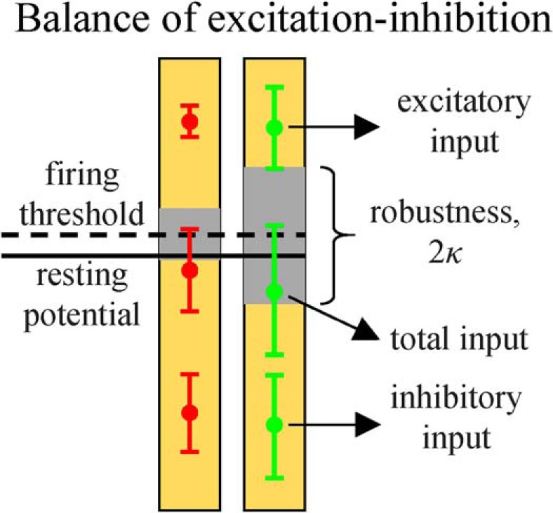
Excitatory and inhibitory inputs in relation to the firing threshold and robustness. Left and right halves of the figure are based on the data from Table 1 and correspond to the red and green asterisks from Figure 4. The average excitatory and inhibitory inputs are much larger than the threshold of firing. However, the total input lies within 1 SD from the firing threshold due to a partial cancellation of its excitatory and inhibitory components.

Table 1.

Input and output model parameters corresponding to the red and green asterisks of Figure 4

	Parameter name	Red asterisk	Green asterisk
Input parameters	Number of neurons, N	800	800
	Inhibitory neuron fraction, Ninh/N	0.20	0.20
	Firing probability, f	0.20	0.20
	Threshold of firing, h	20 mV	20 mV
	Scaled average absolute connection weight, Nwf /h	14	14
	Relative memory load, α/αc	0.90	0.90
	Rescaled robustness, ρ	1.25	3.25
Output parameters	Memory load, α	0.38	0.20
	Robustness parameter, κ	25 mV	64 mV
	Excitatory connection probability, Pexccon	0.26	0.14
	Inhibitory connection probability, Pinhcon	0.66	0.46
	CV of excitatory connection weights	0.89	0.99
	CV of inhibitory connection weights	0.75	0.86
	Average number of steps to limit cycle	32	2.3 × 104
	CV of ISI	0.67	0.88
	Spike cross-correlation coefficient	0.24	0.09
	EPSP (mean ± SD)	133 ± 14 mV	125 ± 38 mV
	IPSP (mean ± SD)	−144 ± 35 mV	−155 ± 48 mV
	Total postsynaptic potential (mean ± SD)	−11 ± 38 mV	−30 ± 60 mV
	Excitatory-inhibitory input correlation coefficient	−0.96	−0.79
	Sequence retrieval probability	0.08	1
	Noise tolerance, σnoise/σinput	0	0.35

References

- Altman A, Gondzio J (1999) Regularized symmetric indefinite systems in interior point methods for linear and quadratic optimization. Optimization Methods Soft 11:275–302. 10.1080/10556789908805754 [DOI] [Google Scholar]
- Amit DJ, Brunel N (1997) Model of global spontaneous activity and local structured activity during delay periods in the cerebral cortex. Cereb Cortex 7:237–252. 10.1093/cercor/7.3.237 [DOI] [PubMed] [Google Scholar]
- Bourne JN, Harris KM (2011) Coordination of size and number of excitatory and inhibitory synapses results in a balanced structural plasticity along mature hippocampal CA1 dendrites during LTP. Hippocampus 21:354–373. 10.1002/hipo.20768 [DOI] [PMC free article] [PubMed] [Google Scholar]
- Boyd SP, Vandenberghe L (2004) Convex optimization. Cambridge, UK: Cambridge UP. [Google Scholar]
- Brunel N. (2000) Dynamics of sparsely connected networks of excitatory and inhibitory spiking neurons. J Comput Neurosci 8:183–208. 10.1023/A:1008925309027 [DOI] [PubMed] [Google Scholar]
- Brunel N. (2016) Is cortical connectivity optimized for storing information? Nat Neurosci 19:749–755. 10.1038/nn.4286 [DOI] [PubMed] [Google Scholar]
- Brunel N, Hakim V, Isope P, Nadal JP, Barbour B (2004) Optimal information storage and the distribution of synaptic weights: perceptron versus Purkinje cell. Neuron 43:745–757. 10.1016/j.neuron.2004.08.023 [DOI] [PubMed] [Google Scholar]
- Buracas GT, Zador AM, DeWeese MR, Albright TD (1998) Efficient discrimination of temporal patterns by motion-sensitive neurons in primate visual cortex. Neuron 20:959–969. 10.1016/S0896-6273(00)80477-8 [DOI] [PubMed] [Google Scholar]
- Chapeton J, Fares T, LaSota D, Stepanyants A (2012) Efficient associative memory storage in cortical circuits of inhibitory and excitatory neurons. Proc Natl Acad Sci U S A 109:E3614–E3622. 10.1073/pnas.1211467109 [DOI] [PMC free article] [PubMed] [Google Scholar]
- Chapeton J, Gala R, Stepanyants A (2015) Effects of homeostatic constraints on associative memory storage and synaptic connectivity of cortical circuits. Front Comput Neurosci 9:74. 10.3389/fncom.2015.00074 [DOI] [PMC free article] [PubMed] [Google Scholar]
- Clopath C, Nadal JP, Brunel N (2012) Storage of correlated patterns in standard and bistable Purkinje cell models. PLoS Comput Biol 8:e1002448. 10.1371/journal.pcbi.1002448 [DOI] [PMC free article] [PubMed] [Google Scholar]
- Cohen MR, Kohn A (2011) Measuring and interpreting neuronal correlations. Nat Neurosci 14:811–819. 10.1038/nn.2842 [DOI] [PMC free article] [PubMed] [Google Scholar]
- Dale H. (1935) Pharmacology and nerve-endings. Proc R Soc Med 28:319–332. [DOI] [PMC free article] [PubMed] [Google Scholar]
- Denève S, Machens CK (2016) Efficient codes and balanced networks. Nat Neurosci 19:375–382. 10.1038/nn.4243 [DOI] [PubMed] [Google Scholar]
- Edwards SF, Anderson PW (1975) Theory of spin glasses. J Phys F Metal Phys 5:965–974. 10.1088/0305-4608/5/5/017 [DOI] [Google Scholar]
- El-Boustani S, Ip JP, Breton-Provencher V, Knott GW, Okuno H, Bito H, Sur M (2018) Locally coordinated synaptic plasticity of visual cortex neurons in vivo. Science 360:1349–1354. 10.1126/science.aao0862 [DOI] [PMC free article] [PubMed] [Google Scholar]
- Gal E, London M, Globerson A, Ramaswamy S, Reimann MW, Muller E, Markram H, Segev I (2017) Rich cell-type-specific network topology in neocortical microcircuitry. Nat Neurosci 20:1004–1013. 10.1038/nn.4576 [DOI] [PubMed] [Google Scholar]
- Gardner E, Derrida B (1988) Optimal storage properties of neural network models. J Phys A Math Gen 21:271–284. 10.1088/0305-4470/21/1/031 [DOI] [Google Scholar]
- Graupner M, Reyes AD (2013) Synaptic input correlations leading to membrane potential decorrelation of spontaneous activity in cortex. J Neurosci 33:15075–15085. 10.1523/JNEUROSCI.0347-13.2013 [DOI] [PMC free article] [PubMed] [Google Scholar]
- Haider B, Duque A, Hasenstaub AR, McCormick DA (2006) Neocortical network activity in vivo is generated through a dynamic balance of excitation and inhibition. J Neurosci 26:4535–4545. 10.1523/JNEUROSCI.5297-05.2006 [DOI] [PMC free article] [PubMed] [Google Scholar]
- Hastie T, Tibshirani R, Friedman JH (2009) The elements of statistical learning: data mining, inference, and prediction, Ed 2 New York: Springer. [Google Scholar]
- Holmgren C, Harkany T, Svennenfors B, Zilberter Y (2003) Pyramidal cell communication within local networks in layer 2/3 of rat neocortex. J Physiol 551:139–153. 10.1113/jphysiol.2003.044784 [DOI] [PMC free article] [PubMed] [Google Scholar]
- Holt GR, Softky WR, Koch C, Douglas RJ (1996) Comparison of discharge variability in vitro and in vivo in cat visual cortex neurons. J Neurophysiol 75:1806–1814. 10.1152/jn.1996.75.5.1806 [DOI] [PubMed] [Google Scholar]
- Holtmaat A, Wilbrecht L, Knott GW, Welker E, Svoboda K (2006) Experience-dependent and cell-type-specific spine growth in the neocortex. Nature 441:979–983. 10.1038/nature04783 [DOI] [PubMed] [Google Scholar]
- Hopfield JJ. (1982) Neural networks and physical systems with emergent collective computational abilities. Proc Natl Acad Sci U S A 79:2554–2558. 10.1073/pnas.79.8.2554 [DOI] [PMC free article] [PubMed] [Google Scholar]
- Kim SK, Nabekura J (2011) Rapid synaptic remodeling in the adult somatosensory cortex following peripheral nerve injury and its association with neuropathic pain. J Neurosci 31:5477–5482. 10.1523/JNEUROSCI.0328-11.2011 [DOI] [PMC free article] [PubMed] [Google Scholar]
- Lefort S, Tomm C, Floyd Sarria JC, Petersen CC (2009) The excitatory neuronal network of the C2 barrel column in mouse primary somatosensory cortex. Neuron 61:301–316. 10.1016/j.neuron.2008.12.020 [DOI] [PubMed] [Google Scholar]
- Markram H, Lübke J, Frotscher M, Roth A, Sakmann B (1997) Physiology and anatomy of synaptic connections between thick tufted pyramidal neurones in the developing rat neocortex. J Physiol 500:409–440. 10.1113/jphysiol.1997.sp022031 [DOI] [PMC free article] [PubMed] [Google Scholar]
- McCulloch W, Pitts W (1943) A logical calculus of the ideas immanent in nervous activity. Bull Math Biol 5:115–133. [PubMed] [Google Scholar]
- Memmesheimer RM, Rubin R, Olveczky BP, Sompolinsky H (2014) Learning precisely timed spikes. Neuron 82:925–938. 10.1016/j.neuron.2014.03.026 [DOI] [PubMed] [Google Scholar]
- Okun M, Lampl I (2008) Instantaneous correlation of excitation and inhibition during ongoing and sensory-evoked activities. Nat Neurosci 11:535–537. 10.1038/nn.2105 [DOI] [PubMed] [Google Scholar]
- Perin R, Berger TK, Markram H (2011) A synaptic organizing principle for cortical neuronal groups. Proc Natl Acad Sci U S A 108:5419–5424. 10.1073/pnas.1016051108 [DOI] [PMC free article] [PubMed] [Google Scholar]
- Renart A, de la Rocha J, Bartho P, Hollender L, Parga N, Reyes A, Harris KD (2010) The asynchronous state in cortical circuits. Science 327:587–590. 10.1126/science.1179850 [DOI] [PMC free article] [PubMed] [Google Scholar]
- Rieubland S, Roth A, Häusser M (2014) Structured connectivity in cerebellar inhibitory networks. Neuron 81:913–929. 10.1016/j.neuron.2013.12.029 [DOI] [PMC free article] [PubMed] [Google Scholar]
- Rosenblatt F. (1962) Principles of neurodynamics: perceptrons and the theory of brain mechanisms. Washington, DC: Spartan. [Google Scholar]
- Rubin R, Abbott LF, Sompolinsky H (2017) Balanced excitation and inhibition are required for high-capacity, noise-robust neuronal selectivity. Proc Natl Acad Sci U S A 114:E9366–E9375. 10.1073/pnas.1705841114 [DOI] [PMC free article] [PubMed] [Google Scholar]
- Rubinov M, Sporns O (2010) Complex network measures of brain connectivity: uses and interpretations. Neuroimage 52:1059–1069. 10.1016/j.neuroimage.2009.10.003 [DOI] [PubMed] [Google Scholar]
- Shadlen MN, Newsome WT (1998) The variable discharge of cortical neurons: implications for connectivity, computation, and information coding. J Neurosci 18:3870–3896. 10.1523/JNEUROSCI.18-10-03870.1998 [DOI] [PMC free article] [PubMed] [Google Scholar]
- Sherrington D, Kirkpatrick S (1975) Solvable model of a spin glass. Phys Rev Lett 35:1792–1796. 10.1103/PhysRevLett.35.1792 [DOI] [Google Scholar]
- Shu Y, Hasenstaub A, McCormick DA (2003) Turning on and off recurrent balanced cortical activity. Nature 423:288–293. 10.1038/nature01616 [DOI] [PubMed] [Google Scholar]
- Softky WR, Koch C (1993) The highly irregular firing of cortical cells is inconsistent with temporal integration of random EPSPs. J Neurosci 13:334–350. 10.1523/JNEUROSCI.13-01-00334.1993 [DOI] [PMC free article] [PubMed] [Google Scholar]
- Song S, Sjöström PJ, Reigl M, Nelson S, Chklovskii DB (2005) Highly nonrandom features of synaptic connectivity in local cortical circuits. PLoS Biol 3:e68. 10.1371/journal.pbio.0030068 [DOI] [PMC free article] [PubMed] [Google Scholar]
- Spitzer NC. (2017) Neurotransmitter switching in the developing and adult brain. Annu Rev Neurosci 40:1–19. 10.1146/annurev-neuro-072116-031204 [DOI] [PubMed] [Google Scholar]
- Stepanyants A, Chklovskii DB (2005) Neurogeometry and potential synaptic connectivity. Trends Neurosci 28:387–394. 10.1016/j.tins.2005.05.006 [DOI] [PubMed] [Google Scholar]
- Stepanyants A, Hirsch JA, Martinez LM, Kisvárday ZF, Ferecskó AS, Chklovskii DB (2008) Local potential connectivity in cat primary visual cortex. Cereb Cortex 18:13–28. 10.1093/cercor/bhm027 [DOI] [PubMed] [Google Scholar]
- Stevens CF, Zador AM (1998) Input synchrony and the irregular firing of cortical neurons. Nat Neurosci 1:210–217. 10.1038/659 [DOI] [PubMed] [Google Scholar]
- Tibshirani R. (1996) Regression shrinkage and selection via the lasso. J R Statist Soc B 58:267–288. [Google Scholar]
- van Vreeswijk C, Sompolinsky H (1996) Chaos in neuronal networks with balanced excitatory and inhibitory activity. Science 274:1724–1726. 10.1126/science.274.5293.1724 [DOI] [PubMed] [Google Scholar]
- van Vreeswijk C, Sompolinsky H (1998) Chaotic balanced state in a model of cortical circuits. Neural Comput 10:1321–1371. 10.1162/089976698300017214 [DOI] [PubMed] [Google Scholar]
- Vegué M, Perin R, Roxin A (2017) On the structure of cortical microcircuits inferred from small sample sizes. J Neurosci 37:8498–8510. 10.1523/JNEUROSCI.0984-17.2017 [DOI] [PMC free article] [PubMed] [Google Scholar]
- Wang Y, Markram H, Goodman PH, Berger TK, Ma J, Goldman-Rakic PS (2006) Heterogeneity in the pyramidal network of the medial prefrontal cortex. Nat Neurosci 9:534–542. 10.1038/nn1670 [DOI] [PubMed] [Google Scholar]
- Wehr M, Zador AM (2003) Balanced inhibition underlies tuning and sharpens spike timing in auditory cortex. Nature 426:442–446. 10.1038/nature02116 [DOI] [PubMed] [Google Scholar]
- Xue M, Atallah BV, Scanziani M (2014) Equalizing excitation-inhibition ratios across visual cortical neurons. Nature 511:596–600. 10.1038/nature13321 [DOI] [PMC free article] [PubMed] [Google Scholar]
- Zhang D, Zhang C, Stepanyants A (2018) Robust associative learning is sufficient to explain structural and dynamical properties of local cortical circuits. bioRxiv. Advance online publication. Retrieved May 11, 2018. doi: 10.1101/320432. [DOI] [PMC free article] [PubMed] [Google Scholar]
Associated Data
This section collects any data citations, data availability statements, or supplementary materials included in this article.
Supplementary Materials