Mathematical models of hierarchically structured cell populations under equilibrium with application to the epidermis

Abstract

Abstract. There are three categories of keratinocytes in the germinative compartment of the epidermis – stem, transit‐amplifying and post‐mitotic. Their population structure is hierarchical. This means that stem cells differentiate into transit‐amplifying cells which, after a few rounds of division, become post‐mitotic cells. The cell processes of birth, differentiation, death and migration affect the composition and proliferation rate of the germinative compartment. These phenomena are quantified by various cell kinetic parameters. In this paper we derive equations that relate these parameters for different models of hierarchically structured cell populations in equilibrium. We include in the models asymmetric and symmetric division, variations in cell‐cycle times, apoptosis and variation in the number of transit generations. We conclude that variation in cell‐cycle times need only be considered if apoptosis is not negligible. If it is negligible, then only average cell‐cycle times are needed. Unfortunately, it is impossible to predict the importance of apoptosis from the available experimental data. However, the strength of its effect is determined by the other parameters, especially the fraction of cycling stem cells. We show that variation in the number of transit generations can have a potentially large effect on cell birth rate. We also show that cell birth rate does not directly depend on the mean transit‐amplifying cell‐cycle time, only on the mean stem cell‐cycle time. We argue that ‘homogeneous cell population’ equations should not be used to study hierarchical cell populations as has been done in the past. Finally we argue that stem cell parameters and transit‐amplifying cell parameters should not be lumped together.

INTRODUCTION

Keratinocytes constitute over 80% of the cells of the interfollicular epidermis (Holbrook 1994). They are shed at the skin surface and are replaced by division in the bottom‐most layer or layers, known as the germinative compartment. There is strong evidence for several types of keratinocytes in the germinative compartment, both in the mouse (Potten 1974, 1976; Potten et al. 1982; Clausen et al. 1986; Potten & Loeffler 1987; , Loeffler et al. 1987) and in the human (Dover & Potten 1983; Barrandon & Green 1985; Jensen et al. 1985; Leigh et al. 1985; Albers et al. 1986; Barrandon & Green 1987; Dover & Potten 1988; Watt 1988; Laporte & Heenen 1994; Jensen et al. 1999).

The cell types are categorized as stem, transit‐amplifying and post‐mitotic. Stem cells can divide indefinitely (Potten & Loeffler 1990), and are the source of interfollicular keratinocytes in normal epidermis. A stem cell can be in a resting state – known as the G₀ phase – or a proliferative state. Given an appropriate signal, stem cells differentiate into transit‐amplifying cells. These cells are in the first stages of terminal differentiation: the process in which cells lose the ability to divide, migrate from the germinative compartment, slowly fill with keratin and lose their nuclei and finally desquamate at the skin surface. Transit‐amplifying cells are thought to divide about three to five times. Once they stop dividing they are categorized as post‐mitotic.

Thus, the cells in the germinative compartment are heterogeneous in type and have a hierarchical population structure as shown in Fig. 1. Before the work of Potten (1974) it was assumed that all cells were stem cells and, therefore, homogeneous in type (Dover & Wright 1991).

Figure 1.

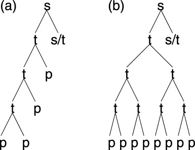
Proposed hierarchical population structures for the germinative compartment of the epidermis. On average, each stem cell division produces another stem cell (s) and a transit‐amplifying cell (t). Transit‐amplifying cells can either undergo asymmetric (a) or symmetric (b) division for a limited number of divisions. Transit‐amplifying cells finally become post‐mitotic cells (p) that migrate from the germinative compartment.

After a cell divides, if the daughter cells are of the same type, then a symmetric division has occurred. If the daughter cells are of different types then an asymmetric division has occurred. For example, a stem cell division that gives two stem cells or two transit‐amplifying cells is a symmetric division. A stem cell division that gives one stem cell and one transit‐amplifying cell is an asymmetric division. For stem cells this distinction is not important when the epidermis is in equilibrium. This is because each stem cell division must give, on average, one stem cell and one transit‐amplifying cell. If this was not the case, the density of stem cells would change with time, breaking our assumption of equilibrium. The distinction is important, however, for transit‐amplifying cell division. For asymmetric division, the density of post‐mitotic cells arising from the differentiation of a stem cell increases linearly with the number of transit generations (Fig. 1a). For symmetric division the increase is exponential (Fig. 1b).

The cell processes of birth, differentiation and death affects the composition and proliferation rate of the germinative compartment. In this paper we are interested in these effects in a hierarchical population of cells. We want to derive analytical equations that relate various cell processes when the germinative compartment is in equilibrium. Surprisingly, this has not been done before even though hierarchical cell populations have been known about for some time. Many authors still apply ‘homogeneous cell population’ equations to hierarchical cell populations. It is not clear if this is a valid practice. It is at least questionable and we hope to provide some answers in this paper. As well as analytical equations, numerical analyses of various models of the germinative compartment are also possible: especially when the mathematics becomes intractable. Such work has been done by Potten et al. (1982) and Loeffler et al. (1987). Fitting of their numerical simulations to experimental data has provided strong evidence for a hierarchical population structure. We do not consider numerical simulations in this paper, except to validate our equations.

As well as deriving equations for asymmetric and symmetric division, we also consider variation in stem and transit‐amplifying cell‐cycle times, a stem‐cell G ₀‐phase, apoptosis and variations in the number of transit generations. Many other phenomena could be included, for example circadian rhythms, but these make the mathematics intractable.

We begin with the simplest case – asymmetric division, variation in cell‐cycle times, no apoptosis and no variation in transit generations – and progressively increase the complexity of the models. Fortunately, the method used to derive the equations remains the same even when the models become more complex.

The method proceeds as follows. We first derive the age distribution of the stem cells. Mathematically, this is written as s(a)δa (All notation is listed in Table 1). We assume newly born cells have an age a = 0. The term s(a) is known as a density function, and has the dimensions of cells per unit area of skin surface per unit age. When it is multiplied by a small interval of age δa (for example 1 h), it tells us the number of stem cells per unit area of skin surface between the ages of a and a+ δa. Here, age is defined as chronological age, that is, it advances at the same rate as time. (Sometimes, age is defined as the degree of maturity: as cells mature they age, but the rate of maturation may vary with time, when cells are fully mature they divide. This definition implies that all cells divide at the same age. However, cells can mature at different rates causing their cell‐cycle times to vary.) We treat age as a real number and not as an integer because it simplifies the mathematics. From the stem cell age distribution we can derive the rate stem cells differentiate into transit‐amplifying cells. A newly differentiated stem cell creates a first‐generation transit‐amplifying cell with an age a = 0. The differentiation rate of stem cells equals, by definition, the birth rate of first‐generation transit‐amplifying cells, and from the birth rate we can calculate the age distribution of first‐generation transit‐amplifying cells, t ₁(a)δa. We then iterate this method for subsequent transit‐amplifying cell generations: birth rate gives age distribution gives differentiation rate gives birth rate, and so on. Finally, having derived the age distributions for all transit‐amplifying cell generations, we can derive the total density of transit‐amplifying cells and the birth rate of post‐mitotic cells.

Table 1.

Definitions of cell kinetic parameters used in this paper

Stem cells
s ( a )	Density function of cycling stem cells
s ( a )δ a	Age distribution of cycling stem cells
s (0)	Rate of entry into stem cell‐cycle
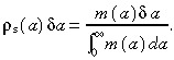
ρs(a)δa	Probability distribution of stem cell‐cycle times
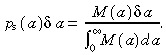
p s ( a )δ a	Apoptosis‐corrected probability distribution of stem cell‐cycle times
m ( a )δ a	Distribution of stem cell‐cycle times
M ( a )δ a	Apoptosis‐corrected distribution of stem cell‐cycle times
T̄s	Mean stem cell‐cycle time
T̂s	Effective stem cell‐cycle time
	Variance of stem cell‐cycle time
φs	Coefficient of variation of stem cell‐cycle time, σs/T̄s
N s	Density of stem cells
f	Fraction of cycling stem cells
r s	Rate of stem cell division
βs	Stem cell apoptotic rate
α	Stem cell apoptosis correction term
Transit‐amplifying cells
t i ( a )	Density function of ith generation transit‐amplifying cells
t i ( a )δ a	Age distribution of ith generation transit‐amplifying cells
t i (0)	Rate of entry into ith generation cell‐cycle
ρt(a)δa	Probability distribution of transit‐amplifying cell‐cycle times
p t ( a )δ a	Apoptosis‐corrected probability distribution of transit‐amplifying cell‐cycle times
T̄t	Mean transit‐amplifying cell‐cycle time
T̂s	Effective transit‐amplifying cell‐cycle time
	Variance of transit‐amplifying cell‐cycle time
φt	Coefficient of variation of transit‐amplifying cell‐cycle time, σt/T̄t
φt	Density of ith generation transit‐amplifying cells
N t	Density of all transit‐amplifying cells
g	Maximum number of transit‐amplifying cell generations
βt	Transit‐amplifying cell apoptotic rate
Q i	Probability of an ith generation transit‐amplifying cell giving two post‐mitotic cells
Pi
l A–D	Frequency of transit lineages
General
a	Chronological age of cells
δa	Small amount of age
r	Birth rate of post‐mitotic cells per unit area of skin surface
N	Total cell density in germinative compartment
r ′	Cell birth rate of germinative compartment
GF	Growth fraction of germinative compartment
ζ, ξ	Dummy variables

In order to derive analytical equations, we make the following assumptions which are further discussed in the conclusion. The epidermis is in equilibrium, that is, there are no changes in cell densities. Differentiation of stem cells to transit‐amplifying cells occurs immediately after stem cell division. All proliferating stem cells are desynchronized in their cell‐cycle. There are no circadian rhythms. The cell‐cycle times of daughter cells are not correlated. There is no correlation between transit‐amplifying cell‐cycle times and the number of rounds of division. Once a cell enters the cell‐cycle it always proceeds to division. Apoptosis occurs in both cell types, including cells in G ₀, and at the same rate throughout the cell‐cycle.

The equations we derive should be applicable to any hierarchically structured population of cells in equilibrium. Here, however, we apply them to mouse and human epidermis. We look at the effect of apoptosis in normal and psoriatic skin and the effect of variation in the number of transit generations. We highlight an interesting result on cell birth rate and look at possible ranges of various parameters based on published data. Finally we discuss the relationship between growth fraction, cell birth rate and cell‐cycle time.

MODELS OF HIERARCHICALLY STRUCTURED CELL POPULATIONS

The basic model

Stem cells The basic model includes a G ₀ phase for stem cells and variation in the cell‐cycle times of stem and transit‐amplifying cells. There is good evidence of variation in cell‐cycle times, and it may even be large (Duffill et al. 1976; Dover & Potten 1988). From these assumptions we will derive the age distribution of stem cells and their rate of differentiation into transit‐amplifying cells.

Note that we do not make the common assumption that the age distribution is rectangular or exponential – the age distribution is derived from the distribution of cell‐cycle times. Moreover, we are considering the age distribution of all stem cells irrespective of where they reside in the epidermis. This is different to Appleton et al. (1977) who considered age distributions in specific layers of the epidermis with a homogeneous cell population.

Consider a hierarchical structure for the germinative compartment. Let N _s be the number of stem cells per unit area of skin surface. A fraction f of stem cells are cycling, the rest, 1 − f, are in G ₀ phase. Let the probability distribution of stem cell‐cycle times be ρ_s(a) δa, where a is chronological age. The term ρ_s(a) is the probability density function of stem cell‐cycle times, and ρ_s(a)δa is the probability of a stem cell dividing between the ages of a and a + δa.

Let s(a)δa be the age distribution of stem cells. The dimension of s(a) is the number of stem cells per unit area of skin surface per unit age. Cells enter the cell‐cycle with age a = 0 either from the G ₀ compartment or immediately after dividing. Therefore the rate stem cells enter the cell‐cycle is s(0): for example, 5 cells per mm² per h.

To derive s(a) we write an equation for s(a + δa), let δa → 0 to get a differential equation, and then solve this equation. This is done as follows. The density of cells between ages a + δa and a + 2δa (s(a + δa)δa) equals the density of cells between ages a and a + δa (s(a)δa) that have aged by an amount δa, minus the density of cells with ages between a and a + δa that have divided in time δa (s(0)ρ_s(a)δa ²). Thus

s ( a  + δ a )δ a  =  s ( a )δ a  −  s (0)ρ _s ( a ) δ a² . (1)

Dividing through by δa ² and letting δa → 0 we get the differential equation

(2)

Solving gives

(3)

where ζ is a dummy variable. We multiply both sides of equation 3 by a small arbitrary age δa to find the age distribution of stem cells

(4)

This equation is interpreted as follows. When a = 0, cells have just entered the cell‐cycle and none have divided. Thus the integral equals zero and s(a)δa = s(0)δa. As cells age they can divide, the integral increases monotonically and hence the density of cells with age a declines with a. As a → ∞ the integral tends to one – because ρ_s is a probability density function – and the density of very old cells tends to zero.

We still need to determine the unknown s(0). This is found as follows. By definition, the total number of cycling stem cells per unit area of skin surface is fN _s. Thus:

(5)

Substituting in equation 3 and solving for s(0) we find

(6)

where we have defined

(7)

where ζ and ξ are dummy variables. In Appendix A we prove, for this case, that T̂_s is just the mean stem cell‐cycle time T̄_s Thus

(8)

(Note that we use ‘T _s’ to represent stem cell‐cycle time and not the usual S‐phase duration.) We will show later that this simplification does not hold when apoptosis occurs. In Fig. 2 we plot an example density function where the cell‐cycle times have a gamma distribution with a mean of 16 h and a standard deviation of 4 h (Dover & Potten 1988).

Figure 2.

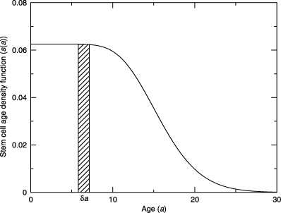
An example density function of stem cell age ( s ( a ), equation 3) . The cell‐cycle times are gamma distributed with a mean of 16 h and a standard deviation of 4 h. The stem cell age distribution ( s ( a )δ a ) is the density of cells with ages between a and a  + δ a , where δ a is a small amount of age. The area under the curve gives the density of cycling stem cells f / N _s , which in this case has been normalized to one.

In conclusion, we have derived the stem cell age distribution in terms of f, N _s and ρ_s. To calculate the age distribution of first‐generation transit‐amplifying cells, we need to know the rate at which stem cells divide. Let us denote this by r _s. In equilibrium and without cell loss, the rate of division of stem cells must equal their rate of entry into the cell‐cycle, therefore r _s = s(0). So

(9)

First‐generation transit‐amplifying cells Let the age distribution of first‐generation transit‐amplifying cells be t ₁(a)δa. In equilibrium, a stem cell division produces, on average, one stem cell and one transit‐amplifying cell. Therefore the birth rate of first‐generation transit‐amplifying cells (t ₁(0)) equals the division rate of stem cells (r _s). So t ₁(0) = fN _s/T̄_s. Let (a)δa be the probability distribution of first‐generation transit‐amplifying cell‐cycle times. Using the same arguments as for stem cells, it is easy to show that t ₁(a)δa is given by

(10)

This equation has a similar interpretation as equation 3.

Let be the density of first‐generation transit‐amplifying cells. By definition it is given by

(11)

substituting in equation 10 gives

(12)

where is the mean cell‐cycle time of first‐generation transit‐amplifying cells. So the density of first‐generation transit‐amplifying cells equals the rate at which they are born times their mean cell‐cycle time.

We must now consider asymmetric and symmetric division separately.

Asymmetric division Without apoptosis, the rate of division of first‐generation transit‐amplifying cells equals their rate of birth, t ₁(0). On division, these cells give rise to one post‐mitotic cell and one second‐generation transit‐amplifying cell. Therefore, the birth rate of second‐generation cells (t ₂(0)) equals t ₁(0). This argument applies in general to all transit generations, hence t _i+1(0) = t _i(0) = t ₁(0). Thus

(13)

Generalizing and combining (10), (11) we see that for ith generation cells

(14)

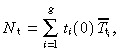
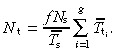
If there are g generations of transit‐amplifying cells then the density of all transit‐amplifying cells, N _t, is

(15)

(16)

(17)

If all transit‐amplifying cell generations have the same mean cell‐cycle time ( for i = 1, … , g), then equation 17 becomes

(18)

So the density of transit‐amplifying cells for asymmetric division is proportional to the density of cycling stem cells, the number of transit generations and the mean cell‐cycle time of transit‐amplifying cells, and it is inversely proportional to the mean cell‐cycle time of stem cells.

Now we want to calculate the rate at which post‐mitotic cells are born: let us denote this by r. This has dimensions of cells per unit area of skin surface per unit time. It is derived as follows. The rate ith generation transit‐amplifying cells produce daughters is 2t _i(0) (twice their birth rate). The birth rate of i + 1 generation cells is t _i+1(0), by definition. Hence the birth rate of post‐mitotic cells from ith generation transit‐amplifying cells is 2t _i(0) −t _i+1(0). Therefore, the total birth rate of post‐mitotic cells per unit area of skin surface is

(19)

There are no g + 1 generation cells so t _g+1(0) = 0. We substitute in equation 13 and do some simple manipulation to give

(20)

Notice that this equation is independent of the mean transit‐amplifying cell‐cycle time. See Cell birth rate section for a discussion of this important point. The parameter r tells us how many cells per unit are of skin surface leave the germinative compartment per unit time. If there is no cell loss in the upper layers of the epidermis, it also equals the desquamation rate per unit area of skin surface.

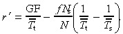
A commonly used kinetic parameter is the cell birth rate. This has dimensions of inverse time, or often cells per 1000 cells per unit time. Let us denote the cell birth rate by r′. It is related to the cell birth rate per unit area of skin surface by the following equation

(21)

where N is the number of cells per unit area of skin surface in the germinative compartment. Another useful parameter is the growth fraction. This is defined as the fraction of actively cycling cells in the germinative compartment, that is,

(22)

Later, we will derive a general equation that relates these two parameters in a hierarchically structured population (see Growth fraction, birth rate and cell‐cycle time section).

Symmetric division For symmetric division, the birth rate of i + 1 generation transit‐amplifying cells is twice the rate of division of ith generation cells

t_{i +1} (0) = 2 t_i (0). (23)

Solving this difference equation and substituting in equation 13 gives

(24)

The total density of transit‐amplifying cells is given by equation 16, therefore

(25)

If all transit‐amplifying cell generations have the same mean cell‐cycle time (), then equation 25 becomes

(26)

The post‐mitotic cell birth rate per unit area of skin surface is

r  = 2 t_g (0), (27)

from equation 24 this gives

(28)

which again is independent of mean transit‐amplifying cell‐cycle time.

The difference between asymmetric and symmetric division is that N _t and r increase linearly and exponentially, respectively, with the number of transit‐amplifying generations as expected from Fig. 1.

The basic model with apoptosis

Stem cells

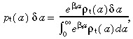
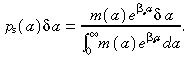
We now consider the effects of apoptosis on transit‐amplifying cell density and cell birth rate per unit area of skin surface. We assume that apoptosis occurs in both stem and transit‐amplifying cells. Firstly, the stem cells. From experiments we would measure the probability distribution of stem cell‐cycle times, ρ_s(a)δa. However, apoptosis modifies this distribution by killing cells before they divide. If there was no apoptosis, we would expect to see more cells dividing at later ages. If p _s(a)δa is the probability distribution of stem cell‐cycle times without apoptosis, then these two probability distributions are related by the equation

(29)

where β_s is the rate of stem cell apoptosis. See Appendix B for the derivation of this equation. This equation is based on the assumption that the probability of cell death is constant throughout the cell‐cycle. There is no evidence for this assumption, but it is the simplest. If the rate varies during the cell‐cycle, the mathematical models would become more complex.

Knowing p _s(a)δa allows us to calculate the age distribution of the stem cells. We again write an equation for s(a + δa) and let δa → 0. The density of cells between ages a + δa and a + 2δa (s(a + δa)δa) equals the density of cells between ages a and a + δa that have aged by an amount δa (s(a)δa) minus, the density of cells between ages a and a + δa that have divided in time , minus the density of cells between ages a and a + δa that have been lost due to apoptosis in time δa (β_s s(a)δa ²). Thus

(30)

The term comprises two factors. The first, s(0)p _s(a)δa ², is the density of cells that would have divided between ages a and a + δa in time δa if there was no apoptosis. This isthe same as in equation 1. The second, is a correction factor to account for those cells thatwould have divided between ages a and a + δa in time δa but have been lost due to apoptosis.

Dividing through by δa ² and letting δa → 0 we get the differential equation

(31)

Solving, we get the age distribution of the stem cells:

(32)

If there is no apoptosis then β _s = 0, and we recover equation 3. The interpretation of this equation is similar to that of equation 3. However, the density of cells between ages a and a + δa declines with age, not only because of cell division but also because of apoptosis.

As before thus s(0) is given by

(33)

where T̂_s is an effective stem cell‐cycle time due to the combined effects of apoptosis and variation in cell‐cycle time. It is given by

(34)

where ζ and ξ are dummy variables. We show in Appendix C that this integral can be simplified to

(35)

By comparing (7), (34) we can see that T̂_s ≤ T̄_s, and that if β_s = 0, T̂_sT̄_s. If we want to use the observed cell‐cycle time distribution ρ_s(a)δa instead of p _s(a)δa, we can substitute in equation 29 to get

(36)

As an example, if the observed probability distribution of stem cell‐cycle times ρ_s(a)δa, has a gamma distribution (Dover & Potten 1988) then

(37)

where φ_s = σ_s/T̄_s is the coefficient of variation of stem cell‐cycle times.

We now need to calculate the rate of stem cell division r _s. In equilibrium the rate stem cells enter the cell‐cycle must equal the rate they leave. Without apoptosis, this implied that the rate stem cells enter the cell‐cycle equalled the rate of stem cell division. With apoptosis, however, we must include the rate of death of cycling stem cells. Therefore,

s (0) =  β_sfN_s  +  r_s , (38)

where the first term on the right‐hand side reflects loss of cycling cells due to apoptosis and the second term is the rate of cell division. Substituting in equation 33 and re‐arranging we find

(39)

Notice that if β_sT̂_s > 1 then r _s is negative, implying that, on average, stem cells die before they can divide – causing local loss of epidermis.

First‐generation transit‐amplifying cells We now need to find the birth rate of first‐generation transit‐amplifying cells, by definition, t ₁(0). When stem cells divide, a proportion remain stem cells in order to maintain their density: the remainder differentiate into transit‐amplifying cells. Without apoptosis, the ratio of stem to transit‐amplifying daughters is 1 : 1. With apoptosis both resting and cycling stem cells need to be replenished. Stem cells are lost at a rate r _s + β_s N _s. The first term reflects loss due to stem cell division, the second term loss due to apoptosis. To maintain stem cell density, the rate of gain (from division) must equal the rate of loss. Because new cells are born at a rate 2r _s, the rate of entry into the transit compartment is, therefore, t ₁(0) = 2r _s − (r _s + β_s N _s) = r _s − β_s N _s. For mathematical convenience let us introduce the parameter α such that

(40)

We can find α by using equation 39:

(41)

As apoptosis becomes negligible α → 1.

In a similar fashion to the stem cells, we define two probability distributions of transit‐amplifying cell‐cycle times. Let ρ_t(a) δa be the experimentally observed distribution and let p _t(a) δa be the corrected distribution that removes the effect of apoptosis. The relationship between them is

(42)

where β_t is the rate of transit‐amplifying cell apoptosis. We will assume that all transit‐amplifying cell generations have the same rate of apoptosis and cell‐cycle time probability distribution. This is for mathematical convenience. The assumption can be dropped with no major changes in our conclusions.

As before, we need to derive the age distribution of first‐generation transit‐amplifying cells t ₁(a) δa, which satisfies

(43)

Taking δa → 0 and solving the differential equation gives

(44)

The density of first‐generation transit‐amplifying cells, is given by Thus

(45)

(46)

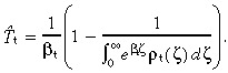
where T̂_t is the effective transit‐amplifying cell‐cycle time, with similar properties to T̂_s. It is given by

(47)

or, using the observed probability distribution of transit‐amplifying cell‐cycle times,

(48)

Again, we have to consider asymmetric and symmetric division separately.

Asymmetric division For asymmetric division, the birth rate of i + 1 generation transit‐amplifying cells (t _i+1(0)) equals the division rate of ith generation cells. This, in turn, equals the birth rate of ith generation cells minus their apoptotic rate. Therefore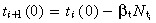. The general form of equation 14 is

(49)

Substitution of equation 49 into t _i+1(0) gives

(50)

Hence, the birth rate of i + 1 generation cells is smaller, by a factor of 1 − β_tT̂_t than ith generation cells. Solving and substituting in equation 40 gives

(51)

The total density of transit‐amplifying cells is given by

(52)

We use equation 49 to get

(53)

Substituting in equation 51 gives

(54)

When β_s and β_t equal zero this equation reduces to equation 18, that is, α = 1, T̂_s = T̄_s and T̂_t = T̄_t.

Now for the birth rate of post‐mitotic cells. The rate ith generation transit‐amplifying cells produce daughters is 2t_i(0)(1 − β_tT̂_t). The birth rate of i + 1 generation cells is t _i+1(0). Hence the birth rate of post‐mitotic cells from ith generation transit‐amplifying cells is 2t_i(0)(1 − β_tT̂_t) −t _i+1 Therefore, the total birth rate of post‐mitotic cells per unit area of skin surface is

(55)

where t _g+1(0) = 0. Substituting in equation 51 gives

(56)

Comparison with the case without apoptosis (equation 20), we observe several differences. The whole equation is multiplied by the factor α, thus stem‐cell apoptosis reduces cell birth rate. We must now use the effective cell‐cycle times instead of average times. The birth rate now depends on transit‐amplifying cell‐cycle times, albeit through the small term β_tT̂_t. This term affects the number of transit generations g.

Symmetric division For symmetric division, i + 1 generation cells are born at a rate Using equation 49 this gives t_i+1(0) = 2t_i(0)(1 − β_tT̂_t Solving andsubstituting into equation 53 gives

(57)

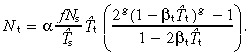
Post‐mitotic cells are born at a rate per unit area of skin surface of 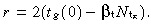Using equation 49 gives r = 2t_g(0)(1 − β_tT̂_t). Using equation 51 gives

(58)

The basic model with apoptosis and variation in the number of transit generations

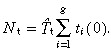
Measuring transit‐amplifying cell lineages So far, we have assumed that every transit‐amplifying cell lineage derived from a stem‐cell division has the same number of generations. We have also assumed, for symmetric division, that the daughters of every transit‐amplifying cell of a given generation are of the same type – either transit or post‐mitotic cells. We now drop these assumptions. To proceed, we need to know the probability, Q_i, that an ith generation transit‐amplifying cell produces two post‐mitotic cells. Experimentally, Q _i can be measured directly if we can determine which generation a dividing transit‐amplifying cell is in, or indirectly by measuring the frequency of each transit‐amplifying cell lineage. Fig. 3 shows an example of the indirect method. If there is a maximum of three transit generations then there are three possible asymmetric lineages and four symmetric lineages. The values of Q _i are calculated from the frequencies of the lineages. Let g be the maximum number of transit generations. Then Q _g must equal one and Q _i, for i < g, can take any value from zero up to, but not including, one. If apoptosis occurs in a lineage it may not be possible to assign it to a specific class. Therefore, these lineages should be discounted.

Figure 3.

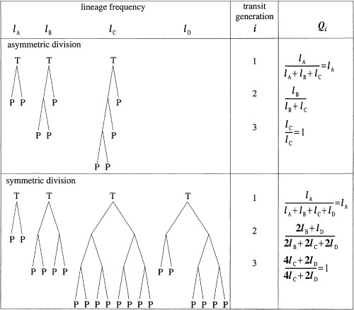
An example showing the calculation of Q _i from the frequencies of all possible transit‐amplifying cell lineages for asymmetric and symmetric division and g  = 3. Note that l _A  +  l _B  +  l _C  = 1 and l _A  +  l _B  +  l _C  +  l _D  = 1 for asymmetric and symmetric division, respectively. Q _i is calculated by summing, over all lineages, those i th generation cells that give rise to two post‐mitotic cells and dividing by the total number of i th generation cells.

Asymmetric division

As before, we need to find the birth rate per unit area of skin surface of ith generation cells (t_i(0)). This proceeds as follows. The rate of division of ith generation cells is equal to the rate of birth of ith generation cells (t_i(0)), minus the rate of apoptosis . Using equation 49, the division rate is t_i(0)(1 − β_tT̂_t). A fraction Q_i, of ith generation cells divide into two post‐mitotic cells. The rest, 1 − Q_i, divide into one post‐mitotic cell and one i + 1 generation transit‐amplifying cell. Therefore the birth rate of i + 1 generation transit‐amplifying cells is

t_{i +1} (0) =  t_i (0)(1 − β _t T̂ _t )(1 −  Q_i ). (59)

The solution of this difference equation is

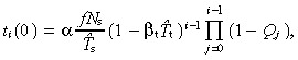(60)

where Q ₀ is defined to be 0. For convenience let us define the following equation

(61)

P ₀  = 1 because Q ₀  = 0 and P_g  = 0 because Q_g  = 1.

The density of all transit‐amplifying cells is given by equation 53, thus

(62)

With no apoptosis it is easily shown that this equation reduces to

(63)

The cell birth rate per unit area of skin surface is given by equation 55, and with suitable manipulation we get

(64)

If there is no apoptosis we get

(65)

The equations derived without variation in the number of transit generations can be derived from these more general equations by setting Q _i = 0 for i < g. This implies P _i = 1 for i < g.

Symmetric division For symmetric division the birth rate of i + 1 generation transit‐amplifying cells is twice that of asymmetric division (equation 59). Thus

t_{i +1} (0) = 2 t_i (0)(1 − β _t T̂ _t )(1 −  Q_i ). (66)

The solution of this is

(67)

Thus the density of all transit‐amplifying cells is

(68)

With no apoptosis it is easily shown that this equation reduces to

(69)

The cell birth rate per unit area of skin surface is given by equation 55

(70)

If there is no apoptosis we get

(71)

The equations for N _t and r for asymmetric and symmetric division, with and without apoptosis and with and without variation in number of transit generations are summarised in 2, 3, 4

Table 2.

Equations relating transit‐amplifying cell density and cell birth rate per unit area of skin surface to stem and transit‐amplifying cell kinetic parameters for asymmetric and symmetric division, with and without apoptosis and with and without variation in number of transit generations

Division	Lineage variation	Nt		r
		Without apoptosis	With apoptosis	Without apoptosis	With apoptosis
asym	no	(18)	(54)	(20)	(56)
	yes	(63)	(62)	(65)	(64)
sym	no	(26)	(57)	(28)	(58)
	yes	(69)	(68)	(71)	(70)

The equations for G _1‐8 are given in Table 3, and for α, T̂_s, T̂_t p _s(a), p_t(a) and P_i in Table 4. The number in parenthesis after each equation refers to the equation number in the text. These equations have been tested using numerical simulations with uniform and gamma distributions for the cell‐cycle times. The computer code, written in the C programming language, is available from the author.

Table 3.

Equations G_1‐8 used in Table 2 ; the equations for T̂_t and P_i are given in Table 4

Division	Lineage variation	Without apoptosis	With apoptosis
asym	no	G 1  =  g
	yes
sym	no	G 5  = 2 g  − 1
	yes

Table 4.

Equations for a, T̂_s, T̂_t, p_s(a), p_t(a) and P_i used in 2 , 3

(41)

(35)

(47)

(29)

(42)

(61)

The number in parenthesis after each equation refers to the equation number in the text.

CONSEQUENCES OF A HIERARCHICAL POPULATION STRUCTURE FOR EPIDERMIS

In this section we use the available experimental data on the epidermis to study the consequences of a hierarchical population structure. This is not easy for several reasons.

Firstly, until recently, there has been no marker that differentiates between stem and transit‐amplifying cells. Jones & Watt (1993) have shown that cells with high levels of surface β₁ integrins have properties characteristic of stem cells. These cells also rapidly adhere to type IV collagen, fibronectin and keratinocyte ECM. To use the mathematical models developed in this paper we must be able to differentiate between stem and transit‐amplifying cells.

Secondly, is a simple lack of data. We do not accurately know the density of stem or transit‐amplifying cells. There is no estimate for the proportion of cycling stem cells. We do not know the probability distributions of cell‐cycle times or variations in the number of transit generations. We do not know the rates of apoptosis. Moreover, different body sites have different parameter values.

Thirdly, some authors, as pointed out by Heenen & Galand (1997), treat the basal layer as the germinative compartment. While others think that suprabasal layers should be included. For example, Penneys et al. (1970) show that about 32% of mitoses can occur in suprabasal layers in normal human epidermis. The choice of which layers constitute the germinative compartment will affect the number of cells counted in an experiment, that is, N. This will affect, for example, estimates of cell birth rate (r) and growth fraction (GF).

Fourthly, the experimental data of hierarchical populations of cells has sometimes been interpreted using a homogeneous population model. At the least, this will make parameter estimates error prone. At worst, it will make estimates meaningless.

Finally, as pointed out by Dover & Wright (1991), there are numerous methodologies in the field, and it can be difficult to interpret measurements and assess their significance.

It is not the purpose of this paper to critically review the available experimental data: just to take the data at face value and say something about the consequences of a hierarchical population structure.

We first briefly review some of the experimental data. We then discuss the role of apoptosis, variation in the cell‐cycle times and variations in the number of transit generations. Finally, we discuss cell birth rate, growth fraction and their relationship.

A quick review of some data

The density of cells in the germinative compartment is estimated at N ∼ 44 000 cells mm⁻² (Weinstein et al. 1984). The fraction of stem cells in the germinative compartment (N _s/N) in normal human epidermis is estimated to be about 10% (Potten & Hendry 1973; Parkinson et al. 1984). This gives N _s ∼ 4400 cells mm⁻². The proportion of transit‐amplifying cells in humans is not known. In mice it is thought to be roughly 60% of the germinative compartment (Potten 1975).

There are estimated to be about 3‐5 transit generations in mice (Potten 1981; Jones & Watt 1993, , Jones et al. 1995). However, the probability distribution of transit generations is not known.

There are no conclusive, independent measurements of stem and transit‐amplifying cell parameters in humans. Measured cell‐cycle times vary between 30 and 300 h (Dover & Potten 1983). Stem cell‐cycle time in mice was estimated at 180 h and transit‐amplifying cell‐cycle time at 90 h (Potten & Bullock 1983).

There is currently no estimate for the fraction of cycling stem cells (f) in human or mouse.

The data of Loeffler et al. (1987) gave the best fit to an asymmetric division scheme in mice. Symmetric division, however, could not be conclusively ruled out. There is no data to suggest a division scheme in humans.

The growth fraction of human epidermis is thought to lie somewhere between 10 and 20% (Heenen et al. 1998) and that of mice around 60% (Iversen et al. 1968).

Weinstein et al. (1984 ) have estimated r to be about 1200 cells mm ⁻²  d ⁻¹ . However, this assumes that human epidermis has a growth fraction of 60% and a homogeneous population structure.

Apoptosis in normal and psoriatic epidermis

The apoptotic index is the number of apoptotic cells, divided by the total number of cells in the germinative compartment. It was measured in normal, stable psoriatic and regressing psoriatic epidermis (Laporte et al. 2000). The values found were 0.0012 ± 0.0002, 0.00035 ± 0.00004 and 0.0031 ± 0.0008, respectively. Because our models are only valid in equilibrium conditions, we will not use the data for regressing psoriatic epidermis.

The rate of apoptosis is given by the apoptotic index divided by the duration of apoptosis. To our knowledge, there has been no study on duration of apoptosis in keratinocytes. Therefore we use the value of 3 h given in Bursch et al. (1990). This gives rates of 4 × 10⁻⁴ h⁻¹ in normal skin and 1.2 × 10⁻⁴ h⁻¹ in psoriatic skin. We will assume, due to lack of evidence, that the rates of apoptosis in stem and transit‐amplifying cells are equal (that is, β_s = β_t = β).

In Fig. 4 we show how the rate of apoptosis affects the relative change in cell birth rate. In these graphs, we assume that the germinative compartment is in equilibrium and all other parameters are constant. This means that we do not suggest that cell birth rate will decline as apoptotic rate increases. The apoptotic rate may affect the other parameters that we do not account for in our models.

Figure 4.

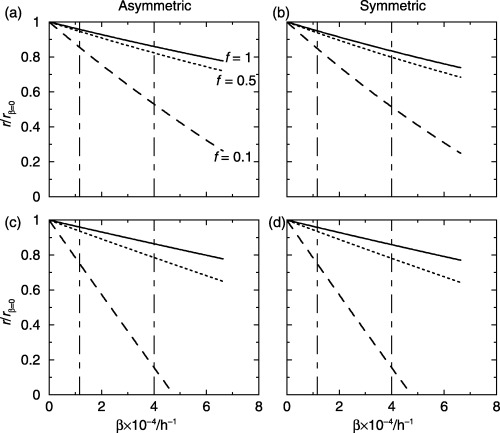
The effect of apoptosis on the cell birth rates per unit area of skin surface. The curves are the ratios of birth rate with apoptosis to birth rate without apoptosis. There is little difference between asymmetric and symmetric division, compare (a) with (b) and (c) with (d). (a,b) T̄ _s  = T̄ _t  = 100 h and (c,d) T̄ _s  = 200 h and T̄ _t  = 20 h, with β _s  = β _t  = β’ g  = 3, φ _s  = φ _t  = 0.1 and gamma distributed cell‐cycle times. The two vertical lines represent the apoptotic rates in normal (right) and psoriatic (left) skin.

In Fig. 4(a,b) the stem and transit‐amplifying cell‐cycle times have gamma distributions with T̄_s = T̄_t = and 100 h and φ_s = φ_t = 0.1. In Fig. 4(c and d), T̄_s = 200 h and T̄_t = and 20 h. Fig. 4(a and c) are for asymmetric division and Fig. 4(b and d) are for symmetric division.

There are several observations to note from Fig. 4. There is very little difference between symmetric and asymmetric division. The smaller the value of f the greater the relative change in cell birth rate for different apoptotic rates. The cell birth rate declines as the apoptotic rate increases. The change in cell birth rate from normal to psoriatic skin has the potential to be large, especially for low values of f. For example, a factor of six increase if f = 0.1 and T̄_s = 200 h and T̄_t = and 20 h.

Variation in cell‐cycle times

There is some evidence for large variations in the cell‐cycle times. For example, the coefficient of variation in human keratinocytes in vitro is 24% (Dover & Potten 1988), and in psoriasis 75% (Duffill et al. 1976). In many studies only point estimates are given for cell‐cycle times. Dover & Wright (1991) have rightly argued that it is essential to also give an interval estimate: a comparison of data from different studies is meaningless otherwise. Our models show that, if apoptosis is negligible, then we can use the average cell‐cycle times. However, if apoptosis is significant, using average values in incorrect. We must use the so‐called effective cell‐cycle times T̂_s and T̂_t.These parameters imply that the coefficients of variation of the cell‐cycle times also affect transit‐amplifying cell density and cell birth rate.

It is often assumed that the age structure of germinative cells is either rectangular or exponential. If there is variation in the cell‐cycle times then this assumption is wrong. Figure 2 shows an example of an age distribution for cells with a cell‐cycle time with a gamma distribution. Moreover, we must consider the age distributions of stem and transit‐amplifying cells separately. Combining all cells into a single age distribution does not allow us to predict anything from the mathematical models.

Variation in the number of transit generations

There is no evidence for or against variation in the number of transit generations. But if there is, what effect could it have on the parameters? To demonstrate the effect let us consider two simple examples with a maximum of three transit generations, without apoptosis and for asymmetric (Fig. 5a) and symmetric (Fig. 5b) division. For asymmetric division, r is given by equation 65. Writing r in terms of Q_i gives

Figure 5.

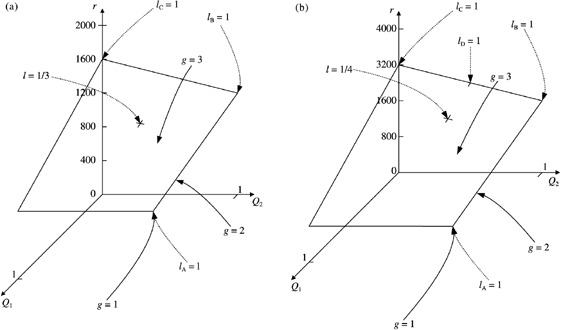
The effect of variation in the number of transit generations on cell birth rate per unit area of skin surface for a maximum of three generations, without apoptosis and with f  = 1, N _s  = 4000 cells mm ⁻² and T̄ = 100h for (a) asymmetric and (b) symmetric division. Birth rate is given by fN _s /T̄ _s  = (4 − 2 Q ₁  −  Q ₂  +  Q ₁ Q ₂ ) and fN _s /T̄ _s  = (8 − 6 Q ₁  − 4 Q ₂  + 4 Q ₁ Q ₂ )for asymmetric and symmetric division, respectively. When g  = 1 or g  = 2 the birth rate can also be read off from these graphs by setting Q ₁  =  Q ₂ = 1 or Q ₂  = 1, respectively. Also shown are points on the planes that correspond to specific values of the lineage frequencies from Fig. 4, i.e. l _A  = 1, l _B  = 1, l _C  = 1, l _D  = 1 and l _A  =  l _B  =  l _C  =  l  = 1/3 for asymmetric division and l _A  =  l _B  =  l _C  =  l _D  =  l  = 1/4 for symmetric division.

(72)

When g = 3, r can take any value on the plane defined by equation 72 and shown in Fig. 5a. When g = 2, Q ₂ = 1, that is, all second‐generation transit‐amplifying cells divide to give two post‐mitotic cells. Then r can take any value on the line fN _s/T̄_s(3 −Q ₁). When g = 1, Q ₁ = 1 and hence r = 2fN _s/T̄_s. If we had g = 4, then we would have to include a third parameter Q ₃. It is not possible to visualize this case because we would need a 4‐dimensional graph.

In Fig. 4 we show all the possible lineages for g = 3. We can map specific frequencies of these lineages onto the plane in Fig. 5a. When l _A = 1 (g = 1) then Q ₁ = Q ₂ = 1. When l _B = 1, Q ₁ = 0 and Q ₂ = 1. When l _C = 1, Q ₁ = Q ₂ = 0 and when l _A = l _B = l _C = l = 1/3, Q ₁ = 1/3 and Q ₂ = 1/2.

Similar results apply for symmetric division, except r is now given by equation 71. When written in terms of Q_i, this gives

(73)

When g = 3, r can take any value on the plane defined by equation 73 and shown in Fig. 5b. There is one extra lineage for symmetric division as shown in Fig. 4. When l _D = 1, Q ₁ = 0 and Q ₂ = 1/2. Also when l _A = l _B = l _C = l _D = l = 1/4, Q ₁ = 1/4 and Q ₂ = 1/2.

It is clear from Fig. 5 that variation in the number of transit generations can significantly affect cell birth rate.

Cell birth rate

If apoptosis is negligible and the epidermis in equilibrium, cell birth rate per unit area of skin surface (r) does not directly depend on the mean transit‐amplifying cell‐cycle time (T̄_t). This is because of two opposing effects. A change in T̄_t causes a proportional change in transit‐amplifying cell density N _t. But it causes an inversely proportional change in the rate transit‐amplifying cells divide.

However, we do not imply that mean transit‐amplifying cell‐cycle time has no effect on cell birth rate. It may have indirect effects on the other parameters – f, N _s, T̄_s and g. It is impossible to infer from our models how any two parameters co‐vary.

Reduced cell‐cycle times have often been put forward as a possible cause of hyperproliferation in psoriasis. The implication from this work is that reduced cell‐cycle times do not necessarily imply hyperproliferation. Evidence for no change in cell‐cycle times between normal and psoriatic skin has been provided by Van Ruissen et al. (1996). Another suggested cause for hyperproliferation in psoriasis is the large increase in the density of proliferative cells. However, the two may not be linked: an increase in transit‐amplifying cell‐cycle time increases transit‐amplifying cell density but not cell birth rate.

Growth fraction

Growth fraction is defined as the fraction of actively cycling cells in the germinative compartment

(74)

where N is the density of cells in the germinative compartment. Let us assume that apoptosis is negligible and there is no variation in transit generations. Substituting equation 18 into the above and solving for f, we get the following equation for asymmetric division

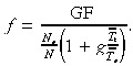(75)

Similarly for symmetric division we get

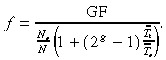(76)

The most recent data suggest that, in human forearm, the growth fraction lies somewhere between 10 and 20% (Heenen et al. 1998). As an example, let us assume that stem cells make up 10% of the germinative compartment (Potten & Hendry 1973; Parkinson et al. 1984) and that g = 3. In Fig. 6 we plot f against T̄_t/T̄_s for various growth fractions.

Figure 6.

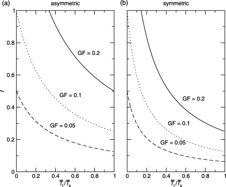
The fraction of cycling stem cells versus the ratio of the mean transit‐amplifying to the mean stem cell‐cycle times for different growth fractions for (a) asymmetric ( equation 75) and (b) symmetric ( equation 76) division. It is commonly thought that stem cells should have a longer cell‐cycle time than transit‐amplifying cells.

There are several observations to note from Fig. 6. Firstly, for these parameter values, if the growth fraction is 20%, there is a constraint on the cell‐cycle times due to f ≤ 1. For asymmetric division this constraint is T̄_s ≤ 1.7T̄_t, and for symmetric division it is T̄_s ≤ 4.4T̄_t. Secondly, if the growth fraction is less than 10%, f is always less than unity for all cell‐cycle time ratios and both division schemes. Conversely, if f = 1 the minimum growth fraction is 10%. Thirdly, if T̄_t ≤ T̄_s then there is a theoretical maximum growth fraction. For asymmetric division it is 40% and for symmetric division it is 80%.

In mice the growth fraction has been estimated to be about 60% (Iversen et al. 1968). With the same parameters as for human skin, this would imply that T̄_s ≤ 0.6T̄_t for asymmetric division and T̄_s ≤ 1.4T̄_t for symmetric division. It is generally considered that stem cells have a longer cell‐cycle time than transit‐amplifying cells in order to maintain genetic integrity. Thus, the model suggests that symmetric division is more likely in mouse epidermis. This contradicts the results of Loeffler et al. (1987). Their best fit to data suggested asymmetric division, although they could not rule out symmetric division.

Growth fraction, birth rate and cell‐cycle time

In a homogeneous population of cells, with no apoptosis, the cell birth rate is related to the growth fraction according to the following equation

(77)

where T _c is the mean cell‐cycle time.

This equation is widely used for hierarchical populations of cells even though it only holds for a homogeneous population. Is this correct? Consider the case when apoptosis is negligible. We have

(78)

and

(79)

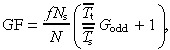
where G _odd is taken from Table 3. Combining these two equations we find that

(80)

This is obviously different from equation 77 due to differences in stem and transit‐amplifying cell‐cycle times.

When T̄_t = T̄_s then r′ = GF/T̄_s and we retrieve the equation for a homogeneous population. There is no reason, however, to assume that this is the case: it is thought that transit‐amplifying cells have a shorter cell‐cycle time than stem cells. When we include apoptosis, the equations become even more dissimilar. In conclusion, equation 77 should not be used to determine cell birth rate if the cell population has a hierarchical structure.

CONCLUSION

We have derived equations that relate various cell kinetic parameters of models of a hierarchical population of cells in equilibrium. The models include variation in cell‐cycle times, a stem cell G ₀ compartment, apoptosis and variation in the number of transit generations. The models are not mechanistic. Which means that we cannot say, for example, that decreasing apoptotic rate increases cell birth rate because the models do not tell us how decreasing the apoptotic rate affects the other parameters. What the models do, is predict how a set of parameters are related when the cell population is in equilibrium.

The models we have chosen to analyse have analytical solutions. The assumptions made for this to be so are debatable. Firstly, we assume that stem cells differentiate immediately after division. However, Dover & Watt (1987) have found that cells may differentiate other than during G ₁. Secondly, we assume that all proliferating stem cells are desynchronized in their cell‐cycle. However, neighbouring cells are likely to be related and hence closely synchronized. This assumption is weakened by considering a large number of stem cells. Thirdly, we do not consider circadian rhythms which have been shown to occur in mouse epidermis (Potten & Bullock 1983). Fourthly, we assume that the cell‐cycle times of daughter cells are not correlated, which has been shown to occur in cultured human keratinocytes (Dover & Potten 1988). Fifthly, we assume that there is no correlation between transit‐amplifying cell‐cycle times and the number of rounds of division. Whether this occurs or not is unknown. Sixthly, we assume that once a cell enters the cell‐cycle it always proceeds to division. This is not always the case with some cells arresting in the G ₂ phase (Ralfs et al. 1981). Finally, we have assumed that apoptosis occurs at the same rate throughout the cell‐cycle including G ₀. Evidence for or against this is lacking in keratinocytes.

Relaxing any of these assumptions will probably cause the models to be analytically intractable: leaving as our only recourse, numerical simulation and analysis. On a pessimistic note, it is doubtful that even the more complex equations derived in this paper are sufficient to model the kinetics of the germinative compartment due to the many simplifying assumptions made. Even if this is true, the process of deriving equations forces us to make explicit our assumptions, and in turn causes us to realize what we do not know.

The main conclusion of this work is that the simple equations derived for a homogeneous cell population should not be used for a hierarchical cell population. They can only be used when apoptosis is negligible and the mean stem and transit‐amplifying cell‐cycle times are equal. We cannot make these assumptions without further experimental work to test them. Another precautionary point; the distribution of cell‐cycle times of stem and transit‐amplifying cells must not be lumped together. To do so makes model testing impossible. Unfortunately there are no experimental techniques yet that can clearly distinguish between the two cell types.

The relative effect of apoptosis on cell birth rate depends on the values of the other cell kinetic parameters: especially the fraction of cycling stem cells. Moreover, if apoptosis is negligible then we need only consider average cell‐cycle times. If not, then we need more information about the distributions of cell‐cycle times – for example their coefficients of variation. Unfortunately, it is impossible to predict the importance of apoptosis from the available experimental data. Variation in the number of transit generations can also significantly affect cell birth rate. Finally, we have shown that cell birth rate does not directly depend on transit‐amplifying cell‐cycle times when the epidermis is in equilibrium.

APPENDIX A

Simplification of equation 7

Consider the integral

(A.1)

where

(A.2)

Substituting equation A.2 into equation A.1 we get

(A.3)

If f(x) is measurable then, by Tonelli's theorem, we can swap the order of the integrals (making sure that the limits are appropriately changed):

(A.4)

f ( x ) can be moved outside the inner integral:

(A.5)

Solving the inner integral gives

(A.6)

which equals x̄ the mean value of x.

APPENDIX B

Proof of equation 29

Say we did an experiment to count the number of stem cells that divided between ages a and a + δa. Firstly, let us assume that the stem cells do not undergo apoptosis. Let M(a)δa be the number of stem cells per unit area of skin surface that divided between ages a and a + δa. The total number of cell divisions per unit area of skin surface is . So the probability of a cell dividing between ages a and a + δa is

(B.1)

Now consider a similar population of stem cells that do undergo apoptosis. Let m(a)δa be the number of stem cells per unit area of skin surface that divided between ages a and a + δa. Therefore the probability of a cell dividing between ages a and a + δa is

(B.2)

What is the relationship between M(a)δa and m(a)δa? We assume that cells undergo apoptosis at a constant rate β_s throughout the cell cycle. This implies that the number of cells that divided
between ages a and a + δa has decayed by a factor compared with cells that do not undergo apoptosis, that is,

(B.3)

or

(B.4)

Substituting equation B.4 into equation B.1 we get

(B.5)

From equation B.2 we have

(B.6)

Substituting equation B.6 into equation B.5 we get

(B.7)

Multiplying both sides of equation B.2 by gives

(B.8)

and integrating gives

(B.9)

Substituting the right hand side of equation B.9 into equation B.7 gives

(B.10)

APPENDIX C

Simplification of equation 34

Consider the integral

(C.1)

where

(C.2)

Substituting equation C.2 into equation C.1 we get

(C.3)

Moving e ^−βy inside the inner integral:

(C.4)

If f(x) is measurable then, by Tonelli's theorem, we can swap the order of the integrals (making sure that the limits are appropriately changed):

(C.5)

f ( x ) can be moved outside the inner integral, which can now be solved:

(C.6)

and simplified:

(C.7)

REFERENCES

- Albers KM, Setzer RW, Taichman LB (1986) Heterogeneity in the replicating population of cultured human epidermal keratinocytes. Differentiation 31, 134. [DOI] [PubMed] [Google Scholar]
- Appleton DR, Wright NA, Dyson P (1977) The age distribution of cells in stratified squamous epithelium. J. Theor. Biol. 65, 769. [DOI] [PubMed] [Google Scholar]
- Barrandon Y, Green H (1985) Cell size as a determinant of the clone forming ability of human keratinocytes. PNAS 82, 5390. [DOI] [PMC free article] [PubMed] [Google Scholar]
- Barrandon Y, Green H (1987) Three clonal types of keratinocytes with different capacities for multiplication. PNAS 84, 2302. [DOI] [PMC free article] [PubMed] [Google Scholar]
- Bursch W, Kleine K, Tenniswood M (1990) The biochemistry of cell death by apoptosis. Biochem. Cell Biol. 68, 1071. [DOI] [PubMed] [Google Scholar]
- Clausen OPF, Kirkhus B, Thorud E, Schjolberg A, Moen E, Cromarty A (1986) Evidence of mouse epidermal subpopulations with different cell cycle times. J. Invest. Dermatol. 86, 266. [DOI] [PubMed] [Google Scholar]
- Dover R, Potten CS (1983) Cell cycle kinetics of cultured human epidermal keratinocytes. J. Invest. Dermatol. 80, 423. [DOI] [PubMed] [Google Scholar]
- Dover R., Potten CS (1988) Heterogeneity and cell cycle analyses from time‐lapse studies of human keratinocytes in vitro . J. Cell. Sci. 89, 359. [DOI] [PubMed] [Google Scholar]
- Dover R, Watt FM (1987) Measurement of the rate of epidermal terminal differentiation: expression of involucrin by S‐phase keratinocytes in culture and in psoriatic plaques. J. Invest. Dermatol. 89, 349. [DOI] [PubMed] [Google Scholar]
- Dover R, Wright NA (1991) The cell proliferation kinetics of the epidermis In: Goldsmith LA, ed. Physiology, Biochemistry and Molecular Biology of the Skin, p. 239 Oxford: Oxford University Press. [Google Scholar]
- Duffill M, Wright NA, Shuster S (1976) The cell proliferation kinetics of psoriasis examined by three in vivo techniques. Br. J. Dermatol. 94, 355. [DOI] [PubMed] [Google Scholar]
- Heenen M, Galand P (1997) The growth fraction of normal human epidermis. Dermatology 194, 313. [DOI] [PubMed] [Google Scholar]
- Heenen M, Thiriar S, Noël JC, Galand P (1998) Ki‐67 immunostaining of normal human epidermis: comparison with 3H‐thymidine labelling and PCNA immunostaining. Dermatology 197, 123. [DOI] [PubMed] [Google Scholar]
- Holbrook KA (1994) Ultrastructure of the epidermis In: Leigh IM, Lane B, Watt FM, eds. The Keratinocyte Handbook, p. 3 London: Cambridge University Press. [Google Scholar]
- Iversen O, Bjerknes R, Devik R (1968) Kinetics of cell renewal, cell migration and cell loss in the hairless mouse dorsal epidermis. Cell Tissue Kinet. 1, 365. [Google Scholar]
- Jensen PKA, Pedersen S, Bolund L (1985) Basal cell subpopulations and cell cycle kinetics in human epidermal explant cultures. Cell Tissue Kinet. 18, 207. [DOI] [PubMed] [Google Scholar]
- Jensen UB, Lowell S, Watt FM (1999) The spatial relationship between stem cells and their progeny in the basal layer of human epidermis: a new view based on whole‐mount labelling and lineage analysis. Development 126, 2409. [DOI] [PubMed] [Google Scholar]
- Jones PH, Harper S, Watt FM (1995) Stem cell patterning and fate in human epidermis. Cell 80, 83. [DOI] [PubMed] [Google Scholar]
- Jones PH, Watt FM (1993) Separation of human epidermal stem cells from transit amplifying cells on the basis of differences in integrin function and expression. Cell 73, 713. [DOI] [PubMed] [Google Scholar]
- Laporte M, Heenen M (1994) The heterogeneity of the germinative compartment in human epidermis and its implications in pathogenesis. Dermatology 189, 340. [DOI] [PubMed] [Google Scholar]
- Laporte M, Galand P, Fokan D, De G raef C, Heenen M (2000) Apoptosis in established and healing psoriasis. Dermatology 200, 314. [DOI] [PubMed] [Google Scholar]
- Leigh RM, Pulford KA, Ramaekers FCS, Lane EB (1985) Psoriasis: maintenance of an intact monolayer basal cell differentiation compartment in spite of hyperproliferation. Br. J. Dermatol. 113, 53. [DOI] [PubMed] [Google Scholar]
- Loeffler M, Potten CS, Wichmann HE (1987) Epidermal cell proliferation. II. A comprehensive mathematical model of cell proliferation and migration in the basal layer predicts some unusual properties of epidermal stem cells. Virchows Arch. B 53, 286. [PubMed] [Google Scholar]
- Parkinson EK, Pera MF, Emmerson A, Gorman PA (1984) Differential effects of complete and second‐stage tumour promoters in normal but not transformed human and mouse keratinocytes. Carcinogenesis 5, 1071. [DOI] [PubMed] [Google Scholar]
- Penneys NS, Fulton JE, Weistein GD, Frost P (1970) Location of proliferating cells in human epidermis. Arch. Dermatol. 101, 323. [PubMed] [Google Scholar]
- Potten CS (1974) The epidermal proliferative unit: the possible role of the central basal cell. Cell Tissue Kinet. 7, 77. [DOI] [PubMed] [Google Scholar]
- Potten CS (1975) Epidermal cell production rates. J. Invest. Dermatol. 65, 488. [DOI] [PubMed] [Google Scholar]
- Potten CS (1976) Location of clonogenic cells in the epidermis and the structural arrangements of the epidermal proliferative unit In: Cairnie AB, Lala PK, Osmond S, eds. Stem Cells of Renewing Cell Populations, p. 91 New York: Academic Press. [Google Scholar]
- Potten CS (1981) Cell replacement in epidermis (keratopoiesis) via discrete units of proliferation. Int. Rev. Cytol. 69, 271. [DOI] [PubMed] [Google Scholar]
- Potten CS, Bullock JC (1983) Cell kinetic studies in the epidermis of the mouse. I. Changes in labeling index with time after tritiated thymidine administration. Experientia 39, 1125. [DOI] [PubMed] [Google Scholar]
- Potten CS, Hendry JH (1973) Clonogenic cells and stem cells in epidermis. Int. J. Radiat. Biol. 24, 537. [DOI] [PubMed] [Google Scholar]
- Potten CS, Loeffler M (1987) A comprehensive model of the crypts of the small intestine of the mouse provides insight into the mechanisms of cell migration and the proliferation hierarchy. J. Theor. Biol. 127, 381. [DOI] [PubMed] [Google Scholar]
- Potten CS, Loeffler M (1990) Stem cells: attributes, cycles, spirals, pitfalls and uncertainties. Lessons for and from the crypt. Development 110, 1001. [DOI] [PubMed] [Google Scholar]
- Potten CS, Wichmann HE, Loeffler M, Dobek K, Major D (1982) Evidence for discrete cell kinetic populations in mouse epidermis based on mathematical analysis. Cell Tissue Kinet. 15, 305. [DOI] [PubMed] [Google Scholar]
- Ralfs I, Dawber R, Ryan T, Duffill M, Wright NA (1981) The kinetics of metaphase arrest in human psoriatic epidermis: an examination of optimal experimental conditions for determining the birth rate. Br. J. Dermatol. 104, 231. [DOI] [PubMed] [Google Scholar]
- Van Ruissen F, De Jongh GJ, Van Erp PEJ, Boezeman JBM, Schalkwijk J (1996) Cell kinetic characterization of cultured human keratinocytes from normal and psoriatic individuals. J. Cell Physiol. 168, 684. [DOI] [PubMed] [Google Scholar]
- Watt FM (1988) Epidermal stem cells: markers, patterning and the control of stem cell fate. Phil. Trans. R. Soc. Lond. B 353, 831. [DOI] [PMC free article] [PubMed] [Google Scholar]
- Weinstein GD, McCullough JL, Ross P (1984) Cell proliferation in normal epidermis. J. Inves. Dermatol. 82, 623. [DOI] [PubMed] [Google Scholar]