DIABLO: an integrative approach for identifying key molecular drivers from multi-omics assays

Abstract

Motivation

In the continuously expanding omics era, novel computational and statistical strategies are needed for data integration and identification of biomarkers and molecular signatures. We present Data Integration Analysis for Biomarker discovery using Latent cOmponents (DIABLO), a multi-omics integrative method that seeks for common information across different data types through the selection of a subset of molecular features, while discriminating between multiple phenotypic groups.

Results

Using simulations and benchmark multi-omics studies, we show that DIABLO identifies features with superior biological relevance compared with existing unsupervised integrative methods, while achieving predictive performance comparable to state-of-the-art supervised approaches. DIABLO is versatile, allowing for modular-based analyses and cross-over study designs. In two case studies, DIABLO identified both known and novel multi-omics biomarkers consisting of mRNAs, miRNAs, CpGs, proteins and metabolites.

Availability and implementation

DIABLO is implemented in the mixOmics R Bioconductor package with functions for parameters’ choice and visualization to assist in the interpretation of the integrative analyses, along with tutorials on http://mixomics.org and in our Bioconductor vignette.

Supplementary information

Supplementary data are available at Bioinformatics online.

1 Introduction

Technological improvements have allowed for the collection of data from different molecular compartments (e.g. gene expression, DNA methylation status, protein abundance) resulting in multiple omics (multi-omics) data from the same set of biospecimens or individuals (e.g. transcriptomics, proteomics, metabolomics). Systems biology approaches, by incorporating data from multiple biological compartments, provide improved biological insights compared with traditional single omics analyses (Kim et al., 2013; Wang et al., 2014; Zhu et al., 2012). One reason might be that interactions between omics layers is not taken into account in single omics analysis and prevents the reconstruction of accurate molecular networks. These molecular networks are dynamic, changing under perturbed conditions such as disease, response to therapy and environmental exposures. Therefore, adopting a holistic approach by integrating multi-omics data may bridge this information gap, and uncover networks that are representative of the underlying molecular mechanisms (Ritchie et al., 2015; Yugi et al., 2016).

Many strategies (component-based, message-passing, Bayesian methods, network analysis, classification schemes) have been proposed for multi-omics data integration to answer various questions, incorporating experimental data as well as curated data from biological databases (see Supplementary Fig. S1; Bersanelli et al., 2016; Huang et al., 2017; Meng et al., 2016; Ritchie et al., 2015; Rohart et al., 2017; Zeng and Lumley, 2018). These include data-driven methods for identifying novel phenotypic clusters such as Similarity Network Fusion (Wang et al., 2014), Bayesian Consensus Clustering (Kirk et al., 2012), and methods for extracting common sources of variation: joint Non-negative Matrix Factorization (Zhang et al., 2012), Joint and Individual Variation Explained (JIVE) (Lock et al., 2013), sparse MultiBlock Partial Least Squares (Li et al., 2012), regularized and sparse generalized canonical correlation analysis (sGCCA) (Tenenhaus and Tenenhaus, 2011; Tenenhaus et al., 2014) and Multi-Omics Factor Analysis (MOFA) (Argelaguet et al., 2018). Other methods such as Passing Attributes between Networks for Data Assimilation (Glass et al., 2013), Sparse Network regularized Multiple Non-negative Matrix Factorization (Zhang et al., 2011) and Reconstructing Integrative Molecular Bayesian NETworks (Zhu et al., 2012) can be used to incorporate curated data with experimental data in order to reconstruct biological networks. All of these methods are examples of unsupervised multi-omics data integration, that is, without the need of sample labels that categorize samples based on a certain phenotype or trait. However, researchers are also interested in multi-omics biomarkers that are predictive of disease, i.e. supervised methods in which molecular patterns that span across biological domains explain or characterize a known phenotype.

Supervised data integration approaches for the classification of multiple phenotypes (e.g. PAM50 breast cancer phenotypes) include multi-step approaches that concatenate all data prior to applying a classification model, or ensemble-based in which a classification model is applied separately to each omics data and the resulting predictions are combined based on average or majority vote (Günther et al., 2012). These approaches can be biased toward certain omics data types and do not account for interactions between omics layers (Aben et al., 2016; Ma et al., 2016). Recently, classification approaches such as Network smoothed t-statistics Support Vector Machines (Cun and Fröhlich, 2013), Generalized Elastic Net (Sokolov et al., 2016) and adaptive Group-Regularized ridge regression (van de Wiel et al., 2016) have incorporated curated biological data such as protein protein interactions (PPI) data, genetic pathway data and type of methylation probes. These methods are still limited to single omics data such that, either the concatenation or ensemble-based schemes must be applied to incorporate additional data types. Other approaches include The Analysis Tool for Heritable and Environmental Network Associations based on a Grammatical Evolution Neural Network that integrates multi-omics data for the prediction of clinical outcomes (Kim et al., 2013). However, the approach requires initial filtering, feature selection and modeling independently on each omics dataset prior to integration.

We introduce Data Integration Analysis for Biomarker discovery using Latent cOmponents (DIABLO), a multi-omics method that simultaneously identifies key omics variables (mRNA, miRNA, CpGs, proteins, metabolites etc.) during the integration process and discriminates phenotypic groups. DIABLO maximizes the common or correlated information between multiple omics datasets. It is the first multivariate integrative classification method of its kind that builds a predictive model for prediction on new samples. The method is based on Projection to Latent Structures (PLS), allowing for powerful visualizations. DIABLO is highly flexible in the type of experimental design it can handle, ranging from classical single time point to cross-over and repeated measures studies. Modular-based analysis can also be incorporated using pathway-based module matrices (Langfelder and Horvath, 2008) instead of the original omics matrices. We demonstrate the capabilities and versatility of DIABLO below, both in simulated and real multi-omics studies to identify relevant biomarkers of various diseases.

2 Materials and methods

2.1 General multivariate integrative framework

DIABLO extends sGCCA (Tenenhaus et al., 2014) to a classification or supervised framework. sGCCA is a multivariate dimension reduction technique that uses singular value decomposition and selects co-expressed (correlated) variables from several omics datasets. sGCCA maximizes the covariance between linear combinations of variables (latent component scores) and projects the data into the smaller dimensional subspace spanned by the components. The selection of the correlated molecules across omics levels is performed internally with ${\ell }_1$ penalization on the variable coefficient vector defining the linear combinations. Since all latent components are scaled in the algorithm, sGCCA maximizes the correlation between components. However, we will retain the term ‘covariance’ instead of ‘correlation’ throughout this section to present the general sGCCA framework.

Denote Q normalized, centered and scaled datasets $X^{(1)}(N\times P_1),X^{(2)}(N\times P_2)$,…, $X^{(Q)}(N\times P_Q)$ measuring the expression levels of $P_1,\dots ,P_Q$ ‘omics variables on the same N samples’. sGCCA solves the optimization function for each dimension $h=1,\dots ,H$:

$$\begin{array}{c}\underset{a_h^{(1)},\dots ,a_h^{(Q)}}{\max }{\displaystyle \sum _{i,\hspace{0.17em}j=1,\hspace{0.17em}i\ne j}^Q{c}_{i,j}}\text{ cov}(X_h^{(i)}{a}_h^{(i)},X_h^{(j)}{a}_h^{(j)}),\\ \text{s}.\text{t}.\left|\right|a_h^{(q)}|{|}_2=1\mathrm{a}\mathrm{n}\mathrm{d}|\left|a_h^{(q)}\right|{|}_1\le {\lambda }^{(q)}forall1\le q\le Q\end{array}$$ (1)

where $a_h^{(q)}$ is the variable coefficient or loading vector on dimension h associated to the residual matrix $X_h^{(q)}$ of the dataset $X^{(q)}$. $C={\left\{c_{i,j}\right\}}_{i,j}$ is a (Q × Q) design matrix that specifies whether datasets should be connected. Elements in C can be set to zeros when datasets are not connected and ones where datasets are fully connected, as we further describe in Section 2.2. In addition in (1), ${\lambda }^{(q)}$ is a non-negative parameter that controls the amount of shrinkage and thus the number of non-zero coefficients in $a_h^{(q)}$. Similar to the LASSO (Tibshirani, 1996) and other ${\ell }_1$ penalized multivariate models developed for single omics analysis (Lê Cao et al., 2011), the penalization enables the selection of a subset of variables with non-zero coefficients that define each component score $t_h^{(q)}=X_h^{(q)}{a}_h^{(q)}$. The result is the identification of variables that are highly correlated between and within omics datasets.

The sGCCA model (1) is iterative; a first set of coefficient vectors $(a_1^{(1)},\dots a_1^{(Q)})$ is obtained by maximizing (1) for h = 1 with $X_1^{(q)}=X^{(q)}$, before maximizing (1) for h = 2 using residual matrices $X_2^{(q)}=X_1^{(q)}-t_1^{(q)}{a}_1^{(q)},1\hspace{0.17em}\le \hspace{0.17em}q\hspace{0.17em}\le \hspace{0.17em}Q$. This process is repeated until a sufficient number of dimensions (or set of components) is obtained. The underlying assumption of sGCCA is that the major source of common biological variation can be extracted via the first set of component scores $t_1^{(q)},\dots ,t_h^{(Q)}$, while any unwanted variation due to heterogeneity across the datasets $X^{(q)}$ does not impact the statistical model. The optimization problem (1) is solved using a monotonically convergent algorithm (Tenenhaus et al., 2014).

2.2 DIABLO: supervised analysis and prediction

To extend sGCCA for a classification framework, we substitute one omics dataset $X^{(q)}$ in (1) with a dummy indicator matrix Y (N × G) to indicate the class membership of each sample, where G is the number of phenotype groups. For easier use of DIABLO, we replaced the ${\ell }_1$ penalty parameter ${\lambda }^{(q)}$ by the number of variables to select in each dataset and each component, as there is a direct correspondence between both parameters.

2.2.1 Input data

While DIABLO does not assume particular data distributions, all datasets should be normalized appropriately according to each omics platform and pre-processed if necessary (see the normalization steps described in Supplementary Section S2 for each case study). Samples should be represented in rows in the data matrices and match the same samples across omics datasets. The phenotype outcome y is a factor indicating the class membership of each sample and is internally transformed into a dummy matrix Y in mixOmics. In addition, each variable is centered and scaled internally, as is conventionally performed in PLS-based models. A multilevel variance decomposition option is available for repeated measures and cross-over study designs, as illustrated in the asthma study (Section 3.4).

2.2.2 Design matrix

The design matrix C is a (Q × Q) matrix with values ranging from 0 to 1, which specifies whether datasets should be connected, see (1). In our simulation study, we evaluated two scenarios: a null design (DIABLO_null) when no omics datasets are connected, and a full design when all datasets are connected (DIABLO_full):

$$C_{\text{null}}=\left[\begin{array}{lll}0\hfill & 0\hfill & 0\hfill \\ 0\hfill & 0\hfill & 0\hfill \\ 0\hfill & 0\hfill & 0\hfill \end{array}\right]C_{\text{full}}=\left[\begin{array}{lll}0\hfill & 1\hfill & 1\hfill \\ 1\hfill & 0\hfill & 1\hfill \\ 1\hfill & 1\hfill & 0\hfill \end{array}\right]$$

Every dataset is then connected to the outcome Y internally. For the two case studies Breast cancer and Asthma the design matrix was chosen based on our proposed method (see parameters tuning in Section 2.3). Note that the design matrix is not restricted to 0 and 1 values only and a compromise between correlation and discrimination can also be modeled as described in Rohart et al. (2017).

2.2.3 Consensus class prediction for each new sample

For a new sample, a set of H predicted component scores ($t_{1,\text{new}}^{(q)},\dots ,t_{H,\text{new}}^{(q)}$) can be calculated for each type of omics q by using the estimated loadings vectors $a^{(q)}$ from DIABLO. The predicted class of a new sample for each dataset is obtained from the predicted score using one of the distances Maximum, Centroids or Mahalanobis as detailed in Rohart et al. (2017), which results in Q class memberships for a new sample.

Since the different omics datasets may not all agree on a predicted class, a consensus class membership is determined using either a majority vote, a weighted majority vote or by averaging all $t_{h,\text{new}}^{(q)}$ for each component h across all Q datasets then applying a prediction distance scheme. In case of ties in the majority vote scheme, ‘NA’ is allocated as a prediction but is counted as a misclassification error during the performance evaluation. For the weighted majority vote, each omics dataset is weighted by the correlation between its latent components and the outcome, that is, stronger predictive datasets are up-weighted as compared with weaker omics datasets. As the class prediction relies on individual vote from each omics set, DIABLO allows for some missing datasets X_k during the prediction step, as illustrated in the Breast Cancer case study. We used the Centroid distance for the weighted majority vote scheme (Breast Cancer study) and the Maximum distance for the average vote scheme (asthma study) as those led to best performance (see Rohart et al., 2017 for details about distance measures and proposed voting schemes).

2.3 Parameters tuning

There are three types of parameters to tune in DIABLO.

• The design matrix C can be determined using either prior biological knowledge, or a data-driven approach. The latter approach can use PLS that models pair-wise associations between omics datasets (Lê Cao et al., 2008). If the correlation between the first component of each omics dataset is above a given threshold (e.g. 0.8) then a connection between those datasets is included in C as a 1 value.

• The number of components: in several analyses we found that $G-1$ components could extract sufficient information to discriminate all phenotype groups (Lê Cao et al., 2011), but this can be assessed by evaluating the model performance across all specified components, as described below, and can be aided with graphical outputs such as sample plots to visualize the discriminatory ability of each component.

• The number of variables to select per dataset and per component. A grid composed of a small number of variables (<50 with steps of 5 or 10) may suffice as we did not observe substantial changes in the classification performance during our case study analyses. The variable selection size can also be guided according to the downstream biological interpretation. For example, a gene set enrichment analysis may require a larger set of features than a literature-search interpretation.

2.4 DIABLO visualization outputs

To facilitate the interpretation of the integrative analysis, several types of graphical outputs were proposed and implemented in mixOmics.

Sample plots include a consensus plot that depicts the samples by calculating the average of the components from each dataset (Fig. 3A). Omics-specific sample plots can also be obtained by plotting components associated to each dataset (Supplementary Fig. S14).

Fig. 3.

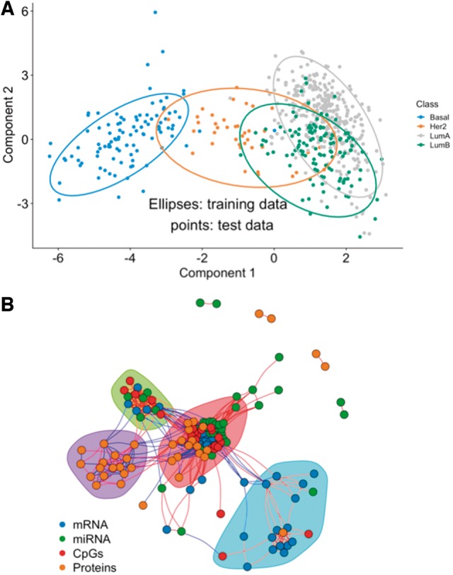
A multi-omics biomarker panel predictive of breast cancer subtypes. (A) DIABLO consensus component plot based on the identified multi-omics biomarker panel: test samples are overlaid with 95% confidence ellipses calculated from the training data. (B) Network visualization of the biomarker panel highlighting correlated variables (absolute Pearson’s correlation >0.4) and four communities based on the edge betweenness index

Variable plots give more insights into the variables that were selected by DIABLO. Our new circos plot represents correlations between and within selected variables from each dataset. The association between variables is computed using a similarity score that is analogous to a Pearson correlation coefficient (see González et al., 2012); this association is displayed as a color-coded link inside the plot to represent a positive or negative correlation above a user-specified threshold. The selected variables are represented on the side of the plot, with side colors indicating each omics type, optional line plots represent the expression levels in each phenotypic group (Supplementary Fig. S20).

Clustered image maps based on the Euclidean distance and the complete linkage display an unsupervised clustering between the selected variables (centered and scaled) and the samples (Supplementary Fig. S15). Color bars represent the sample phenotypic groups (columns) and the type of omics (rows) variables (see González et al., 2012).

3 Results

3.1 Correlation and discrimination tradeoff

Three omics datasets consisting of 200 samples (100 in each of the 2 phenotypic groups) and 260 variables were simulated (details in Supplementary Section S1). Each dataset included four types of variables: 30 correlated-discriminatory (corDis), 30 uncorrelated-discriminatory (unCorDis), 100 correlated-nondiscriminatory (corNonDis) and 100 uncorrelated-nondiscriminatory (unCorNonDis) variables. DIABLO models with either a null or full design (DIABLO_null, DIABLO_full), each with one component set and selecting 60 variables per dataset (180 in total), were compared with existing integrative classification schemes based on classification performance (10-fold cross-validation (CV), averaged over 20 simulations) and variable selection (Fig. 1). The covariance between datasets was held constant, with fold-change (FC) varying from 0 to 2, and noise (SD) between 0.2 and 1. When FC = 0, the error rate was ∼50% for all methods regardless of noise level (Supplementary Fig. S2). When FC = 1, DIABLO_full yielded a higher error rate than all other methods, for noise <1. However, when noise = 1 and FC = 1, all methods performed similarly. Finally, when FC = 2 (higher than both the covariance and noise levels) the error rate of the DIABLO_full model decreased further. We hypothesized that the increased error rate between the DIABLO models was due to the covariance constraint used to extract a common source of variation across datasets instead of independent sources of variation from each dataset. Therefore, we varied the covariance value between datasets and performed similar comparisons as described in Supplementary Figure S3. We found that increasing the covariance between datasets significantly increased the error rate for DIABLO_full, but not for DIABLO_null. When we added a second component set in DIABLO, allowing for additional independent information to be included, the classification performance improved and yielded similar results in both DIABLO designs. We hence concluded from this simulation study that the design in DIABLO achieves a tradeoff between correlation and discrimination. DIABLO_null focuses on selecting discriminatory variables and disregards most of the correlation between datasets, whereas DIABLO_full selects highly correlated and discriminatory variables across all datasets. Variables selected by DIABLO_full reflect the correlation structure between biological datasets, and may provide a balance between prediction accuracy and biological insight, as described in the next sections.

Fig. 1.

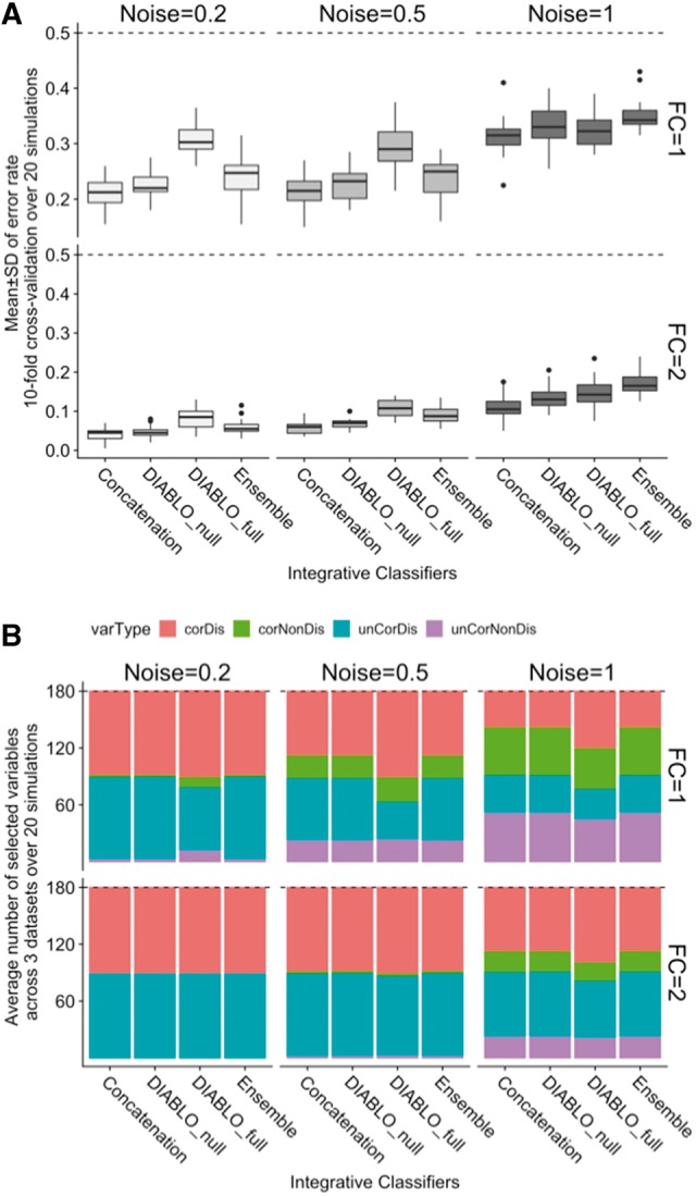
Simulation study. (A) Classification error rates (10-fold CV averaged over 20 simulations) for different FCs between groups and varying level of noise (SD). Dashed line indicates a random performance (error rate = 50%). (B) Types of variables selected by the different classification methods amongst the 180 variables selected for each classification method

3.2 Benchmark: DIABLO identifies highly interconnected networks with superior biological enrichment

We applied various integrative approaches to cancer multi-omics datasets (mRNA, miRNA, and CpG): colon, kidney, glioblastoma (gbm) and lung, to identify multi-omics biomarker panels predictive of high and low survival times (Table 1 ; Supplementary Section S2) and studied the network properties and biological enrichment of the selected features. Component-based integrative approaches were compared: supervised methods included concatenation and ensemble-based schemes using sparse partial least squares discriminant analysis (sPLSDA; Lê Cao et al., 2011), DIABLO_null and DIABLO_full, and unsupervised approaches included sGCCA, MOFA (Argelaguet et al., 2018), and JIVE (Lock et al., 2013), see Supplementary Section S3 for parameter settings. Each biomarker panel consisted of 180 features across two components (based on 90 variables with the largest weights on each of the 2 components). Across all cancer datasets, the largest overlap between biomarker panels was observed between all supervised methods with the exception of DIABLO_full whose selection was more similar to those identified with unsupervised methods (Fig. 2A; Supplementary Fig. S5 for the other studies). Interestingly, we observed similarities between the features identified by DIABLO_full and the unsupervised integrative approaches based on the following characteristics: (i) correlation between features—a large number of connections or edges regardless of the correlation cutoff was observed (Fig. 2B; Supplementary Fig. S6); (ii) network attributes such as high graph density, low number of communities and large number of triads (Supplementary Fig. S7) and (iii) small number of densely connected modules (Fig. 2C; Supplementary Fig. S8). The tradeoff in selecting correlated features by DIABLO_full was at a slight expense of discrimination, as can be observed in the component plots that depict the separation of the high and low survival groups (Fig. 2C; Supplementary Fig. S9). DIABLO_null also achieved a good separation of the survival groups, but with biomarker panel characteristics similar to those of other supervised methods. Internal validation on the benchmark datasets showed that DIABLO_null led to better cluster consistency according to phenotypic groups compared with all other methods (Supplementary Fig. S10).

Table 1.

Overview of multi-omics datasets analyzed for method benchmarking and in two case studies

Dataset	n	Omics	p
Colon	92	mRNA	17 814
Wang et al. (2014)	High: 33	miRNA	312
	Low: 59	CpGs	23 088
Kidney	122	mRNA	17 665
Wang et al. (2014)	High: 61	miRNA	329
	Low: 61	CpGs	24 960
Glioblastoma	213	mRNA	12 042
Wang et al. (2014)	High: 105	miRNA	534
	Low: 108	CpGs	1305
Lung	106	mRNA	12 042
Wang et al. (2014)	High: 53	miRNA	353
	Low: 53	CpGs	23 074
Breast Cancer	989	mRNA	16 851
TCGA Research Network (2012)	Basal: 76 (102)	miRNA	349
	Her2: 38 (40)	CpGs	9482
	LumA: 188 (346)	Proteins	115 (0)
	LumB: 77 (122)
Asthma	28	Cell types	9
Singh et al. (2013, 2014)	Pre: 14	mRNA modules	229
	Post: 14	Metabolite modules	60

Note: The breast cancer case study includes training (test) datasets for all omics types except proteins.

Fig. 2.

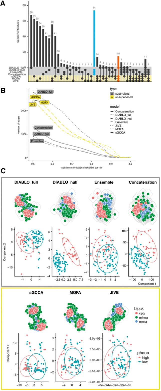
Benchmark for colon cancer. (A) Number of selected features overlapping between supervised and unsupervised methods. (B) Number of correlated variables in the biomarker panels for various Pearson correlation cutoffs. (C) Top: network modularity of each multi-omics biomarker panel. Gray circles depict modules based on the edge betweenness index from the igraph R-library. Bottom: consensus component plots depicting the separation of subjects in the high and low survival groups. Similar patterns were observed for kidney, gbm and lung cancer datasets, see Supplementary Figures S5–S10

Gene set enrichment analysis based on hypergeometric tests were conducted on each biomarker panel. Briefly, we used gene symbols of mRNAs and CpGs of each biomarker panel and gene sets from 10 collections such a positional, curated, motif, computational, Gene Ontology, ontologic, immunologic, and hallmark gene sets as well as blood transcriptional modules and cell-specific gene sets (Supplementary Section S4). DIABLO_full identified the greatest number of significant gene sets (False Discovery Rate (FDR) = 5%) across the gene set collections and generally ranked higher than the other methods in colon (7 collections), gbm (5) and lung (5) cancer datasets (Supplementary Table S1). JIVE outperformed all methods in the kidney cancer datasets (six collections). In conclusion for this benchmark study, DIABLO_full aims at explaining the correlation structure between multiple omics layers and the phenotype of interest, leading to the greatest number of known biological gene sets such as pathway, functions and processes.

3.3 Competitive performance and identification of known and novel multi-omics biomarkers of breast cancer subtypes

On the TCGA breast cancer study we focused our analyses on characterizing and predicting PAM50 breast cancer subtypes. Processing and normalization is described in Supplementary Section S2 and Fig. S11.

3.3.1 Classification performance benchmark

First, we compared the classification error rates of DIABLO models (DIABLO_null and DIABLO_full) with existing classification schemes (Concatenation and Ensemble) using sPLSDA and Elastic Net (enet) classifiers. For the purposes of this comparative performance analysis, the proteomics dataset that was only available for the training set was excluded to address the limitation of the Concatenation-based scheme. Hyperparameters for all six classifiers were tuned on the training set (mRNA, miRNA, CpGs) using 5-fold CV repeated five times and a variable selection size grid approach on three components (Concatenation, Ensemble) or three component sets (DIABLO). The performance of the methods was assessed on the independent test set (see Supplementary Section S5 for details). DIABLO_null and DIABLO_full led to a classification error rate of 19 and 21%, respectively, while Concatenation and Ensemble-based methods error rate ranged from 11 to 28% (Supplementary Table S2, all methods included three component sets). We noted that Concatenation-based classifiers tended to be biased towards the more predictive variables (mRNA or CpGs), whereas DIABLO selected variables evenly across datasets and had similar error rates between training and test datasets.

3.3.2 Identification of multi-omics biomarkers

We then applied DIABLO_full for variable selection and evaluated its prediction performance on all omics available (mRNA, miRNA, CpGs and proteins). The optimal multi-omics biomarker panel size was identified as described above and detailed in Supplementary Figure S12. Our panel consisted of 45 mRNA, 45 miRNAs, 25 CpGs and 55 proteins selected across three component sets with a balanced error rate (BER; see Rohart et al., 2017) of 17.9 ± 1.9%. This panel identified many variables with previously known associations with breast cancer, according to MolSigDB (Liberzon et al., 2015), miRCancer (Xie et al., 2013), Online Mendelian Inheritance in Man (Hamosh et al., 2005) and DriverDBv2 (Chung et al., 2016). In addition, we identified several variables that were not found in any database and that may represent novel biomarkers of breast cancer (Supplementary Fig. S13). Figure 3A shows that the majority of the test samples were located within the ellipses built on the training set, suggesting a reproducible multi-omics biomarker panel from the training to the test set (see Supplementary Fig. S14 for omics-specific component plots). On the independent test set, a BER of 22.9% indicated a relatively good prediction accuracy of breast cancer subtypes. The consensus plot corresponded strongly with the mRNA component plot, with a strong separation of the Basal (error rate = 4.9%) and Her2 (20%) subtypes, and a weak separation of Luminal A and Luminal B (error rates of 13.3 and 53.3%, respectively) subtypes. A heatmap of the biomarker panel showed similar results (Supplementary Fig. S15). Overall, the features of the multi-omics biomarker panel formed a network of four densely connected clusters of variables (Fig. 3B). The largest cluster of 72 variables (20 mRNAs, 21 miRNAs, 15 CpGs and 16 proteins) was further investigated using gene set enrichment analysis as described in Section 3.2 and presented in Supplementary Figure S16. We identified many cancer-associated pathways (e.g. FOXM1 pathway, p53 signaling pathway), DNA damage and repair pathways (e.g. E2F mediated regulation of DNA replication, G2M DNA damage checkpoint) and various cell-cycle pathways (e.g. G1S transition, mitotic G1/G1S phases). Therefore, DIABLO was able to identify a biologically plausible multi-omics biomarker panel that generalized to test samples. The panel also included unknown molecular features in breast cancer suggesting novel molecular features whose importance would require further experimental validations.

3.4 Repeated measures and module-based analysis

The asthma study investigated blood molecular signatures in response to allergen inhalation challenge (AIC) in 14 subjects. Blood was collected pre- and 2 h post-AIC ( Singh et al., 2013, 2014). Cell-type frequencies, leukocyte gene transcript expression and plasma metabolite abundances were measured (Table 1). A module-based approach (a.k.a. eigengene summarization, Langfelder and Horvath, 2008) was used to transform both gene expression and metabolite datasets into pathway datasets to include prior biological knowledge in DIABLO (Supplementary Section S6; Allahyar and De Ridder, 2015; Cun and Fröhlich, 2013; Sokolov et al., 2016). Consequently, each variable represented the pathway activity expression level for each sample rather than gene or metabolite expression in these datasets. We used Kyoto Encyclopedia of Genes and Genomes (KEGG) for mRNA pathways and annotations provided by Metabolon, Inc. (Durham, NC, USA) for the metabolites pathways (Fig. 4 A).

Fig. 4.

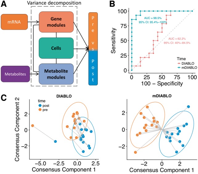
Asthma study: cross-over design and module-based analysis. (A) DIABLO design includes module-based decomposition to discriminate pre- and post-allergen challenge samples. (B) Receiver operating characteristic curves comparing standard DIABLO and multilevel DIABLO for repeated measures (mDIABLO) using leave-one-out CV. (C) Component plots of the pre- and post-challenge samples (DIABLO and mDIABLO)

We compared the standard DIABLO with a multilevel model (mDIABLO) that accounts for the repeated measures (pre/post) experimental design by isolating the within-sample variation from each of the three datasets (Fig. 4A; Supplementary Section S7; Liquet et al., 2012). Both DIABLO approaches were applied to identify a multi-omics biomarker panel consisting of cells, gene and metabolite modules that discriminated pre- from post-AIC samples on two component sets. mDIABLO outperformed DIABLO (Area Under the Receiver Operating Characteristic curve (AUC) = 98.5% versus AUC = 62.2%) with greater separation between the pre- and post-AIC samples (Fig. 4B and C). Common features (pathways) were identified across omics types in mDIABLO but not in standard DIABLO (Supplementary Fig. S17). For example, Tryptophan metabolism and Valine, leucine and isoleucine metabolism pathways were identified in both the gene and the metabolite module datasets. Groups of correlated features characterizing pre- and post-AIC samples were identified with mDIABLO (Supplementary Fig. S18). Interestingly, the Asthma pathway was identified despite individual gene members not being significantly altered post-AIC (Supplementary Fig. S19) and was negatively associated with Butanoate metabolism and positively associated with basophils, a hallmark cell-type in asthma (Supplementary Fig. S20).

4 Discussion

DIABLO aims to identify coherent patterns between datasets that change with respect to different phenotypes. This data-driven, holistic, and hypothesis-free tool can be used to derive robust biomarkers and, ultimately, improve our understanding of the molecular mechanisms that drive disease. We found that unsupervised methods identified features that formed strong interconnected multi-omics networks, but led to poor discriminative ability. In contrast, features identified by supervised methods were discriminative, but formed sparsely connected networks. The tradeoff between correlation and discrimination is a fundamental challenge when trying to identify biologically relevant biomarkers that are also clinically relevant (Wang, 2011). DIABLO achieves this tradeoff by incorporating a priori relationships between different omics data types to adequately model potential dysregulated processes between phenotypic groups. This may explain the superior biological enrichment of the DIABLO_full models in our benchmarking experiments. In contrast, biomarkers were different when we assumed no association between datasets with DIABLO_null and existing multi-step integrative strategies. Therefore, by controlling the tradeoff between correlation and discrimination, DIABLO uncovered novel multi-omics biomarkers that have not previously been identified using existing integrative strategies. These novel biomarkers were part of densely connected clusters which have prior known biological associations, further suggesting their potential biological plausibility.

DIABLO assumes a linear relationship between the selected omics features to explain the phenotypic response, an assumption that may not apply in some biological research areas, for example when integrating distance-based metagenomics studies, where kernel approaches could be further explored (Mariette and Villa-Vialaneix, 2018). Selecting the optimal number of variables requires repeated cross-validation to ensure unbiased classification error rate evaluation. A grid approach was deemed reasonable and provided very good performance results, but several iterations to refine the grid may be required depending on the complexity of the classification problem. The grid search algorithm is efficient, but we advise using a broad filtering strategy to alleviate computational time when dealing with extremely large datasets (i.e. >50 000 features each, see Rohart et al., 2017). DIABLO was primarily developed for omics-measurements on a continuous scale after normalization, and further developments are needed for categorical data types, such as genotype data. Finally, DIABLO, like other methods we benchmarked is likely to be affected by batch effects and presence of confounding variables. Therefore, we recommend exploratory analyses be carried out in each single omics dataset to assess these effects prior to integration.

Funding

This work was supported by the National Institute of Allergy and Infectious Diseases [U19AI118608 to C.P.S./S.J.T.] and the National Health and Medical Research Council [NHMRC] Career Development fellowship GNT1087415 [K.-A.L.C.].

Conflict of Interest: none declared.

References

- Aben N., et al. (2016) Tandem: a two-stage approach to maximize interpretability of drug response models based on multiple molecular data types. Bioinformatics, 32, i413–i420. [DOI] [PubMed] [Google Scholar]
- Allahyar A., De Ridder J. (2015) Feral: network-based classifier with application to breast cancer outcome prediction. Bioinformatics, 31, i311–i319. [DOI] [PMC free article] [PubMed] [Google Scholar]
- Argelaguet R., et al. (2018) Multi-omics factor analysis—a framework for unsupervised integration of multi-omics data sets. Mol. Syst. Biol., 14, e8124. [DOI] [PMC free article] [PubMed] [Google Scholar]
- Bersanelli M., et al. (2016) Methods for the integration of multi-omics data: mathematical aspects. BMC Bioinformatics, 17, S15. [DOI] [PMC free article] [PubMed] [Google Scholar]
- Chung I.-F., et al. (2016) Driverdbv2: a database for human cancer driver gene research. Nucleic Acids Res., 44, D975–D979. [DOI] [PMC free article] [PubMed] [Google Scholar]
- Cun Y., Fröhlich H. (2013) Network and data integration for biomarker signature discovery via network smoothed t-statistics. PLoS One, 8, e73074. [DOI] [PMC free article] [PubMed] [Google Scholar]
- Glass K., et al. (2013) Passing messages between biological networks to refine predicted interactions. PLoS One, 8, e64832. [DOI] [PMC free article] [PubMed] [Google Scholar]
- González I., et al. (2012) Visualising associations between paired ‘omics’ data sets. BioData Mining, 5, 19. [DOI] [PMC free article] [PubMed] [Google Scholar]
- Günther O.P., et al. (2012) A computational pipeline for the development of multi-marker bio-signature panels and ensemble classifiers. BMC Bioinformatics, 13, 326. [DOI] [PMC free article] [PubMed] [Google Scholar]
- Hamosh A., et al. (2005) Online Mendelian Inheritance in Man (OMIM), a knowledgebase of human genes and genetic disorders. Nucleic Acids Res., 33(Suppl. 1), D514–D517. [DOI] [PMC free article] [PubMed] [Google Scholar]
- Huang S., et al. (2017) More is better: recent progress in multi-omics data integration methods. Front. Genet., 8, 84. [DOI] [PMC free article] [PubMed] [Google Scholar]
- Kim D., et al. (2013) ATHENA: identifying interactions between different levels of genomic data associated with cancer clinical outcomes using grammatical evolution neural network. BioData Mining, 6, 23. [DOI] [PMC free article] [PubMed] [Google Scholar]
- Kirk P., et al. (2012) Bayesian correlated clustering to integrate multiple datasets. Bioinformatics, 28, 3290–3297. [DOI] [PMC free article] [PubMed] [Google Scholar]
- Langfelder P., Horvath S. (2008) WGCNA: an R package for weighted correlation network analysis. BMC Bioinformatics, 9, 559. [DOI] [PMC free article] [PubMed] [Google Scholar]
- Lê Cao K., et al. (2008) A sparse PLS for variable selection when integrating omics data. Stat. Appl. Genet. Mol. Biol., 7, 1–29. [DOI] [PubMed] [Google Scholar]
- Lê Cao K.-A., et al. (2011) Sparse PLS discriminant analysis: biologically relevant feature selection and graphical displays for multiclass problems. BMC Bioinformatics, 12, 253. [DOI] [PMC free article] [PubMed] [Google Scholar]
- Li W., et al. (2012) Identifying multi-layer gene regulatory modules from multi-dimensional genomic data. Bioinformatics, 28, 2458–2466. [DOI] [PMC free article] [PubMed] [Google Scholar]
- Liberzon A., et al. (2015) The molecular signatures database hallmark gene set collection. Cell Syst., 1, 417–425. [DOI] [PMC free article] [PubMed] [Google Scholar]
- Liquet B., et al. (2012) A novel approach for biomarker selection and the integration of repeated measures experiments from two assays. BMC Bioinformatics, 13, 325. [DOI] [PMC free article] [PubMed] [Google Scholar]
- Lock E.F., et al. (2013) Joint and individual variation explained (JIVE) for integrated analysis of multiple data types. Ann. Appl. Stat., 7, 523. [DOI] [PMC free article] [PubMed] [Google Scholar]
- Ma S., et al. (2016) Breast cancer prognostics using multi-omics data. AMIA Jt Summits Transl. Sci. Proc., 2016, 52. [PMC free article] [PubMed] [Google Scholar]
- Mariette J., Villa-Vialaneix N. (2018) Unsupervised multiple kernel learning for heterogeneous data integration. Bioinformatics, 34, 1009–1015. [DOI] [PubMed] [Google Scholar]
- Meng C., et al. (2016) Dimension reduction techniques for the integrative analysis of multi-omics data. Brief. Bioinform., 17, 628–641. [DOI] [PMC free article] [PubMed] [Google Scholar]
- Ritchie M.D., et al. (2015) Methods of integrating data to uncover genotype–phenotype interactions. Nat. Rev. Genet., 16, 85. [DOI] [PubMed] [Google Scholar]
- Rohart F., et al. (2017) mixOmics: an R package for ‘omics feature selection and multiple data integration. PLoS Comput. Biol., 13, e1005752. [DOI] [PMC free article] [PubMed] [Google Scholar]
- Singh A., et al. (2013) Gene-metabolite expression in blood can discriminate allergen-induced isolated early from dual asthmatic responses. PLoS ONE, 8, e67907. [DOI] [PMC free article] [PubMed] [Google Scholar]
- Singh A., et al. (2014) Th17/Treg ratio derived using DNA methylation analysis is associated with the late phase asthmatic response. Allergy Asthma Clin. Immunol., 10, 32. [DOI] [PMC free article] [PubMed] [Google Scholar]
- Sokolov A., et al. (2016) Pathway-based genomics prediction using generalized elastic net. PLoS Comput. Biol., 12, e1004790. [DOI] [PMC free article] [PubMed] [Google Scholar]
- TCGA Research Network (2012) Comprehensive molecular portraits of human breast tumours. Nature, 490, 61–70. [DOI] [PMC free article] [PubMed] [Google Scholar]
- Tenenhaus A., Tenenhaus M. (2011) Regularized generalized canonical correlation analysis. Psychometrika, 76, 257–284. [DOI] [PubMed] [Google Scholar]
- Tenenhaus A., et al. (2014) Variable selection for generalized canonical correlation analysis. Biostatistics, 15, 569–583. [DOI] [PubMed] [Google Scholar]
- Tibshirani R. (1996) Regression shrinkage and selection via the lasso. J. R. Stat. Soc. Ser. B (Methodological), 58, 267–288. [Google Scholar]
- van de Wiel M.A., et al. (2016) Better prediction by use of co-data: adaptive group-regularized ridge regression. Stat. Med., 35, 368–381. [DOI] [PubMed] [Google Scholar]
- Wang B., et al. (2014) Similarity network fusion for aggregating data types on a genomic scale. Nat. Methods, 11, 333. [DOI] [PubMed] [Google Scholar]
- Wang T.J. (2011) Assessing the role of circulating, genetic, and imaging biomarkers in cardiovascular risk prediction. Circulation, 123, 551–565. [DOI] [PMC free article] [PubMed] [Google Scholar]
- Xie B., et al. (2013) miRCancer: a microRNA–cancer association database constructed by text mining on literature. Bioinformatics, 29, 638–644. [DOI] [PubMed] [Google Scholar]
- Yugi K., et al. (2016) Trans-omics: how to reconstruct biochemical networks across multiple ‘omic’ layers. Trends Biotechnol., 34, 276–290. [DOI] [PubMed] [Google Scholar]
- Zeng I.S.L., Lumley T. (2018) Review of statistical learning methods in integrated omics studies (an integrated information science). Bioinform. Biol. Insights, 12, 117793221875929. [DOI] [PMC free article] [PubMed] [Google Scholar]
- Zhang S., et al. (2011) A novel computational framework for simultaneous integration of multiple types of genomic data to identify microRNA-gene regulatory modules. Bioinformatics, 27, i401–i409. [DOI] [PMC free article] [PubMed] [Google Scholar]
- Zhang S., et al. (2012) Discovery of multi-dimensional modules by integrative analysis of cancer genomic data. Nucleic Acids Res., 40, 9379–9391. [DOI] [PMC free article] [PubMed] [Google Scholar]
- Zhu J., et al. (2012) Stitching together multiple data dimensions reveals interacting metabolomic and transcriptomic networks that modulate cell regulation. PLoS Biol., 10, e1001301. [DOI] [PMC free article] [PubMed] [Google Scholar]
Associated Data
This section collects any data citations, data availability statements, or supplementary materials included in this article.