Inferring clonal heterogeneity in cancer using SNP arrays and whole genome sequencing

Abstract

Motivation

Clonal heterogeneity is common in many types of cancer, including chronic lymphocytic leukemia (CLL). Previous research suggests that the presence of multiple distinct cancer clones is associated with clinical outcome. Detection of clonal heterogeneity from high throughput data, such as sequencing or single nucleotide polymorphism (SNP) array data, is important for gaining a better understanding of cancer and may improve prediction of clinical outcome or response to treatment. Here, we present a new method, CloneSeeker, for inferring clinical heterogeneity from sequencing data, SNP array data, or both.

Results

We generated simulated SNP array and sequencing data and applied CloneSeeker along with two other methods. We demonstrate that CloneSeeker is more accurate than existing algorithms at determining the number of clones, distribution of cancer cells among clones, and mutation and/or copy numbers belonging to each clone. Next, we applied CloneSeeker to SNP array data from samples of 258 previously untreated CLL patients to gain a better understanding of the characteristics of CLL tumors and to elucidate the relationship between clonal heterogeneity and clinical outcome. We found that a significant majority of CLL patients appear to have multiple clones distinguished by copy number alterations alone. We also found that the presence of multiple clones corresponded with significantly worse survival among CLL patients. These findings may prove useful for improving the accuracy of prognosis and design of treatment strategies.

Availability and implementation

Code available on R-Forge: https://r-forge.r-project.org/projects/CloneSeeker/

Supplementary information

Supplementary data are available at Bioinformatics online.

1 Introduction

Chronic lymphocytic leukemia (CLL) is the most common adult form of leukemia in the United States, with approximately 20 000 new cases each year, and over 4000 deaths (American Cancer Society, 2018). Although the disease can usually be successfully treated, relapse occurs eventually in a majority of cases (Shustik et al., 2017). Patients with refractory disease are now often treated with the BTK inhibitor ibrutinib, though ibrutinib resistance has also become a problem (Ahn et al., 2017). The occurrence of multiple copy number alterations (CNAs, or CNVs) has been found to correlate with poor prognosis and relapse, and certain specific CNVs, such as 17p deletion and 11q deletion, also correspond with more aggressive disease (Nabhan et al., 2017).

Clonal heterogeneity is a common occurrence in many types of cancer, including CLL (Schuh et al., 2012). Furthermore, heterogeneity may correlate with, or even help explain, important clinical variables such as prognosis, response to treatment and chance of relapse. However, the clinical implications of clonal heterogeneity in CLL, as well as why it occurs in some patients but not others, is not fully understood. This is in part because inferring the presence of clonal heterogeneity in cancer patients with common assays (such as SNP arrays) is difficult. Tools have been developed (notably PyClone, SciClone, EXPANDS and ABSOLUTE) for inferring clonal heterogeneity from DNA sequencing data, but none of these effectively and thoroughly infers clonal heterogeneity from SNP array data alone (Andor et al., 2014; Carter et al., 2012; Miller et al., 2014; Roth et al. 2014). However, public datasets contain data from tens of thousands of SNP arrays (for example, more than 30 000 in the Gene Expression Omnibus) where clonal heterogeneity is potentially interesting.

In this paper, we propose a method called CloneSeeker that uses a Bayesian algorithm to detect clonal heterogeneity using copy number estimates derived from either SNP array data, or single nucleotide variant (SNV) information from sequencing data, or both. We begin by demonstrating our method and illustrating its effectiveness on simulated data. Next, we apply CloneSeeker to SNP array data on samples from a set of 258 previously untreated CLL patients. Of course, some clones in a tumor are likely distinguished by point mutations or other aberrations not detectable by SNP arrays. Such clones obviously will not be found if we only have SNP array data. However, given the importance of copy number alterations in CLL, it is likely that SNP arrays are capable, through our method, of elucidating many of the most important clones contributing to the heterogeneity of CLL tumors.

2 Materials and methods

Our CloneSeeker algorithm takes as input (i) a data frame with segmented SNP array data, with a row for each segment, and columns for: chromosome, segment start, segment end, log R ratio, B allele frequency (BAF) and number of markers per segment; and/or (ii) a data frame with SNV data, containing a row for each SNV, and columns for: chromosome, locus, total read count and variant allele fraction (VAF).

The output of the algorithm consists of: the number, K, of clones; a vector ψ of the tumor fraction allocated to each clone (with non-negative entries summing to one); a matrix for each clone delineating the inferred allelic copy numbers at each segment; and a matrix for each clone delineating the inferred number of mutated copies at each somatic mutation site.

2.1 Statistical model for SNP copy number data

CloneSeeker works on SNP array data by first searching for the set of integer allelic copy number values that maximizes the posterior probability, for each segment, given the number, K, of clones and a vector, ψ, indicating the fraction of cancer cells belonging to each clone. The posteriors are combined across all segments to find the best parameter set (ψ-values, copy number assignments, etc.). Specifically, the algorithm searches for the maximum a posteriori (MAP) ψ values through a simplex of possible ψ vectors allowing for between 1 and 5 possible clones. From there, the search space for ψ is narrowed and a new subspace of potential ψ-vectors is generated. The process continues for several iterations before yielding the optimal ψ-vector and matrix of subclonal, segment-wise copy number values.

The ‘raw’ SNP array data consists of the Log R Ratio (LRR) and Minor Allele Frequency (MAF) at each SNP in the SNP array. The LRR is defined as:

$$\mathit{LR}{R}_i=\mathit{Lo}{g}_{10}\left(\frac{C{N}_i}{2}\right)$$

where CN_i denotes the total copy number at locus i. The MAF is:

$${\text{MAF}}_{\mathrm{i}}={ \mathrm{B}}_{\mathrm{i}}/\left({\mathrm{A}}_{\mathrm{i}}+{ \mathrm{B}}_{\mathrm{i}}\right)$$

where A and B are the copy number for alleles A and B (where the B allele is defined as the less common or non-germline variant at a given locus), respectively. Note that CN = A + B.

Using the LRR and MAF we can estimate the number of copies of each allele (A and B) present at each SNP. Using the LRR we can back-compute the total copy number, CN. We do not, however, only use the total copy number estimate from the LRR, but also the allele fraction information (the MAF), to assess copy number alteration and multiclonality. This is because allele fraction data is informative about copy number state (e.g. an MAF value of .33 is suggestive of a gain of copy: 3 copies in total, with 1 copy belonging to the minor allele). Additionally, merely using the total copy number estimate ignores the occurrence of loss of heterozygosity, a potentially important type of CNV that may contribute to clonal heterogeneity.

Multiplying total copy number by 1– MAF and MAF (at each locus), we get estimates of the number of A and B copies, respectively, at each SNP. We call these values, denoted X and Y, the inferred copy numbers. Specifically, X and Y are computed as follows:

$$X_i=2\mathrm{*}\mathit{MA}{F}_i\mathrm{*}{10}_{}^{\mathit{LR}{R}_i}$$

$$Y_i=2\mathrm{*}\left(1-\mathit{MA}{F}_i\right)\mathrm{*}{10}_{}^{\mathit{LR}{R}_i}$$

where i now denotes the ith segment. The statistical model for X and Y (specifically, of their relationship with A and B, the true allele copy numbers) is as follows:

$$X_i={ϵ}_{\mathit{xi}}+{\sum }_{j=1}^K{\psi }_j\mathrm{*}{A}_{\mathit{ij}}$$

$$Y_i={ϵ}_{\mathit{Yi}}+{\sum }_{j=1}^K{\psi }_j\mathrm{*}{B}_{\mathit{ij}}$$

ϵ._,i here denote the error terms (assumed to be approximately normal with mean 0) for X and Y at segment i. A_{i, j} and B_{i, j} are the true allelic copy number values at segment i for clone j, and ψ_j is the fraction of cancer cells belonging to the jth clone.

It is worth noting that, for our analysis, we used data that were already segmented to make computation faster. Specifically, we used circular binary segmentation to group similar SNPs into contiguous segments (Olshen et al., 2004). Given that we are regarding the genome as a collection of independent segments, each of which consists of many SNPs, we use the median of the X and Y values for all SNPs in each segment as the segment-level estimates for X and Y, respectively. The variance of the segment X and Y estimates, of course, depends on the number of SNPs in each segment.

2.1.1. Likelihood function

We assume that the Log R Ratio, LRR, can be approximated by a normal distribution. The minor allele fraction, MAF, is probably Beta-distributed. However, as above, we use the LRR and MAF to estimate the average copy number (at each SNP) for each allele and perform our statistical modeling at this level. Specifically, we model X and Y by normal distributions. The means of the distributions at segment i are:

$$E\left(X_i\right)={\sum }_{j=1}^K{\psi }_i\mathrm{*}{A}_{\mathit{ij}}$$

$$E\left(Y_i\right)={\sum }_{j=1}^K{\psi }_i\mathrm{*}{B}_{\mathit{ij}}$$

where K is the number of clones (and j therefore is the index of the ψ value). In turn, this means that the likelihood function for a given parameter set would be:

$$P\left(X_i,Y_i\right|A_i,B_i,\psi =\mathit{Normal}\left(X_i,\mu =E\left(X_i\right),\sigma ={\sigma }_i\right)\mathrm{*}$$

$$\mathit{Normal}\left(Y_i,\mu =E\left(Y_i\right),\sigma ={\sigma }_i\right)$$

Note that the likelihood function depends on σ_i, the standard deviation of X and Y for segment i. For segment i:

$${\sigma }_i=\frac{{\sigma }_0}{\sqrt{N_i}}$$

where σ₀ is the standard deviation of the estimated X and Y values at the level of individual SNPs; we estimated this parameter using SNP array data from normal patients. The parameter N_i is the size of segment i; that is, the total number of SNPs within the segment. (The number of SNPs per segment varies considerably, from as few as 1 to as many as several thousand.) Per the central limit theorem, the standard deviation of a segment of s markers should be σ₀ divided by the square root of n.

2.1.2. Prior distributions

Prior distributions for the copy number parameters A and B are assumed to follow a geometric distribution:

$$\mathrm{P}\left(\mathrm{A}\right)=\text{Geom}(\left|1-\mathrm{A}\right|,\theta )$$

$$\mathrm{P}\left(\mathrm{B}\right)=\text{Geom}(\left|1-\mathrm{B}\right|,\theta )$$

because the most probable case is when A (or B) equals 1 (i.e. the normal case, when there is one copy of each allele). Here θ determines the decay of the probability as the number of copies deviates further from 2.

The ψ values have a distribution derived from the Jeffreys prior, which means:

$$\mathrm{P}(\psi )=\text{Dirichlet}\left(1/2, 1/2, \dots \right)$$

Lastly, K, the number of clones, has a geometric prior:

$$\mathrm{P}\left(\mathrm{K}\right)=\text{Geom}(\left|1-\mathrm{K}\right|,{\theta }_{\mathrm{K}})$$

where θ_K determines the decay of the probability as the number of clones considered increases. Our implementation uses default values for θ = 0.9 and θ_K = 0.9 based on empirical assessments of the frequency of copy number states and numbers of clones. However, the appropriate parameters determining the rates of decay are open to some interpretation; the user of the R package may vary the values if there is reason to expect the prior probability of copy number gains or losses (or of additional clones) is significantly higher or lower. In the CloneSeeker software package, users can adjust the parameters θ (theta), θ_K (ktheta) and σ₀ (sigma0), respectively, to adjust the prior probability of copy number change, number of subclones, and the variance of the raw SNP array data.

2.2 Statistical model for mutation data

The statistical model for mutation data is similar. The algorithm searches for the best (maximum posterior probability) ‘mutation model’ for each SNV given the data, for each possible ψ vector, then selects the ψ vector that maximizes the posterior probability over all SNVs. By mutation model, we mean the total number of mutated copies in each clone for a given SNV. In normal copy number cases, this normally means one (out of two possible) alleles are mutated, for example, as both alleles becoming independently mutated is highly unlikely. However, if there is a gain of copy (three in total), then there may be two mutated and one unmutated copy (or alternatively one mutated and two unmutated). The set of possible mutation models is therefore bounded by the copy number state of that region of the genome.

We use the variant allele fraction (VAF) to assess clonal heterogeneity. We regard the observed number of variant counts as the output of a binomial process in which the likelihood model for the ith SNV in the dataset is as follows:

$$P\left({\mathit{VRC}}_i,{\mathit{TRC}}_i\vee \psi ,M_{\mathit{ij}},{\mathit{CN}}_{\mathit{ij}}\right)=\mathit{Binomial}\left({\mathit{VRC}}_i,{\mathit{TRC}}_i,p\right)={\sum }_{j=1}^K\frac{{\psi }_j\mathrm{*}{M}_{\mathit{ij}}}{C{N}_{\mathit{ij}}}$$

where VRC_i and TRC_i are the observed variant and total read count at the ith SNV, respectively, ψ_j is the fraction of cancer cells belonging to the jth clone, and the parameters M_ij and CN_ij are the mutated copy number and total copy number at the ith SNV for the jth clone.

2.3 Simulations

To determine the accuracy of our algorithm for clonal detection, as well as to compare its accuracy to other algorithms, we simulated both genetically heterogeneous sequencing data, for mutations (Supplementary Fig. S1), and SNP array data, for copy number information (Supplementary Fig. S2). Since one of our aims was to examine how the accuracy is affected by characteristics of the tumor, such as the number of clones or the relative sizes of the clones present, we generated diverse simulations sets, whose characteristics are illustrated in Supplementary Figure S3. We generated three simulation sets, each with 300 simulated tumors, containing:

1. point mutations only;

2. both mutations and CNVs; and

3. CNVs only.

The third set can also be interpreted as a set of cases for which only copy number data is available. We limited the maximum number of clones in a simulated tumor to five, since the accurate deconvolution of a mixture of more than five clones is, at present, essentially impossible with either SNP array data or standard-depth sequencing data.

The simulations were created using estimates of the error structure based on real data in order to generate SNP array and/or SNV data from underlying simulated genomes. A simulated genome consisted of a set of copy number states for genomic segments (on the order of a few hundred, as is common with segmented SNP array data) and/or the mutation status of a set of SNVs. The characteristics of the simulated truth are intended to recapitulate the general features of real data.

2.3.1. Artificial mixtures

In addition to purely in silico simulations, we generated another SNP array simulation set by artificially mixing SNP array data from samples believed to be genomically homogeneous. These samples were part of the HapMap project. They are expected to be clinically normal, and therefore homogenous, although several samples show evidence of structural variation. We picked several cases that appear homogeneous and contain at least one CNV. We used these to generate 300 artificial mixtures. We again limited the maximum number of clones to five. The HapMap data used for these artificial mixtures was obtained from the Gene Expression Omnibus (accession numbers: GSE17205, GSE17206, GSE17207).

2.4 Performance metrics

The results of the algorithms are reported here using Euclidean distance metrics that measure the accuracy each algorithm’s estimated parameters. We are interested in how well each algorithm determines: (i) the number of clones, (ii) the distribution (as a fraction of the tumor) of cancer cells among the clones, (iii) the detection of CNVs in each clone and (iv) the detection of mutations in each clone. The distance metrics are:

1. The number of clones, K, where the distance between true and estimated K defined as:

   $$D_K=K–K_{\mathit{true}}$$
2. The distribution (as a fraction of the tumor) of cancer cells among the existent clones; the distance metric between true and estimated $\psi$ (j being the index of the clone) is:

   $$D_{\psi }^{}=\sqrt{\sum _{j=1}^K{\left({\psi }_{\mathit{j}}–{\psi }_{\mathit{j},\mathit{true}}\right)}^2}$$
3. The detection of CNVs in each clone; the weighted distance between the true and estimated copy numbers for clone j in segment i:

   $$D_{\mathit{CN}}=\sqrt{\sum _{i=1}^N\sum _{j=1}^K{w}_{\mathit{ij}}{\left({\mathit{CN}}_{\mathit{ij}}–{\mathit{CN}}_{\mathit{ij},\mathit{true}}\right)}^2}$$

   The weight terms, w_ij, are defined as:

   $${\mathrm{w}}_{\text{ij}}={ \mathrm{N}}_{\mathrm{i}}* {\Psi }_{\mathrm{j}}$$

   where N_i = the length of the ith segment (so an erroneous copy number inference is weighted more severely for longer segments).
4. The detection of mutations in each clone. The distance metric indicating the distance between the true and estimated number of mutated copies at each locus of a putative somatic mutations, again weighted according to the size of the clone is as follows:

   $$D_M=\sqrt{\sum _{i=1}^N\sum _{j=1}^K{w}_{\mathit{ij}}{\left({\mathit{M}}_{\mathit{ij}}–M_{\mathit{ij},\mathit{true}}\right)}^2}$$

   where i denotes the mutation and j denotes the clone. The weights w_ij are defined as for copy numbers above. However, in the case of mutations, the segment length N_i = 1 for all mutations.

We use these weighted distance metrics to avoid having to set arbitrary cutoffs for declaring an algorithm accurate or inaccurate with respect to subclonal fraction. Additionally, the use of continuous distance metrics allows for the assessment of accuracy of inferences even when the number of inferred clones is incorrect (for example, if an algorithm infers 3 clones when there are actually 4, the accuracy of what is inferred regarding CNVs or mutation can still be assessed). Lastly, this allows us to weight copy number and mutation assignment errors according to the size of the genomic segment (for CNVs) and the size of the clone (for both CNVs and mutations).

2.5 Clinical data

Samples from patients with CLL were collected at the University of Texas M.D. Anderson Cancer Center between August 17, 2000, and December 15, 2008 The SNP array data used in our analysis was generated using Illumina610Quadv1 BeadChips (Illumina Inc., San Diego, CA) on 258 previously untreated CLL patients. The method is described in greater detail in Schweighofer et al. (2013). Clinical follow-up was available for 241 patients. We conducted survival analysis on several time-to-event variables (progression free survival, time to treatment and overall survival) to determine the clinical association between the presence of clonal heterogeneity (or number of clones) and clinical outcome for these 241 CLL patients; characteristics of the patient population are shown in Table 1.

Table 1.

Characteristics of CLL patient population

	Single clone cases (with percent of total)	Multi-clone cases	Association with multiclonality
Race			P = 0.2 (χ2 = 3.2)
Black	4 (1.66)	7 (2.9)
Hispanic	2 (0.83)	4 (1.66)
White	129 (53.53)	95 (39.42)
Sex			P = 0.338 (χ2 = 0.917)
Female	37 (15.35)	36 (14.94)
Male	98 (40.66)	70 (29.05)
Mutation Status			P = 0.178 (χ2 = 1.82)
Mutated	63 (26.14)	39 (16.18)
Unmutated	72 (29.88)	66 (27.39)
Rai Stage			P = 0.009 (χ2 = 13.65)
0	7 (2.9)	15 (6.22)
1	51 (21.16)	43 (17.84)
2	44 (18.26)	31 (12.86)
3	10 (4.15)	12 (4.98)
4	22 (9.13)	4 (1.66)
Zap70 Expression			P = 0.184 (χ2 = 1.77)
Negative	63 (26.14)	42 (17.43)
Positive	54 (22.41)	54 (22.41)
Dohner Category			P = 0.006 (χ2 = 14.3)
Del11q	15 (6.22)	19 (7.88)
Del13q	52 (21.58)	35 (14.52)
Del17p	4 (1.66)	8 (3.32)
Normal	48 (19.92)	21 (8.71)
Tri12	15 (6.22)	23 (9.54)
Age at diagnosis	54.55*	59.58	P = 0.001 (t = 3.35)
Time (from sample) to treatment	33.3*	30.3*	P = 0.16 (logrank = 2.02)

2.6 Software

Our analysis was performed using R version 3.4.0, and the code used, which we have developed into an R-package, is available on R-forge. For our survival analysis we used the ‘survival’ (version 2.41-3) and ‘prodlim’ (version 1.6.1) packages.

3 Results

3.1 Selecting other algorithms for comparison

In order to select other clonal heterogeneity algorithms to compare with ours, we reviewed the characteristics of existing algorithms, focusing on required inputs, optional inputs, kinds of outputs and code availability (Table 2). A host of such algorithms exist, including PyClone, SciClone, EXPANDs and ABSOLUTE. We looked for algorithms that yielded comparable results amenable to comparison. Specifically, we required tools that (i) attempted to deconvolute the cancer cell population into distinct clones (as opposed to merely giving estimates of the fraction of cells containing each detected subclonal alteration, as some tools do), (ii) did not require single cell sequencing data, and (iii) had publicly available source code. Table 2 describes various clonal heterogeneity-related tools, their features, and whether or not (and why) they were excluded from our comparative analysis. Algorithms were excluded for a number of reasons, such as only inferring alteration allele fractions but not the number of distinct clones, or requiring paired normal data. Additionally, we preferred algorithms that accepted copy number alteration data, as CNVs are an important source of clonal heterogeneity in many cancers. This led to our final selection of SciClone and Expands for comparison with CloneSeeker.

Table 2.

Properties of clonal heterogeneity tools, including possible and required input and output

Name	Language	Seq. data	WES	SNP Array	Alt. frac.	Clonal frac.	No. clones	Mutation Assignments	CNV Assignments
		Input:			Output:
CloneSeeker	R	Optional	Optional	Optional	Yes	Yes	Yes	Yes	Yes
EXPANDS	R	Required*	Optional	Optional	Yes	Yes	Yes	Yes	Yes
SciClone	R	Required*	Optional	Optional	Yes	Yes	Yes	Yes	Yes
PyClone	Python	Required*	Optional	Optional	Yes	No	Yes	Yes	Yes
ABSOLUTE	R	Required*	Optional	Optional	Yes	No	No	No	No
Gaucho	R	Required*	Optional	No	Yes	Yes	Yes	Yes	No
TitanCNA	R	Required	No	No	Yes	No	No	No	No
PurBayes	R	Required*	Optional	No	No	Yes	Yes	No	No
QuantumClone	R	Required*	Optional	No	Yes	Yes	Yes	Yes	No
CHAT	R	Optional	Optional	Optional	Yes	Yes	Yes	Yes	No
FACETS	R	Required*	Optional	No	Yes	Yes	Yes	No	Yes

Note: Entries bolded indicate reasons for exclusion from our comparative analysis. *Seq. data means some form of sequencing data, either whole genome or exome. (Andor et al. 2013; Carter et al. 2012; Ha et al., 2014; Larson and Fridley, 2013; Li and Li, 2014; Melchor et al. 2014; Miller et al. 2014; Roth et al. 2014; Shen and Seshan, 2016).

3.2 Analysis of simulated data

We applied CloneSeeker, Expands and SciClone to simulated datasets 1 (mutation only) and 2 (both mutations and CNVs). CloneSeeker inferred the number of clones, the distribution of cancer cells among the clones and the copy number and mutation assignments more accurately in both simulation sets than the other two algorithms (Figs 1 and 2). It is worth noting that all three algorithms were fairly consistent with each other in the assignment of mutations to clones.

Fig. 1.

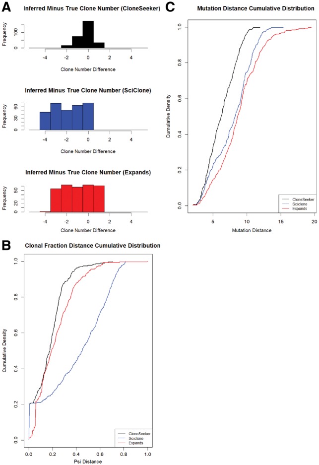
Comparative performance of each method on simulations with mutations only. (A) Histograms of the difference between true and inferred number of clones for each algorithm. (B) Cumulative distribution of the distance between the true and inferred clonal fractions. (C) Cumulative distribution of the weighted mutation-distance

Fig. 2.

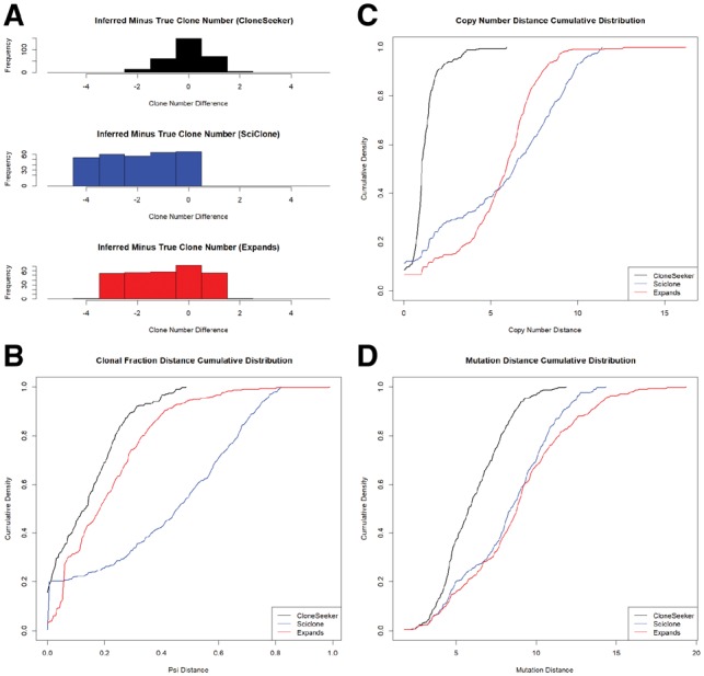
Comparative performance of each method on simulations with both mutations and CNVs). (A) Histograms of differences between true and inferred copy number. (B) Cumulative distributions of distances between true and inferred clonal fractions. (C) Cumulative distributions of distances between true and inferred copy numbers. (D) Distributions of distances between true and inferred mutation copy numbers

There are reasons to expect (as we observe) that SciClone would do poorly in copy number analysis. Specifically, SciClone assumes homogeneity in copy number, so cases where subclonal copy number alterations distinguish cancer cell subpopulations will tend to confound the SciClone algorithm. Expands and CloneSeeker handle such cases better. Additionally, SciClone assigns every mutation to a single cluster (clone), with the tumor fractions of clones summing to 1, while Expands and CloneSeeker both allow a given mutation (or CNV) to be assigned to multiple clones, which would presumably be distinguished from each other by a different alteration (suggesting that one of the clones may be a descendant of the other). Expands also infers the ‘family tree’ describing the genealogical relationships between the difference clones.

In all simulation sets, as expected, the accuracy of each algorithm declines as the number of clones increases. SNP array data (and sequencing data with standard read depth) is generally unable to deconvolute a population of more than five clones. There are two major reasons for this. Firstly, as the number of clones increases, the clonal fractions get smaller, which makes them less detectable. A clone that makes up less than 5% of the cancer cell fraction will be difficult to discern from noise. Secondly, the subclonal fractions tend to get closer together as the number of clones increases, which makes them more difficult to resolve; e.g. it is more difficult to resolve two different clones making up 10% and 11% of a tumor than two clones making up 40 and 50% of a tumor.

In Figure 3A–C, we show the result of our analysis on simulated copy number data (just copy number alterations, no mutations). This simulation set is most relevant to our later analysis of CLL data. Since the algorithms to which we are comparing CloneSeeker require sequencing data of some kind as input, we cannot make such comparisons for this set. However, we can observe that CloneSeeker identifies the correct number of clones exactly about 60% of the time, and is within one about 90% of the time.

Fig. 3.

CloneSeeker performance on simulations with CNV only. The panels on the left are performance metrics for CloneSeeker’s results on simulated data with no point mutations; those on the right are metrics for the results from artificial mixtures of HapMap samples. (A and D) are histograms of the difference between the true and inferred number of clones; (B and E) are cumulative distributions for the distance between true and inferred clonal fractions; and (C and F) are distributions of the weighted copy number distances

3.3 Artificial mixtures

Next, we applied CloneSeeker to our artificial mixture set. Because both Expands and SciClone require mutation data, we cannot apply these for comparison. The results of this analysis are shown in Figure 3D–F. This simulation set, generated by mixing normal HapMap sample data after adding CNVs to simulate heterogeneity, demonstrates that our algorithm performs reasonably well on simulated data in which the error structure recapitulates that of actual SNP array data.

3.4 CLL Analysis

We applied CloneSeeker to 258 CLL patient samples in order to assess the clonal architecture of their tumors. The characteristics inferred are summarized in Supplementary Figure S4. Using our algorithm, about 44% of CLL patients (106 out of 241) have multiple cancer clones. Though a significant number (17) have 3 clones, none have 4 or more detectable clones. The fraction of the genome altered also tends to rise steadily with the number of clones.

Using the subset of 241 patients for whom clinical data were available, we performed statistical analyses to test the association between multi-clonality and common clinical and demographic features (Table 1). We found that the presence of multiple clones was significantly associated with several variables, including Rai stage (P = 0.009), Döhner cytogenetic category (P = 0.006) and age at diagnosis (P = 0.001). Döhner categories known to be associated with worse prognosis made up larger fractions of cases with multiple clones (del17p, 7.5% of multi-clone versus 3.0% of single clone; del11q, 17.9% versus 11.2%) while Döhner categories with relatively good prognosis, del13q, made up larger fractions of single clone cases (33.0% of multi-clone versus 38.8% of single clone). Patients with normal karyotype, corresponding to intermediate prognosis, were disproportionally single clone cases (19.8% of multi-clone versus 35.6% of single clone); Trisomy 12, which also has an intermediate prognosis, was 21.7% of multi-clone versus 11.2% of single-clone (Döhner et al., 2000).

3.4.1. Karyotype analysis

We also looked at the number of clones observed in karyotype data from 4254 CLL patient samples (Supplementary Fig. S5) collected and processed at OSU Wexner Medical Center. We used CytoGPS to parse the karyotype data and determine the number of subclones per patient. (Abrams et al., 2015; Abrams, 2016) We observed that, in these patients, a sizable majority (74%) had more than one clone apparent, significantly more than observed in our SNP array data. Many of the patients karyotyped, it is worth noting, have been treated and have refractory disease, while all of those in our SNP array data analysis were untreated, so the higher rate of multiclonality in the karyotype data may be related to the effects of treatment.

3.4.2. Survival analysis

We also conducted survival analysis to determine if the presence of multiple cancer clones was associated with clinical outcome. We found that clinical outcome was worse for patients with multiple subclones. This relationship is apparent for overall survival from time of sample collection, overall survival after treatment, time to treatment and time to progression (Fig. 4 and Supplementary Fig. S6); it is, however, only statistically significant for overall survival after sample (P = 0.012) and after treatment (P = 0.0017). We also performed survival analyses including complex karyotype (defined, as usual, as having three or more distinct CNVs; it serves here as a measure for overall genomic instability) as an independent variable (Supplementary Fig. S7). We found that even when accounting for complex karyotype as a potential confounder, there was a statistically significant independent association between the presence of multiple clones and overall survival both after sample (P = 0.0314) and after treatment (P = 0.0059).

Fig. 4.

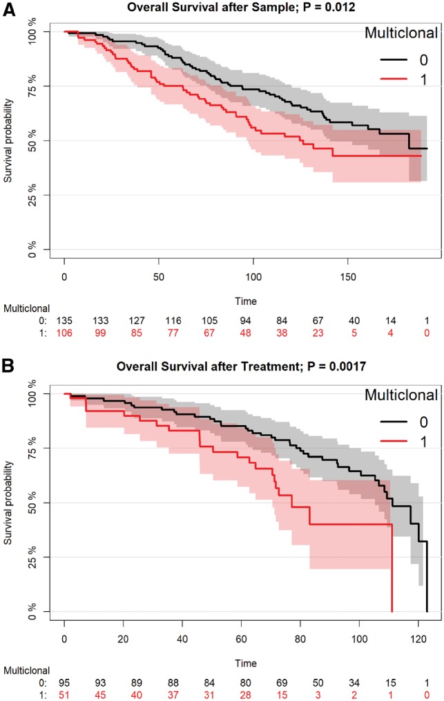
Survival analysis using Cox proportional hazard model on CLL patient data. A) Overall survival after sampling as a function of multiclonality (n = 241). B) Overall survival after treatment as a function of multiclonality (n = 146)

4 Discussion

Clonal heterogeneity is an important characteristic of many cancers, including CLL. It is believed to potentially influence clinical outcome and may play a role in disease progression and evolution of resistance to treatment. Genetically distinct clones may also respond differently to different types of treatment, and may exhibit differential growth rates or heterogeneity in other traits. To date, however, most tools developed to infer the presence (or absence) of clonal heterogeneity in tumors have focused on point mutations. Being able to effectively discern heterogeneity in both point mutations and structural variation, however, is necessary to fully assess how diverse tumor cell populations are, especially in CLL, which is known to often harbor CNVs, and for which several common CNVs are important biomarkers.

We presented an algorithm here, named CloneSeeker, which has proven generally more effective at accurately inferring the clonal architecture than two other commonly used algorithms, using either sequencing data, SNP array data, or both. We demonstrated this using multiple sets of simulations. When we applied CloneSeeker to CLL data, we found (in accordance with some prior studies) that, even in untreated patients, clonal heterogeneity is a common occurrence in CLL, affecting almost half of the patients in our dataset. No cases had more than three clones, though it is worth noting that this observation may be an artifact of the fact that cases with many clones are likely to have smaller clones, and the smaller a clone, the harder it is to detect; clones making up less than 5% of the cancer cell population, for example, are often undetectable with standard SNP array data or whole genome sequencing data.

The next important step in analysis of clonal heterogeneity would be to determine the clinical implications of clonal heterogeneity in CLL. Some researchers have associated clonal heterogeneity with disease progression and drug resistance. If a tumor consists of many distinct clones, for example, regardless of the initial clinical state of the disease, it may be more likely that one of the clones will eventually undergo rapid expansion and cause disease progression, or develop a mutation conferring drug resistance (Burgery et al., 2016; Landau et al., 2015). Of course, it is difficult to separate the effects of clonal heterogeneity itself and concomitant Darwinian inter-clonal competition from other potentially confounding factors, such as overall mutation rate (which one may expect to correlate with multiclonality). Additionally, treatment itself may induce subclonal mutations, which adds to the complications of determining the direction of causality in the association between clonal heterogeneity and disease progression or treatment resistance (Szikriszt et al., 2016).

Finally, we performed survival analysis using Cox proportional hazard models to assess the relationship between clonal heterogeneity and clinical outcome. We found that the presence of more than one clone corresponds with worse survival in all clinical outcome related variables tested, and the relationship is statistically significant for two variables: overall survival after sample and overall survival after treatment. This is in accordance with other studies indicating a relationship between clonal heterogeneity and clinical outcome. Additionally, we verified that, even after accounting for general genomic instability by including presence or absence of complex karyotype in the survival analysis, multiclonality is still independently associated with poorer survival.

In future research, we will seek to determine the relationship between the fraction of cells possessing particular CNVs and clinical outcome.

References

- Andor N. et al. (2013) EXPANDS: expanding ploidy and allele frequency on nested subpopulations. Bioinformatics, 30, 50–60. [DOI] [PMC free article] [PubMed] [Google Scholar]
- Abrams Z.B. (2016) A Translational Bioinformatics Approach to Parsing and Mapping ISCN Karyotypes: a Computational Cytogenetic Analysis of Chronic Lymphocytic Leukemia (CLL). Doctor of Philosophy, Ohio State University, Integrated Biomedical Science Graduate Program.
- Abrams Z.B. et al. (2015) Text mining and data modeling of karyotypes to aid in drug repurposing efforts. Stud. Health Technol. Inf., 216, 1037.. [PMC free article] [PubMed] [Google Scholar]
- Ahn I.E. et al. (2017) Clonal evolution leading to ibrutinib resistance in chronic lymphocytic leukemia. Blood, 6, 719294. [DOI] [PMC free article] [PubMed] [Google Scholar]
- American Cancer Society. (2018) Key Statistics for Chronic Lymphocytic Leukemia. American Cancer Society, Atlanta, GA. [Google Scholar]
- Andor N. et al. (2014) EXPANDS: expanding ploidy and allele frequency on nested subpopulations. Bioinformatics, 30, 50–60. [DOI] [PMC free article] [PubMed] [Google Scholar]
- Burger J.A. et al. (2016) Clonal evolution in patients with chronic lymphocytic leukaemia developing resistance to BTK inhibition. Nat. Commun., 7, 11589. [DOI] [PMC free article] [PubMed] [Google Scholar]
- Carter S.L. et al. (2012) Absolute quantification of somatic DNA alterations in human cancer. Nat. Biotechnol., 30, 413–421. [DOI] [PMC free article] [PubMed] [Google Scholar]
- Döhner H. et al. (2000) Genomic aberrations and survival in chronic lymphocytic leukemia. N. Engl. J. Med., 343, 1910–1916. [DOI] [PubMed] [Google Scholar]
- Ha G. et al. (2014) TITAN: inference of copy number architectures in clonal cell populations from tumor whole-genome sequence data. Genome Res., 24, 1881–1893. [DOI] [PMC free article] [PubMed] [Google Scholar]
- Landau D.A. et al. (2015) Mutations driving CLL and their evolution in progression and relapse. Nature, 526, 525–530. [DOI] [PMC free article] [PubMed] [Google Scholar]
- Larson N.B., Fridley B.L. (2013) PurBayes: estimating tumor cellularity and subclonality in next-generation sequencing data. Bioinformatics, 29, 1888–1889. [DOI] [PMC free article] [PubMed] [Google Scholar]
- Li B., Li J.Z. (2014) A general framework for analyzing tumor subclonality using SNP array and DNA sequencing data. Genome Biol., 15, 473.. [DOI] [PMC free article] [PubMed] [Google Scholar]
- Nabhan C. et al. (2017) Clonal evolution leading to ibrutinib resistance in chronic lymphocytic leukemia. Blood, 6, 719294. [DOI] [PMC free article] [PubMed] [Google Scholar]
- Miller C.A. et al. (2014) SciClone: inferring clonal architecture and tracking the spatial and temporal patterns of tumor evolution. PLoS Comput. Biol., 10, e1003665.. [DOI] [PMC free article] [PubMed] [Google Scholar]
- Melchor L. et al. (2014) Single-cell genetic analysis reveals the composition of initiating clones and phylogenetic patterns of branching and parallel evolution in myeloma. Leukemia, 28, 1705–1715. [DOI] [PubMed] [Google Scholar]
- Olshen A.B. et al. (2004) Circular binary segmentation for the analysis of array-based DNA copy number data. Biostatistics, 5, 557–572. [DOI] [PubMed] [Google Scholar]
- Roth A. et al. (2014) PyClone: statistical inference of clonal population structure in cancer. Nat. Methods, 11, 396–398. [DOI] [PMC free article] [PubMed] [Google Scholar]
- Schuh A. et al. (2012) Monitoring chronic lymphocytic leukemia progression by whole genome sequencing reveals heterogeneous clonal evolution patterns. Blood. 120, 4191–4196. [DOI] [PubMed] [Google Scholar]
- Schweighofer C.D. et al. (2013) Genomic variation by whole-genome SNP mapping arrays predicts time-to-event outcome in patients with chronic lymphocytic leukemia: a comparison of CLL and HapMap genotypes. J. Mol. Diagn. JMD, 15, 196–209. [DOI] [PMC free article] [PubMed] [Google Scholar]
- Shen R., Seshan V. (2016) FACETS: allele-specific copy number and clonal heterogeneity analysis tool for high-throughput DNA sequencing. Nucleic Acids Res., 44, e131. [DOI] [PMC free article] [PubMed] [Google Scholar]
- Shustik C. et al. (2017) Advances in the treatment of relapsed/refractory chronic lymphocytic leukemia. Ann. Hematol., 96, 1185–1196. [DOI] [PMC free article] [PubMed] [Google Scholar]
- Szikriszt B. et al. (2016) A comprehensive survey of the mutagenic impact of common cancer cytotoxics. Genome Biol., 17, 99.. [DOI] [PMC free article] [PubMed] [Google Scholar]
Associated Data
This section collects any data citations, data availability statements, or supplementary materials included in this article.