

Abstract
An important goal for psychological science is developing methods to characterize relationships between variables. Customary approaches use structural equation models to connect latent factors to a number of observed measurements, or test causal hypotheses between observed variables. More recently, regularized partial correlation networks have been proposed as an alternative approach for characterizing relationships among variables through covariances in the precision matrix. While the graphical lasso (glasso) has emerged as the default network estimation method, it was optimized in fields outside of psychology with very different needs, such as high dimensional data where the number of variables (p) exceeds the number of observations (n). In this paper, we describe the glasso method in the context of the fields where it was developed, and then we demonstrate that the advantages of regularization diminish in settings where psychological networks are often fitted (p ≪ n). We first show that improved properties of the precision matrix, such as eigenvalue estimation, and predictive accuracy with cross-validation are not always appreciable. We then introduce non-regularized methods based on multiple regression and a non-parametric bootstrap strategy, after which we characterize performance with extensive simulations. Our results demonstrate that the non-regularized methods can be used to reduce the false positive rate, compared to glasso, and they appear to provide consistent performance across sparsity levels, sample composition (p/n), and partial correlation size. We end by reviewing recent findings in the statistics literature that suggest alternative methods often have superior performance than glasso, as well as suggesting areas for future research in psychology. The non-regularized methods have been implemented in the R package GGMnonreg.
Keywords: network models, partial correlation, non-regularized, multiple regression, model selection, ℓ1-regularization
Introduction
An important goal for psychological science is to characterize the structure of associations among variables that relate to psychological constructs. A common approach is to use latent variable analysis (e.g., confirmatory factor analysis, latent class analysis, item response theory) to relate a set of observed variables to a shared underlying latent variable. More recently, proponents of a “network approach” to psychological constructs have argued that the latent variable framework ignores direct causal or functional associations among observed variables (Borsboom & Cramer, 2013). For example, a latent variable model of depression cannot account for the fact that lack of sleep leads directly to fatigue (Cramer & Borsboom, 2015), and a latent variable model of quality of life cannot account for the necessary link between being unable to walk up one flight of stairs and being unable to walk up several flights of stairs (Kossakowski et al., 2016). In response to these criticisms, researchers are increasingly employing network models in an attempt to capture these direct associations among observed variables (Epskamp & Fried, 2016). The goal of network modeling of psychological constructs is to understand constructs as a system of direct interactions among observable variables, instead of as underlying, unobservable variables.
Network models are a general class of models that can estimate any sort of association among variables (e.g., marginal or conditional associations) on many different sorts of data assuming the cases are independent (e.g., cross-sectional data, single-person longitudinal data, or a mix). Here, our focus is on the most popular type of network that has been employed in psychology, namely partial-correlation networks estimated on cross-sectional data. These models seek to estimate a sparse network of conditional relations (i.e., direct effects) among a set of observed variables measured at a single time point in a sample of people. This is accomplished by identifying non-zero off-diagonal elements of the inverse-covariance matrix of the data (i.e., the precision matrix; Dempster, 1972). When the precision matrix is standardized and the sign reversed, elements of the matrix are partial correlations that imply pairwise dependencies in which the effects of all other observed variables have been controlled for (Peng, Wang, Zhou, & Zhu, 2009). That is, a non-zero network “edge” represents a direct association between a pair of observed variables that cannot be explained by any other variables in the model. Since direct effects are often sought after in psychology, there has been an explosion of interest in network models in both methodological and applied contexts. Network models have been used to provide an alternative perspective on a wide range of constructs, including political attitudes (Dalege, Borsboom, van Harreveld, & van der Maas, 2017), psychosis (Isvoranu et al., 2017; van Rooijen et al., 2017), post-traumatic stress disorder (Armour, Fried, Deserno, Tsai, & Pietrzak, 2017; McNally et al., 2015), substance abuse (Rhemtulla et al., 2016), and well-being (Deserno, Borsboom, Begeer, & Geurts, 2017).
A wide range of methods have been proposed to estimate network model parameters (Kuismin & Sillanpää, 2017). These methods generally use some form of regularization (i.e., shrinkage) to estimate the precision matrix (Θ). In high-dimensional settings, where the number of variables (p) approaches or exceeds the number of observations (n), regularization makes estimation of an under-identified model possible. The most common type of regularization applied to network models is ℓ1-regularization (a.k.a., “least absolute shrinkage and selection operator”, or “lasso”), which adds a penalty to the estimation function that is based on the sum of the absolute values of the edges. The effect of this penalty is to push smaller estimates to exactly zero. Though psychological data are rarely high-dimensional, by pushing small edges to zero, ℓ1-regularization confers the additional benefit of producing a sparse network. From the theoretical network perspective, a system of direct effects among observed variables would not allow for determining the conditional independence structure of psychological constructs if it were fully connected (i.e., if every node were connected to every other node); thus, identifying zeros is an important theoretical goal of network modeling. Compared to customary methods (e.g., ordinary least squares) regularization procedures involve additional steps for estimation, in which developing methods that are both accurate and computationally efficient is an active area of research (Kuismin & Sillanpää, 2017). However, in psychology, the dominant estimation procedure is the graphical lasso (Friedman, Hastie, & Tibshirani, 2008), described below (Section: Precision Matrix Estimation), in which the tuning parameter (λ) is selected according to the extended Bayesian Information Criterion (EBIC; Chen & Chen, 2008). We refer to the combination of graphical lasso and EBIC-based tuning parameter selection as glassoEBIC (Foygel & Drton, 2010).
Despite the popularity of glassoEBIC in psychology, there has not been any work comparing it to alternative methods for estimating networks of psychological variables. This is problematic for two reasons. First, outside of psychology, there are several methods that have been shown to outperform glasso (Ha & Sun, 2014; Peng et al., 2009; Van Wieringen & Peeters, 2016). Compared to three alternative methods, for example, Williams, Piironen, Vehtari, and Rast (2018) recently showed that glassoEBIC rarely had the best performance with respect to identifying true non-zero covariances. Further, even with alternative methods for selecting λ (e.g., cross-validation rather than EBIC), the performance of glasso does not necessarily warrant being the default approach in psychological applications (Kuismin & Sillanpää, 2016; Mohammadi & Wit, 2015a). Second, and importantly, statistical methods to estimate network models were developed to overcome the very specific challenge of high dimensionality (Kuismin & Sillanpää, 2017). Under these conditions, the maximum likelihood estimator becomes unstable or cannot be computed altogether, thus requiring some form of regularization. Although these kinds of data structures are common in fields such as genomics (Y. R. Wang & Huang, 2014), they are the exception in psychology. Indeed, the majority of network models fitted in psychology are in low-dimensional settings (p ≪ n) (McNally et al., 2015; Rhemtulla et al., 2016; Spiller et al., 2017).
Compared to other model selection procedures, glasso may carry some distinct disadvantages. First, as a fully automated procedure, inferences about specific edges are non-trivial and require additional steps after model selection (K. Liu, Markovic, & Tibshirani, 2017; Wasserman & Roeder, 2009). This general critique applies to all automated procedures (e.g., backwards elimination), but there are additional challenges for glasso that often require debiasing–unregularizing–the estimates (Javanmard & Montanari, 2015). Second, regularization approaches are also not common in psychology (McNeish, 2015), and applied researchers may not be familiar with how inference based on such approaches differs from those of non-regularized approaches, or of the speed with which the regularization literature is evolving (Avagyan, Alonso, & Nogales, 2017; Tibshirani, 2011; Zou & Hastie, 2005). The novelty of regularization methods in psychology may give the false impression that they are necessarily superior to more common approaches for automated variable selection such as stepwise regression approaches (Henderson & Denison, 1989). In fact, in the context of network estimation, method performance is often evaluated in situations that are uncommon in psychology. For example, in Bühlmann and Van De Geer (2011), it was shown ℓ1-regularization was consistent for model selection when the number of variables (p) grew exponentially. In psychology, a more realistic situation would fix the number of variables, for example the number of items in a questionnaire, and then allow the sample size (n) to increase. Here more common approaches such as best subset selection with the standard Bayesian information criterion (BIC) are generally consistent for selecting the true model (Casella, Girón, Martinez, & Moreno, 2009; P. Zhao & Yu, 2006). Given that network models were popularized and estimation techniques optimized in fields outside of psychology with very different needs, it is important to investigate the quality of estimation methods for situations that are most common in psychological research.
The aim of the present work is to investigate the properties of the glassoEBIC procedure compared to non-regularized methods that can be used in low-dimensional settings (p < n). We thus determine whether regularization offers distinct advantages compared to model selection methods more familiar to psychologists. In the next sections, we first discuss precision matrix estimation in the context of high-dimensional settings, which are common in areas such as functional neuroimaging (Das et al., 2017), but rare in personality or clinical fields. We then introduce two non-regularized approaches, that include multiple regression and a non-parametric bootstrap strategy, for estimating networks. These approaches are novel in the context of estimating network models. In this section, we also describe the relationship between multiple regression and the precision matrix. Then, in two simulation studies, we characterize the performance of each method under conditions that are common in psychological data. We end with recommendations for both applied and methodologically oriented researchers.
Precision Matrix Estimation
The covariance matrix (Σ) plays an essential role in parametric analyses, particularly in multivariate settings such as structural equation and network modeling. In particular, network models require the inverse of the covariance matrix, called the precision matrix (Θ), to obtain partial correlations ρij as
| (1) |
which corresponds to the following elements within the precision matrix
| (2) |
In words, the partial correlations are computed by standardizing the off-diagonal elements of precision matrix and reversing the sign (±). This is analogous to obtaining bi-variate correlations from Σ, but with the additional step of sign reversal. Although this appears straightforward, Equation 2 indicates that estimating partial correlations requires inverting the sample covariance matrix Σ. Typically, Σ is estimated via maximum likelihood (ML) but this approach yields reliable estimates only under ideal conditions (Ledoit & Wolf, 2004b; Won, Lim, & Kim, 2009). For example, Kuismin and Sillanpää (2016) demonstrated that ML-estimator of the eigenvalues can be non-optimal, which then magnifies the estimation error when the covariance matrix is inverted (Ledoit & Wolf, 2004b). This can be seen in Equation 17, where the eigenvalues (i.e., D) play a critical role in inverting Σ. In particular, when the ratio of variables p to observations n (p/n) approaches one (Wong, Carter, & Kohn, 2003), it becomes difficult to reliably estimate the covariances. Furthermore, in high dimensional (n < p) settings, the ML-estimate cannot be computed due to singularity: det(Σ) = 0. That is, since the determinant equals the product of the eigenvalues and the maximum number of non-zero eigenvalues is min(n, p) (Kuismin & Sillanpää, 2017), inverting the covariance matrix is not possible (Hartlap, Simon, & Schneider, 2007). This is known as the “large p and small n” problem (Kuismin, Kemppainen, & Sillanpää, 2017) and remains a central challenge in the field of statistics (Kuismin & Sillanpää, 2016).
ℓ1-Regularization
To overcome the “large p and small n” problem, several regularization approaches have been developed to make estimation possible when Σ is non-invertible. In the familiar context of multiple regression, regularized estimation approaches estimate the ordinary least squares solution, but do so with an added penalty. Different types of regularization use different penalties: lasso uses the ℓ1-norm to find coefficients that minimize
| (3) |
In this equation, λ is the “tuning parameter”, which determines the extent to which the penalty affects the estimates. When λ = 0, no penalty is imposed and the resulting estimates are equal to the ordinary least squares estimates. When a very high value of lambda is chosen, all the estimates will be pushed to zero (H. Liu, Roeder, & Wasserman, 2010). Thus, some criterion is needed to choose the value of λ such as predictive accuracy determined with cross-validation or an information criteria (e.g., BIC; Chand, 2012). Other regularization options are to minimize the ℓ2-norm (a.k.a., “ridge” regularization, which penalizes the sum of squared estimates, resulting in smaller estimates but typically none that are exactly zero) or to minimize a combination of the ℓ1 and ℓ2 norms (a.k.a., “elastic-net”; (Zou & Hastie, 2005). Assuming the residuals are normally distributed,, minimizing the ordinary least squares estimate is equivalent to maximizing the likelihood, or in this case the penalized maximum likelihood. Importantly, by reducing coefficients to exactly zero, lasso regularization has built-in model and variable selection. For this reason, the lasso method has become popular for both regression and for estimating network models.
Extended to multivariate settings, the penalized likelihood for the precision matrix is defined as
| (4) |
where Σ is the sample covariance matrix and λp a penalty function (Gao, Pu, Wu, & Xu, 2009). The glasso method applies a penalty on the sum of absolute covariance values λp(|Θi,j|) (Friedman et al., 2008). The performance of the glasso method is strongly influenced by the choice of λ, which can be made in at least four ways: (1) choose λ that minimizes the EBIC (Foygel & Drton, 2010); (2) choose λ that minimizes the Rotation Information Criterion (RIC) (T. Zhao, Liu, Roeder, Lafferty, & Wasserman, 2012); (3) choose λ that maximizes the stability of the solution across subsamples of the data (i.e., Stability Approach to Regularization Selection; StARS) (H. Liu et al., 2010); and (4) k-fold cross-validation (Bien & Tibshirani, 2011). Interestingly, these methods can produce vastly different networks (Kuismin & Sillanpää, 2017). While a method would ideally be selected with a particular goal in mind, or based on performance in simulations that are representative of the particular field, the default method in psychology is currently EBIC
| (5) |
where l(Θ) is defined in Equation 4, E is the size of the edge set (i.e., the number of non-zero elements of Θ), and γ ∈ [0, 1] is the EBIC hyperparameter that puts an extra penalty on the size of the model space. As described in Chen and Chen (2008), there is a Bayesian justification for γ that corresponds to a prior distribution on the model space, thus providing the reason it is bounded between 0 and 1. Notably, EBIC reduces to the Bayesian Information Criterion (BIC) when γ = 0, where each model size has been assigned an equal prior probability. The selected network then minimizes EBIC with respect to λ. This is typically accomplished by assessing a large number (e.g., 100) of values of λ and selecting the one for which EBIC is smallest. There is no automatic selection procedure for the EBIC hyperparameter, but 0.5 was recommended in Foygel and Drton (2010) and Epskamp and Fried (2016). The latter further suggested that researchers who prefer to err on the side of discovery (i.e., those who prefer to find more edges, including possibly false ones) choose a γ value closer to 0, and those who prefer a more conservative approach choose a value closer to 0.5 (Epskamp & Fried, 2016).
Extensions to Psychology
Psychological applications of network modeling have widely adopted ℓ1-regularization as the default statistical approach for estimation.. However, outside of neuroscience related inquiries, there are typically far more observations (n) than variables (p) in psychological networks. In other words, the “large p and small n” (Section: ℓ1-Regularization) is not often encountered. As such, regularization is not usually necessary to produce an estimate of Θ. Further, findings from simulation studies (e.g. Mohammadi & Wit, 2015a) indicate that RIC and StARS show superior performance in terms of F1-scores1 across a number of conditions in low dimensional settings. Second, while psychological inferences are typically aimed towards explanation rather than prediction (Yarkoni & Westfall, 2017), ℓ1-regularization is known for reduced prediction error rather than accuracy of parameter estimates. Further, inference regarding the non-zero (or zero) estimates is not straightforward, as valid standard errors are not easily obtained (Hastie, Tibshirani, & Friedman, 2008). Making inference entails corrections for model selection bias (Efron, 2014; Hastie, Tibshirani, & Wainwright, 2015; Leeb, Pötscher, & Ewald, 2015), and non-traditional bootstrap schemes are often needed to achieve nominal frequentist properties (Bühlmann, Kalisch, & Meier, 2014; Chatterjee & Lahiri, 2011). In the context of network models in particular (Janková & van de Geer, 2017), statistical inference for Θ is an emerging area of research that often requires desparsifying the regularized estimates to compute confidence intervals (Janková & van de Geer, 2015; Ren, Sun, Zhang, & Zhou, 2015) and p-values (W. Liu, 2013; T. Wang et al., 2016).
Motivating Examples
In this section, we provide two motivating examples for this work that focus exclusively on precision matrix estimation. Most of the statistical literature has focused on high-dimensional settings, or situation where p approaches n, which stands in contrast to the most common psychological applications. We conducted two brief simulations to examine the performance of glassoEBIC compared to maximum likelihood estimation (MLE) in low-dimensional settings. The first motivating example assessed eigenvalue recovery, that is directly related to the accuracy with which Θ has been estimated. In particular, a “well-conditioned” covariance matrix is such that the range of eigenvalues is not too large (Schäfer & Strimmer, 2005b). Further, when the eigenvalues show large variability, this can increase estimation accuracy when Σ is inverted to obtain the precision matrix Θ (Ledoit & Wolf, 2004a, 2004b). Indeed, there are methods for estimating Θ that specifically target the eigenvalues in the literature (Kuismin & Sillanpää, 2016), which can also be seen in this work (Equation: 17). An additional advantage of ℓ1-regularization that is frequently reported is reduced prediction error (Dalalyan, Hebiri, & Lederer, 2017). For the second motivating example, we thus computed out-of-sample predictive accuracy with the cross-validated log-likelihood.
We simulated networks in which the edges connecting pairs of variables were drawn from a Bernoulli distribution. The corresponding precision matrix was then obtained from a G-Wishart distribution with 3 degrees of freedom and scale matrix Ip (Mohammadi & Wit, 2015b). The precision matrices were all positive definite, the graphical structure was random, and 90 % of the partial correlations were between ±0.45, with the distribution approximately normally distributed around zero. The number of variables p was fixed at 20 and the sample sizes varied: n ∈ {50, 100, 250, 500, 1,000, and 2500}. For each simulation trial, of which there were 500, we computed two estimates for Θ. The first was computed with glassoEBIC, with the hyperparameter (γ) set equal to 0.5 (Equation: 5). The second was computed using maximum likelihood estimation, defined as
| (6) |
Eigenvalue Recovery.
The results for eigenvalue recovery are presented in Figure 1 (panel A). The y-axis is the quotient, where the maximum eigenvalue has been divided by the minimum eigenvalue, with the x-axis including the sample sizes that gradually increase from 50 to 2,500. Here the largest value for p/n was 0.40 (i.e., 20/50), where it was revealed that the MLE showed large variability in the eigenvalues. In particular, the largest eigenvalue was estimated to be approximately 100 times greater than the smallest eigenvalue, thereby indicating was not “well-conditioned”, as defined by Schäfer and Strimmer (2005b). In contrast, glassoEBIC not only shrunk the eigenvalues when p approached n, but noticeably underestimated them when compared to the true value (i.e., the grey line). Further, it was also revealed that as n increased, which approaches the most common dimensions of psychological networks, the MLE quickly converged on the true eigenvalues. Said another way, the advantage of glassoEBIC gradually diminished as the sample size approached those that are more common to psychology (p ≪ n).
Figure 1.
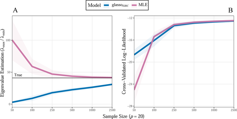
A) Eigenvalue (λ) estimation. The maximum eigenvalue was divided by the smallest eigenvalue. The true value is denoted with the grey line. A “well-conditioned” estimate will have a small disparity between these values. B) Predictive accuracy measured with k-fold cross-validation. This measure is based on the likelihood, with larger values indicating superior predictive accuracy (i.e., maximizing the likelihood). The ribbons denote one standard deviation.
Cross-Validation.
We assessed predictive accuracy with k-fold (K = 5) cross-validation, where the estimate of Θ was used to compute the cross-validated log-likelihood. We used the same simulation procedure as above, including the true covariance matrix and sample sizes. The data were first partitioned into 5 non-overlapping subsets Xk, k ∈ {1, …, 5}. We denote the training data as X−k and the test data as Xk. The prediction error, herein referred to as the cross-validated log-likelihood LCV, was then obtained as
| (7) |
Here is the inverse covariance matrix estimated from the training data , and is the covariance matrix obtained from the test data . For one simulation trial, as indicated by the summation, was averaged across the k-folds. The final estimate, for each simulation condition, was then averaged across 500 simulation trials which accounted for variability in the partitions. Further details about this procedure can be found in Gao et al. (2009) and Bien and Tibshirani (2011).
These results are presented in Figure 1 (panel B). Of course, since this measure is based on the log-likelihood, larger values indicate a more accurate estimate (i.e., maximizing the likelihood). The y-axis denotes the estimate for , whereas the x-axis includes the sample sizes n. These results reveal a similar patter as for eigenvalue estimation, in that the largest p/n value showed a clear advantage for glassoEBIC. That is, when there were 20 variables (p) and only 50 observations (n). However, as the sample size increased, this advantage dissipated quickly. For example, even with n = 100, ℒCV (the mean) indicated that the MLE was already more accurate than glassoEBIC. The estimates were ultimately very similar, with increasing sample sizes, thus indicating that ℓ1-regularization converges to the MLE in these situations (Kuismin & Sillanpää, 2016).
Summary.
These two motivating examples suggest that glassoEBIC is advantageous in situations approaching high-dimensions (p → n). However, when the sample size became similar to those commonly used to estimate psychological networks, the maximum likelihood estimate (Equation: 6) often out-performed glassoEBIC. In particular, even without selecting variables (i.e., the MLE is fully saturated), the data was not overfit according to the cross-validated log-likelihood. Although these results suggest that certain benefits of ℓ1-regularization–improved eigenvalue estimation and predictive performance–may not be realized in the most common psychological settings, these examples did not consider the additional benefit of identifying zero-valued partial correlations. In the next section, we propose two alternative methods for identifying zero-valued edges, each of which does not make use of regularization (i.e., non-regularized). The first approach, based on multiple regression, builds upon the work of Meinshausen and Bühlmann (2006), where a brief example showed that non-regularized regression was comparable to ℓ1-regularization for estimating network models in low-dimensional settings. The second approach uses a non-parametric bootstrap strategy to estimate the precision matrix directly. Both of these methods, and specifically the decision rules for identifying non-zero effects, are novel contributions to the psychological network literature.
Network Models
Thus far, we have focused exclusively on network models in the context of precision matrix estimation. While the covariances within correspond to conditional relationships between variables in a network model, we now introduce terminology that is specific to network models. Depending on the field, undirected graphical models can refer to Gaussian graphical models, covariance selection models, or random Markov fields. Here we adopted network model, because it is common in the psychological literature (Epskamp & Fried, 2016). Let X represent a p-dimensional random variable
| (8) |
where, without loss of generality, we assume all variables have been standardized to have mean zero and variance one
| (9) |
where Ip denotes the (p, p) dimensional unit matrix. Following common notation, the graph (i.e., network) is then denoted by = (V, E) and consists of nodes V = {1, …, p}, as well as the edge set (conditional relationships) E. The maximum number of edges is then , which corresponds to the unique elements in the off-diagonal of . When two variables share a conditional relation, as indicated by a non-zero partial correlation (i.e., edge), it is included in E. The aim of the present paper is to, for the first time, compare the commonly used glassoEBIC method (Epskamp, 2016; Epskamp & Fried, 2016) to a set of non-regularized methods that use multiple regression and a non-parametric bootstrap scheme for estimating these conditional relationships.
Neighborhood Selection
We first describe a regression based approach for estimating psychological networks. The regression strategy for estimating conditional relationships is called neighborhood selection (Li & Zhang, 2017; Meinshausen & Bühlmann, 2006; Yang, Etesami, & Kiyavash, 2015), which takes advantage of the correspondence between and node-wise multiple regression. The technique can be described with traditional regression notation, in which p multiple regression models are fitted. First let each node Vp be defined as y that is the scores of the n subjects on the jth variable/node.. Each node is regressed on the remaining p − 1 variables, which estimates the “neighborhood” for each variable
| (10) |
where ε is an n-dimensional vector, with the mean as a vector of zeroes, and the covariance matrix as σ2In. Here X is a n × (p − 1) design matrix and β is (p − 1) × 1 vector. The intercept is excluded, due to standardizing the data, so contains p − 1 regression coefficients. To be clear, denotes the vector of coefficients for the jth regression model, where the individual elements are defined as . The residuals are assumed to follow , where is the residual variance for the jth node.
These estimated regression coefficients and error variances have a direct correspondence to , for example,
| (11) |
where denotes the covariance corresponding to ith row and jth column of . The diagonal of is then denoted . This relationship is exact, with proofs in Stephens (1998) and further information provided in Kwan (2014). From each regression model, the coefficients and zero-entries are placed into a p × p matrix; that is, the soon to be partial correlation matrix in which each row corresponds to the neighborhood of conditional relationships for . Because the off-diagonal elements, corresponding to the lower and upper triangles of the matrix will be different when using the regression approach (i.e., proportional to ), the partial correlations are commonly computed as
| (12) |
In low-dimensional settings (p < n), these estimates are typically equivalent to standardizing the elements of and reversing the sign (Equation: 2; Krämer, Schäfer, & Boulesteix, 2009). For a pair of nodes, there are two approaches to determine whether an edge is non-zero: The “and-rule” requires both βij and βji to be determined as non-zero. On the other hand, the “or-rule” requires only one of these to be non-zero. Here, for the methods described below, when only one coefficient is non-zero we assume this is the value for the partial correlation. Thus, from the p regression models, a p × p matrix is obtained that corresponds to the underlying structure of . Of course, to estimate the neighborhood of conditional relationships, a decision rule is required for determining non-zero estimates. We propose two decision rules in the following section, each of which is novel in the context of estimating networks models.
Forward Search
We adopt two decision rules for determining non-zero coefficients, each of which uses a forward search strategy through the model space (Forward search strategy). Assume, without loss of generality, both the outcome Vp = y and design matrix X (defined in Equation: 10) have been standardized to have mean zero and variance one. This notation departs from above, slightly, but is used to be consistent with customary notation for describing information criterion. By using a forward search strategy, with the model Mi ⊂ , the objective is to select one predictor variable from V−p (denoting the pth node has been removed) that minimizes some criterion. This automated procedure is repeated until no variable within V−p can further reduce the criterion compared to the previous step. We then assume the selected variables are non-zero, thus providing the neighborhood for the predicted variable Vp.
Algorithm Forward search strategy
-
1:
Start with an empty model for each node Vp = y.
-
2:
Search to find one node ∈ V−p that minimizes AIC (Equation: 13).2
-
3:
Place the selected node into the design matrix X until the search is complete.
-
4:
Repeat steps 2 and 3 until AIC cannot be futher minimized.
-
5:
Set the regression coefficients for the excluded nodes to zero .
-
6:
Place the non-zero and zero coefficients into the jth row of a p × p matrix P (i ≠ j).
-
7:
After the last node-wise regression compute the partial correlation matrix (; Equation: 12).
Akaike Information Criterion.
The first decision rule for determining E uses the Akaike Information Criterion (AIC). There are at least two justifications for AIC based model selection, or in this case neighborhood selection: 1) expected out-of-sample prediction, since AIC and leave-one-out cross validation are asymptotically equivalent (Zhang & Yang, 2015); and 2) minimizing Kullback–Leibler (KL) divergence from the target and approximating data generating model (Burnham & Anderson, 2004). Due to strong theoretical justification, based on information theory (McElreath, 2016), we frame the neighborhood selection problem in terms of minimizing KL-divergence (Kullback & Leibler, 1951). In other words, at each forward step, we seek one variable that minimizes the following equation
| (13) |
where is the log predictive density and k is the number of parameters (i.e., the number of non-zero edges) in Mi. For the rest of the forward search, each selected variable is included in X. The decision rule for β ≠ 0 is inclusion in the final model when AIC cannot be further reduced.
Bayesian Information Criterion.
The Bayesian information criterion also has two justifications: (1) expected out-of-sample prediction, since minimizing BIC is equivalent to leave-v-out cross-validation, where v = n[1 − 1/(log(n) − 1)] (Shao, 1997); and (2) minimizing BIC approximates selecting the most probable model, assuming the true model is in the candidate set (Raferty, 1995). Due to the connection to Bayesian methods, which similarly provides strong theoretical justification (Wagenmakers, 2007), we frame neighborhood selection in terms of posterior model probabilities. The posterior probability of Mi ⊂ follows
| (14) |
where P (y|Mi, θi) is the likelihood, θi is the vector of parameters for the ith model, and P (θi) the prior distributions for θi. With a forward search strategy (Algorithm: Forward search strategy), we select one variable from V−p that maximizes P (Mi|y). Said another way, at each forward step, we select a variable that minimizes
| (15) |
The decision rule for β ≠ 0 is inclusion in the final model when BIC cannot be further reduced.
Non-Parametric Bootstrap
We now describe an approach to estimate directly. This is the same method as in the Motivating Examples, but with the addition of a decision rule to set covariances to zero. We also provide further details about the chosen inversion method that uses the singular value decomposition (Schäfer & Strimmer, 2005a). The maximum likelihood based covariance matrix, obtained with Equation 6, can be decomposed as
| (16) |
where U and V are p × p matrices containing the eigenvectors computed from Σ, and D is diagonal matrix of p eigenvalues. It is then straightforward to invert the covariance matrix, with the generalized inverse procedure (Schäfer & Strimmer, 2005a), that follows
| (17) |
Of course, this only provides a point estimate for each element of Θ which then requires a decision rule for determining E. We propose using a non-parametric bootstrapping procedure, with replacement, where percentile based confidence intervals (i.e., α levels) are used to determine the conditional relationships (Efron & Tibshirani, 1994). Although thresholding with p-values is possible with the R package qgraph, the present procedure readily provides a measure of uncertainty that allows for extending inference beyond determining significant effects–e.g., comparing edges within or between networks. For each bootstrap sample, b ∈ {1, …, B}, the estimated graph is obtained with the following steps:
Randomly sample, with replacement, n rows from the data matrix of dimensions n × p.
Compute the maximum likelihood estimate for Σb (Equation: 6).
Decompose of Σb (Equation: 16).
Compute the generalized inverse of the covariance matrix (Equation: 17), resulting in the precision matrix .
Convert to corresponding partial correlation matrix Pb.
With the B bootstrap samples in hand, it is then possible to compute the mean of a given partial correlation as whereas determining E requires obtaining a confidence interval. We use the percentile based method, with the intention of categorizing each partial correlation as 0 or 1. That is, the adjacency matrix A is constructed as
| (18) |
where denotes the lower percentile of the bootstrap samples. In words, when 0 is within the bounds of the 100(1 - α) interval, it is not included in E. To our knowledge, there is no theoretical justification for using this approach to automatically perform variable selection (Lysen, 2009), but it would still be possible to control error rates in practice (Drton & Perlman, 2004). Acknowledging this limitation, we include this method as a point of reference and without a correction for multiple comparisons.
Simulation Studies
In the psychological network literature, opposing network estimation methods are not commonly compared (to our knowledge), rather a single technique (i.e., ℓ1-regularization) has been examined across many simulation conditions (Epskamp, 2016; Van Borkulo et al., 2014). The exception is Epskamp, Kruis, and Marsman (2017), where a non-regularized method and a low-rank approximation, was used to estimate fully connected Ising models (i.e., the edge set was not determined). We thus followed common simulation procedures in psychology (Epskamp, 2016; Epskamp & Fried, 2016), but also compared performance between competing methods. We performed two different simulations, each of which was meant to answer distinct questions about the performance of the methods under consideration. The first used empirical partial correlations estimated from an actual data set (Section: Empirical Partial Correlations), whereas the second used simulated data to specifically evaluate performance across varying degrees of sparsity (i.e., the proportion of total edges that are connected; Section: Synthetic Partial Correlations).
Performance Measures
We considered two measures to capture the accuracy of the estimated partial correlations. The first was the correlation between the true partial correlations and the estimated partial correlations. In addition, we computed the sum of squared errors for each trial and then mean squared error was obtained by averaging across simualtion trials (Schäfer & Strimmer, 2005a). Lower values indicated less discrepancy from the true values such that the best method was closest to zero. For edge set identification, we considered three measures of binary classification performance that are computed from the number of true and false positives (TP and FP) and true and false negatives (TN and FN). The first two measures are sensitivity (SN), the true positive rate, and specificity (SPC) which is the true negative rate. Sensitivity is analogous to “power”, where a score of 0.50 would indicate only half of the true edges were detected. Importantly, SPC corresponds to 1 - the false positive rate, so we will often refer to both when describing the results. (1 − SPC = the false positive rate)
| (19) |
We also wanted to include a measure that considers all aspects of binary classification. To our knowledge, Matthews correlation coefficient (MCC) is the only measure that meets this criteria. The MCC is defined as
| (20) |
MCC can range between −1 and 1 (Powers, 2011). Its value is equivalent to the phi coefficient that assesses the association between two binary variables, but for the special case of binary classification accuracy. These measures were averaged across simulation trials.
Computation and Software
All computations were done in R version 3.4.2 (R Core Team, 2016). We performed 1,000 simulation trials for each of the conditions, and recorded the elapsed time to fit each estimation procedure. The glasso method was fitted with the R package qgraph version 1.5 (Epskamp, Cramer, Waldorp, Schmittmann, & Borsboom, 2012), where we used the default settings. The non-regularized methods were fitted with a custom function that used the package bestglm for the forward search (Mcleod & Xu, 2017), whereas the non-parametric bootstrap did not make use of any R packages. All of the non-regularized methods have been implemented in the R package GGMnonreg. The simulation code is publicly available online (Code: Open Science Framework).
Empirical Partial Correlations
For this simulation study, we estimated the sample partial correlation matrix from a well-known area of research in clinical networks; that is, post-traumatic stress disorder symptoms (PTSD). These data are on a 5 value ordinal scale, including 221 observations (n) and 20 variables (p). It should be noted that we estimated Pearson correlations (as opposed to polychoric correlations), which are known to be attenuated in the case of ordinal data. This decision was made for two reasons: (1) it is common to assume normality for ordinal data (Rhemtulla, Brosseau-Liard, & Savalei, 2012); (2) when preparing the simulations, we noted that the glasso method struggles with larger values, so computing Pearson correlations was more favorable to the current default approach in psychology. We then followed the approach described in Schäfer and Strimmer (2005b) and Krämer et al. (2009), where new graphical structures were generated at each simulation trial. The network structure (connections between variables) was therefore random. So while the partial correlations values were assumed to be representative of a specific clinical application (Figure: 2), our results are not conditional on a specific network structure. These steps were followed for each simulation trial:
Randomly sample one p × p matrix p ∈ {10, …, 20} from the partial correlation matrix estimated from the PTSD data set, and then set absolute values less than 0.05 to zero (Epskamp, 2016).
Convert the sampled partial correlation matrix to a correlations matrix, and assume this is the covariance structure for the p variables.
Generate data (continuous and 5-level ordinal) with samples of size n ∈ {100, 250, 500, 1000, and 2, 500}.
- Estimate the networks with the following three methods:
- glassoEBIC (γ = 0.5)
- Node-wise regression models were fitted with the previously described decision rules (i.e., AIC and BIC). For these models, we included both the “and-rule” and “or-rule” that was described above (Section: Neighborhood Selection). For the “or-rule”, we assumed the partial correlation was equal to the one non-zero coefficient. We report the “or-rule” in the body of the text, while the “and-rule” is presented in the Appendix. We also plotted the “or-rule” and “and-rule” together, which allows for comparing their performance (also provided in the Appendix).
- Non-parametric bootstrap to directly estimate the precision matrix. The confidence level was set to 99 % (i.e., α = 0.01) and 1,000 bootstrap samples were generated.
Compute performance measures.
For the ordinal data, generated with the package bootnet version 1.0.1 (Epskamp, Borsboom, & Fried, 2018), we assumed normality for the non-regularized regression approaches. For glassoEBIC, we followed the default settings and estimated polychoric correlations. This served as a valuable comparison, because it allowed for characterizing one important limitation of the regression based approaches that cannot estimate polychoric correlations. The non-parametric boostrap approach also estimated Pearson correlations, although it would be possible to estimate polychoric correlations.
Figure 2.
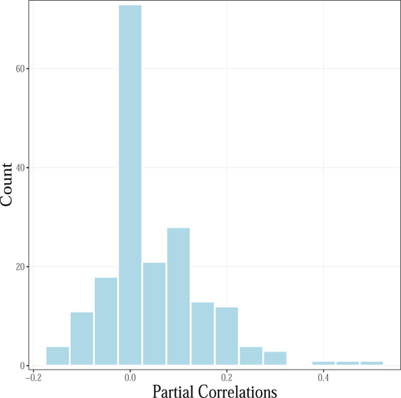
The distribution of empirically estimated partial correlations. These were sampled from to generate the partial correlation matrices for the first simulation study (Section: Empirical Partial Correlations).
Results.
Before discussing the results, we reiterate the primary goal of this work. Our objective is not to suggest non-regularized methods are “significantly” better than glassoEBIC. Rather, while methods optimized for high-dimensional settings were readily adopted as the default approach, it remains unclear whether they have advantages compared to traditional statistical methods. For example, the properties of non-regularized model selection with BIC are well known in the social-behavioral sciences (p < n), but the extension to regularized estimation with EBIC was primarily made to address situations that are uncommon in the network literature (i.e., n < p or p → n).
We first discuss the timing results that are displayed in Figure 3. The introduced methods are computationally intensive, which could limit their use in practical applications. Indeed, for most of the simulation conditions glassoEBIC was the fastest approach. However, the differences between glassoEBIC and regression were often small. Each of these methods typically took less than one second, with the exception being glassoEBIC for ordinal data (p = 20). Here the default in the qgraph package is to estimate polychoric correlations, which is apparently computationally intensive, whereas normality was assumed for the non-regularized methods (Rhemtulla et al., 2012). On the other hand, the non-parametric bootstrap strategy was the slowest method, with the elapsed time being influenced by the sample size. Of course, this is the only method to provide a measure of uncertainty for the edges, and it was recently shown that bootstrapping glassoEBIC (B = 2,000) took almost 20 minutes (Williams, 2018). This should be noted when interpreting these results.
Figure 3.

Elapsed time for estimating each model. The glasso method estimated polychoric correlations for the ordinal data, whereas the non-regularized methods estimated Pearson correlations.
We now discuss the results for accurate estimation of the partial correlations, as measured by correlations and mean squared error (true vs. estimated). For the body of the text, the results have been simplified to improve clarity and highlight specific findings. Here we primarily focus on p = 20, the number of variables in the PTSD data set, with the remaining results provided in the Appendix. For the continuous data (Figure: 4; the left panel), the regression methods (AIC and BIC) had similar performance compared to glassoEBIC for the largest samples sizes. For MSE in particular, glassoEBIC had superior performance for the smaller sample sizes. This was also the case for the ordinal data. Note that, for samples larger than 250, the correlations were similar between methods. The exception was for the smallest sample size (n = 100), where glassoEBIC had the lowest correlations. This was likely due to estimating empty networks for some of the simulation trials. Of note, while the differences were not large, AIC based model selection consistently had the highest correlation and lowest MSE among the non-regularized methods. In fact, these results make it clear that directly estimating does not necessarily result in more accurate estimates. The regularized method did offer some advantages, in that the MSE was often the lowest. This was especially the case for ordinal data, where polychoric correlations were estimated. However, this was not the case for the smaller networks (Figure: A1; p = 10). Here the opposite pattern emerged, in that glassoEBIC rarely had the best (referring to the average across simulation trials) performance scores.
Figure 4.
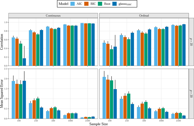
Simulation results of the larger networks (p = 20). The glasso method estimated polychoric correlations for the ordinal data, whereas the non-regularized methods estimated Pearson correlations. The error bars denote one standard deviation.
Accurate estimation is important, but an arguably more important goal is identifying the edge set. We thus spend more time describing these results, which are displayed in Figure 5. We begin with the top row, that includes the results for specificity, and then work our way down to the MCC scores. Before interpreting the results, we again note that 1 − the false positive rate is equivalent to specificity (SPC). The results immediately point towards a potential issue with glassoEBIC, in that SPC consistently decreased with larger sample sizes. In other words, with increasing information, the regularized method made increasingly more false positives. For continuous data, the false positive rate was around 0.10 (n = 100), whereas it was greater than 0.30 for the largest sample size (n = 2, 500). It is possible to infer the number of false positives, assuming the average sparsity was ≈ 0.45, in relation to the number of covariances . That is, for n = 2, 500, the number of false positives was roughly 190 × 0.45 × [1 − 0.67] ≈ 28. On the other hand, the boostrap method with 99 % confidence intervals had the nominal error rate for the same condition (α = 0.01), resulting in approximately 1 false positive for a given simulation trial (190 × 0.45 × [1 − 0.988] ≈ 1). Further, the regression approach using BIC showed the opposite pattern as glassoEBIC, where more information resulted in improved edge identification. That is, for each increase in n, SPC consistently improved to be 0.991 for the largest sample size (n = 2,500). As a reminder, for the same condition, SPC was less than 0.70 for glassoEBIC. A similar pattern was observed for the ordinal data, although each method showed a slight decrease in SPC compared to continuous data. However, the non-regularized methods clearly had the lowest false positive rate (n > 100), thereby indicating that the assumption of normality did not present issues for identifying the edge set.
Figure 5.
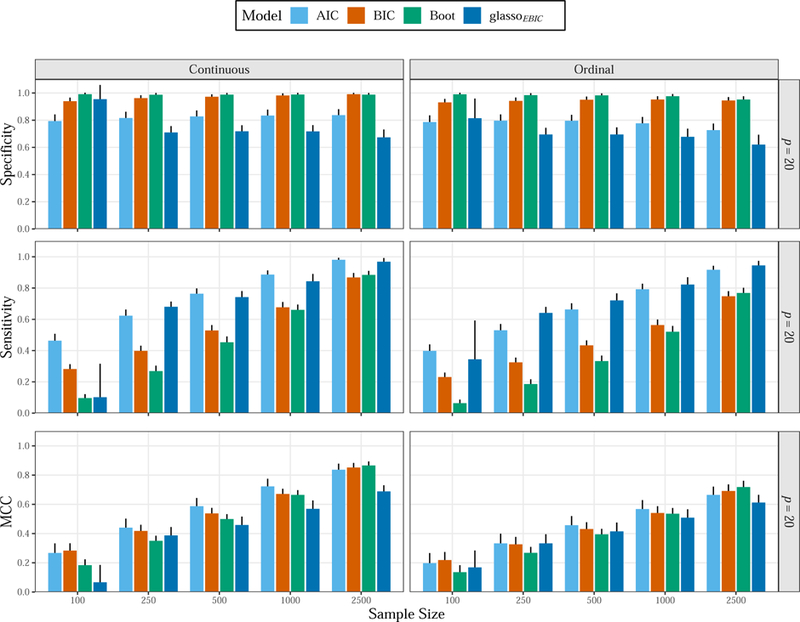
Simulation results of the larger networks (p = 20). Specificity (SPC) is the true negative rate and 1 - SPC is the false positive rate. Sensitivity is the true positive rate. This is analogous to the “power” to detect the true edges for a given network. The glasso method estimated poly-choric correlations for the ordinal data, whereas the non-regularized methods estimated Pearson correlations. The error bars denote one standard deviation.
The results for sensitivity are displayed in the middle row (Figure: 5). By definition (Equation: 19), sensitivity (SN) is the proportion of true positives that were detected. For p = 20, it is similarly possible to infer the number of detected edges as 190 × 0.55 × SN, where 0.55 is 1 - the sparsity level. Interestingly, while glassoEBIC showed the lowest specificity among the methods, SN was not always the highest for continuous data. Here regression with AIC had comparable ability to detect edges, but had higher SPC that did not diminish with more information (i.e., larger sample size). This is important in practical applications, when considering the false discovery rate (FDR)3. For n = 2500, the FDR was approximately 0.21 for glassoEBIC. That is, approximately 1 out of 5 edges detected by glassoEBIC was a false discovery. On the other hand, it was less than 1 % for BIC based model selection with ordinary least squares. Of note, the non-regularized methods did have lower SN for ordinal than continuous data, indicating one limitation of assuming normality.
We end this section discussing Matthews correlation coefficient (Figure: 5; bottom row). As previously motioned, the MCC incorporates all aspects of binary classification, and is a correlation between binary variables. Here glassoEBIC had the highest score once (i.e.,ordinal data and n = 250), although the difference from AIC was very small. When considering p = 10, resulting in 20 conditions in total, regularized estimation only had the best score that one time. On the other hand, the regression approach with AIC consistently had the highest MCC scores. The exception was for the largest sample size (n = 2, 500), although the score was still higher than glassoEBIC.
Synthetic Partial Correlations
For this simulation study, we investigated method performance in relation to network sparsity. This serves two purposes. First, accurate model selection for ℓ1-regularization depends on strong assumptions, most notably of which is that few very effects are non-zero. This can refer to coordinate (in regression) or row sparsity (in the case of the glasso; Janková & van de Geer, 2017), but for our purposes it suffices to state common simulation scenarios in the statistics literature to demonstrate model selection consistency. It is common to assume less than 5 % of the effects are non-zero (Waldorp, Marsman, & Maris, 2018), or in some instances not even 1 % (Bühlmann & Van De Geer, 2011). Further, when the sparsity assumptions is violated, the necessary (for model selection consistency) irrepresentable condition is almost never satisfied (P. Zhao & Yu, 2006). This condition is difficult to examine in practice, but essentially states that the relevant and irrelevant variables may not be (highly) correlated with one another. In P. Zhao and Yu (2006), with synthetic data generated from a Wishart distribution, they showed that this assumption was often met with very few non-zeroes (i.e., a sparse model), but was almost never satisfied when over half of the effects were non-zero which appears to be common in psychological applications. Second, this allowed for examining the decision rule based on α levels, that did not include a correction for multiple comparisons.
We assumed one sample size (n = 500), two values for p ∈ {10 and 20}, and 5 sparsity levels η ∈ {90%, 80%, 70 %, 60 %, and 50%}. Two representative graphical structures can be found in the Appendix (Figure: A14). The magnitude of the partial correlations also varied by adjusting the degrees of freedom of the G-Wishart distribution, corresponding to 90 % of the partial correlations within ± 0.40 for the former and 90 % within ± 0.25. That is, we adjusted the degrees of freedom such that there was a 2 × 5 × 2 simulation design: two values for the number of variables × five sparsity levels × two different partial correlation ranges. As pointed out by a reviewer, when the network becomes more connected, the partial correlations must be smaller to ensure the matrix is positive definite. We accounted for this by determining which degrees of freedom, for given sparsity level and network size, resulted in the previously stated ranges. As such, the only thing that varied in this simulation study was sparsity and the partial correlation sizes. These distributions were approximately normal, such that smaller values were sampled more often than larger values. Of note, the G-Wishart distribution is a generalization of the Wishart distribution, with some off-diagonal elements in the precision matrix constrained to be zero. The network structure was again random, and all generating matrices were positive definite. For each trial, of which there were 1,000, the simulation procedure followed:
Generate data n = 500 from a p dimensional G-Wishart distributed precision matrix Θ ∼ WG(df, Ip), where Ip is a p dimensional identity matrix (Mohammadi & Wit, 2015b).
Fit the same models as in the previous simulation study (Section: Empirical Partial Correlations).
Compute performance measures.
Results.
The results are displayed in Figure 6. We focus on the false positive rate for both network sizes (p = 10 and 20), with the remainder of the results provided in the Appendix. As a reminder, the sample size has been fixed (n = 500) and the primary objective is to evaluate the influence of sparsity and partial correlation size on edge set identification. There are striking differences between the non-regularized methods and glassoEBIC. The boostrap method in particular, described above (Section: Non-Parametric Bootstrap), provides an interesting contrast because there is an expected error rate (α = 0.01). Here, irrespective of sparsity and partial correlation size, the error rate was consistently at the nominal level. In other words, α can be used to directly control specificity which stands in contrast to glassoEBIC, where neither lambda (Equation: 4) or gamma (Equation: 5) have a direct correspondence to edge identification. Further, the accuracy of glassoEBIC was influenced by the sparsity level and partial correlation size. For example, with the larger partial correlations (±0.40), the error rate was below 0.10 for the sparsest network, but consistently increased to be over 0.40 when sparsity was 50 %. The error rate was lower for the smaller partial correlations (±0.25), but also increased as the networks became more dense. Of note, the regression approach with BIC was also affected by the sparsity level in that the error rate also increased with denser network. However, not only was this less pronounced than glassoEBIC, the “and-rule” did not show this increase in false positives (Figure: A9).
Figure 6.

Simulation results (n = 500). The ± denotes that 90 % of the partial correlations were in that range. Sparsity is the probability an edge was zero for a given network. Sparsity decreases when moving from the left to right. The error bars denote one standard deviation.
Discussion
In this paper, we compared the most popular estimation method for estimating psychological networks, the graphical lasso, with a number of non-regularized methods that can be used to estimate networks in low-dimensional settings (i.e., when p << n). We found that the non-regularized methods typically out-performed the graphical lasso. Most notably, whereas non-regularized methods showed better performance with increasing n, for glasso increasing n simultaneously increases sensitivity to detect conditional relationships and steadily inflates the false positive rate (1 - specificity). This lack of (model selection) consistency is particularly problematic in the context of psychological network estimation where researchers typically aim to estimate a network among a fixed set of variables (p) with the largest sample size (n) possible. Second, as the true connectivity of networks became more dense, the false positive rate substantially increased for glassoEBIC, whereas this increase was far less pronounced for the non-regularized methods based on multiple regression and there was no increase for the non-parametric bootstrap strategy. Third, the performance of glassoEBIC varied substantially as a function of the range of partial correlations (edge strengths) in the generating model, whereas non-regularized estimates were more stable. Although these findings build a strong case for using non-regularized methods in practice, we would prefer that applied researchers justify their method choice. The present results, as well as the following exposition, can provide a foundation for building this rationale.
The glasso method offers two potential advantages over maximum likelihood estimation: (1) regularization–shrinkage–that can either improve the estimate of the precision matrix, or ensure the matrix can be computed altogether (n < p); and (2) improved predictive accuracy. We demonstrated that these benefits may not be appreciable when estimating psychological networks in low-dimensional settings (p ≪ n). First, the improved properties of the precision matrix (i.e., eigenvalue estimation), which allows for more accurate estimation, steadily diminished with increasing sample sizes to ultimately be comparable to maximum likelihood. Second, the improved predictive accuracy of glassoEBIC, as measured by the cross-validated log-likelihood, similarly diminished with increasing samples sizes.
For estimating networks, we introduced two non-regularized estimation methods that rely on multiple regression with forward selection and a non-parametric bootstrap strategy. To our knowledge, in the context of network estimation, these methods each included a novel decision rule for determining conditional relationships. With extensive numerical experiments, we demonstrated that the non-regularized approaches consistently recovered the true network with increasing sample sizes. In contrast, the performance of glassoEBIC, with respect to specificity, decreased with larger samples sizes. This suggests that glassoEBIC does not provide consistent model selection for common applications of network modeling in psychology. Further, we examined how the false positive rate is influenced by sparsity which showed that glassoEBIC was especially sensitive to the overall connectivity of the network (Epskamp et al., 2017). Of course, while the exact definition of sparsity is a subjective one, many network models show over 50 % connectivity and ℓ1-based approaches assume only a small proportion will be non-zero for accurate edge set identification (Figure: 6; P. Zhao & Yu, 2006). We would argue that it is unreasonable to suggest this level of connectivity exemplifies sparsity, which then influences the accuracy with which the network is estimated. For constructs such as personality traits and psychiatric symptoms, one could argue that the statistical assumption of sparsity is questionable. The present results suggest that the non-regularized methods are less sensitive to this assumption, and therefore offer advantages in this respect compared to glassoEBIC.
Non-regularized Methods in Practice
The primary goal of this work was to compare non-regularized methods to glassoEBIC. It was revealed that partial correlation networks can readily be estimated with tools already well-established to the social-behavioral sciences. Building on this information, but applied to networks, it makes sense that AIC had a higher false positive rate than BIC and that confidence intervals can readily be used to control specificity (1 - α). In other words, although network models are novel to psychology, the information provided in countless methodological papers applies to estimating psychological networks. For example, Casella et al. (2009) and Bollen, Harden, Ray, and Zavisca (2014) that use BIC for model selection and Burnham and Anderson (2004) that makes clear the distinction between AIC and BIC. The importance of this cannot be understated, in that it allows for applied network researchers to use and review methods that they are more familiar with. For example, to our knowledge, it has not once been stated why BIC was extended in the first place. According to Chen and Chen (2008), who introduced EBIC, “…yet our consistency result has extended our understanding of the original BIC for the small-n–large-P problem”, where it is clear BIC was extended to address a problem uncommon to psychology. Indeed, in that work, the applied example with real data included 233 observations (n) and 1414 variables (p).
We found that, for the regression based approaches, not much was gained from applying the more conservative “and-rule.” Here both specificity and sensitivity were similar for both decision rules. The one notable difference between decision rules was for sparsity, where the “and-rule” provided consistent edge identification across sparsity levels (Figure: A8). Interestingly, it was also revealed that direct estimation does not necessarily lead to more accurate estimates than using multiple regression. This could have been due to detecting fewer edges, thus error would naturally increase. In support of this notion, AIC was best among the non-regularized methods for the correlations and MSE. However, as shown throughout the simulation results, the direct method based on confidence intervals allows for calibrating to a desired level of specificity. These methods have been implemented in the R package GGMnonreg.
Comparison to Previous Simulations
Although glasso has emerged as the default approach for network estimation in psychology, and is a very popular method outside of psychology (Kuismin & Sillanpää, 2017), there have been many alternative methods that have shown superior performance. It should first be noted that, while the original glasso paper is highly cited (Friedman et al., 2008), no comparisons were made to alternative methods with respect to edge identification. In fact, when measuring cross-validation error, it was demonstrated that a non-regularized method was superior to glasso when p < n (Bien & Tibshirani, 2011; Friedman et al., 2008). According to Friedman et al. (2008), “…cross-validation curves indicate that the unregularized model is the best, [which is] not surprising given the large number of observations and relatively small number of parameters” (p. 9). Their conclusion is consistent with our results, and we further demonstrated reduced prediction error with increasing samples sizes for the maximum likelihood estimate. Further, the paper that introduced the method of using EBIC to select the tuning parameter (λ) similarly did not make comparisons to other network estimation methods (Foygel & Drton, 2010). Rather, the focus was on alternative γ values in comparison to using cross-validations for selecting λ. This parallels the psychological network literature, where to our knowledge the glassoEBIC method has never been directly compared to alternative estimation methods.
However, since the introduction of the glasso method in Friedman et al. (2008), there have been numerous papers that have compared novel methods to glassoEBIC. Most recently, for example, Williams et al. (2018) introduced a Bayesian approach based on predictive loss and used the horseshoe prior distribution for regularization purposes (Carvalho, Polson, & Scott, 2010; Piironen & Vehtari, 2017). They showed that glassoEBIC rarely had the best performance among three methods for accurately detecting edges. Similarly, Leppä-aho, Pensar, Roos, and Corander (2017) introduced an approximate Bayesian method, using a marginal pseudo-likelihood approach, that showed glassoEBIC was not always consistent with respect to Hamming distance (Norouzi, Fleet, Salakhutdinov, & Blei, 2012), whereas the lasso regression approach was consistent. Moreover, Mohammadi and Wit (2015a) compared their proposed Bayesian method, based on posterior model probabilities, to glassoEBIC. They also included the StARS and RIC methods for tuning parameter selection. In addition to the Bayesian method showing superior performance compared to glassoEBIC, both StARS and RIC also showed clear advantages compared glassoEBIC. This is particularly interesting for psychology, because the simulation conditions were primarily in low-dimensional settings (p < n). There are several additional methods that have been shown to outperform glassoEBIC, but a thorough discussion is beyond the scope of this paper. We refer interested readers to Kuismin and Sillanpää (2017), where they review numerous methods as well as the benefits and limitations of each.
Limitations
There are several important limitations of the present research. First, although we argued that inferences from regularized methods are not straight forward, the non-regularized methods did not explicitly address these limitations. As such, a limitation of the present work is that we have only provided one method for making inference about individual partial correlations–the bootstrap approach–which would also require corrections for multiple comparisons in practice. Of course, ℓ1-regularization only provides a point estimate and would also require corrections if attempting to make inference (assuming one could obtain valid standard errors). However, there are several reasons to prefer the non-regularized approaches. The limitations of automated model selection are known for traditional methods (Harrell, 2001), and this readily allows for the research community to critique inferences that are extended beyond the exploratory nature of this approach. Note that we only used forward selection that is not without problems4. For example, it could be that sequentially adding predictors will not converge on the true model. However, our results revealed that performance can be very good compared to the current default estimation method in psychology. Furthermore, methods and corresponding inferences that are unfamiliar to psychologists are much more difficult to evaluate and critique.5 Additionally, while inference is possible from lasso estimates, their asymptotic properties (e.g. α) are often evaluated in high-dimensional settings (Bühlmann, 2012). However, there are methods that allow for valid inference in low-dimensional settings when forward selection has been used (Benjamini & Gavrilov, 2009; Blanchet, Legendre, & Borcard, 2008).
Second, our primary simulation results were obtained from empirically derived partial correlations. This could be problematic, because it is possible that performance would change with different partial correlations. Indeed, our simulation results showed that different partial correlation strengths affected the relative performance of the estimators. Third, our decision to not assume one network structure with fixed partial correlations values may be viewed as a limitation. However, in our experience, performance can differ substantially based on the assumed data generating matrix. As such, when a simulation study examines results under a single fixed population, the results are then conditional on that population, which in our view limits generalizability. Therefore, our simulation approach provided a measure of robustness to uncertainty in knowing the truth, such as network structure and partial correlation magnitude, although the latter were restricted to plausible ranges. Fourth, it should be noted that we did not fully characterize the performance of the non-regularized methods. For example, we did not consider a variety of graphical structures, which is commonly done when characterizing the performance of a novel method compared to existing methods. The generating matrices could have presented challenges for ℓ1-regularization, as revealed in the section Synthetic Partial Correlations. We investigated several structures (e.g., AR-1), and found that the decrease in specificity as n increased was not specific to these particular generating networks. We further found that glassoEBIC can have excellent performance as n increases, but this required strong assumptions regarding sparsity (η ≈ 0.95), which parallels the findings in Figure 6. The decision to use this particular simulation procedure, in particular the empirically derived partial correlations, was made because we wanted to make our results comparable to the recent psychological literature on network models: (1) Epskamp (2016) used empirical partial correlation and set absolute values less than 0.05 to zero; and (2) Epskamp and Fried (2016) also used these post-traumatic stress data for simulation purposes and an applied example.
Fifth, we also did not consider ℓ2-regularization, for example ridge regression that is commonly used in the context of prediction (de Vlaming & Groenen, 2015; Hoerl & Kennard, 1970). This differs from lasso regression, in that variable selection (i.e., estimation of exact zeroes) is not achieved by minimizing the residual sums of squares with respect to the penalty term. It is also possible to obtain a ridge-type estimator of the covariance matrix, for example with the approach described in Van Wieringen and Peeters (2016) and Kuismin et al. (2017). These approaches require a decision rule for setting values to zero. A common approach for computing p-values, with ridge-type estimators, relies on constructing a null sampling distribution which also makes strong assumptions about sparsity and have primarily been characterized in high-dimensional settings (Schäfer & Strimmer, 2005a). Further, to our knowledge, only ℓ1-regularization has been used to estimate psychological networks. For these reasons we did not consider ℓ2-regularization, although it should be noted that ridge approaches may offer some advantages for psychology in particular (as point out by an anonymous reviewer). For example, assuming small effects are common in psychology, ℓ2-based methods could preserve these effects by proportionally shrinking all of the edges and not pushing them to zero.
Sixth, our primary objective was to characterize method performance across a variety of simulation conditions. We did not extensively discuss the practical implications of a 40 % false positive rate (Figure: 5), although we did relate this to the false discovery rate (FDR) in the results section. The magnitude of the false positives is important to consider; that is, whether they were small or large would have differing effects on network interpretation. Assuming the false positives were small in size, they may not be detrimental for interpreting which relations are the strongest, but would certainly affect inferences regarding global characteristics including overall connectivity and neighborhood size. For the boostrap method, the false positives will necessarily be large, at least 1.96 × the standard error away from zero (assuming a 95 % confidence interval). However, in our view, this is advantageous because researchers can readily perform null hypothesis significance tests that require nominal α levels to achieve desired error rates. In other words, to make customary inferences about the population, sampling variability is a necessary component.
Lastly, note that there are alternative methods for estimating networks and this limits the generalizability of our findings (Kuismin & Sillanpää, 2017). However, our focus was explicitly on the most common estimation method in the social-behavioral sciences. We refer interested readers to Fan, Liao, and Liu (2016) and Kuismin and Sillanpää (2017) where alternative methods are reviewed. These reviews do not include Bayesian methods, but these can be found in Mohammadi and Wit (2015a) and Williams and Mulder (2019).
Future Directions
The present paper suggests that more quantitative work is needed on the topic of network estimation. First, these non-regularized regression approaches should be compared to alternative methods for network estimation (Kuismin & Sillanpää, 2017). Second, for glasso, alternative tuning parameter selection methods (Section: Precision Matrix Estimation) can be investigated. These topics should be examined in research settings common to psychology (p < n). Importantly, the necessary components for estimating a network, outside of ℓ1-regularization, include parameter estimation and a decision rule for including edges in a network. In fact, even for the Bayesian version of the lasso, a decision rule is needed to achieve sparsity (Khondker, Zhu, Chu, Lin, & Ibrahim, 2013; H. Wang, 2012). This does stand in contrast to fully automated procedures (e.g., that automatically set values to zero), but has the added benefit of requiring a justification for the chosen decision rule (Sections: Akaike Information Criterion and Bayesian Information Criterion). Additionally, there are many possibilities to develop or characterize existing methods specifically for psychology. For example, we only considered 5-level ordinal data and looking at different levels is an important future direction–e.g., this boostrapping scheme can be compared to glassoEBIC. Of course, there are high-dimensional settings in psychology to consider. For these fields, glassoEBIC should not be the de facto default, because several methods have been shown to have superior performance.
Conclusion
We conclude that network analysis is an important tool for understanding psychological phenomenon. Since network modeling is a burgeoning area, addressing the issues that we raised will ensure a solid methodological foundation going forward and a deeper understanding of this relatively novel statistical method.
Supplementary Material
Acknowledgments:
The authors would like to thank the three reviewers and the editor for their comments on prior versions of this manuscript. The ideas and opinions expressed herein are those of the authors alone, and endorsement by the authors’ institution, the National Institute on Aging or the National Institutes of Health is not intended and should not be inferred.
Funding: This work was supported by Grant R01AG050720 from the National Institute On Aging of the National Institutes of Health
Role of the Funders/Sponsors: None of the funders or sponsors of this research had any role in the design and conduct of the study; collection, management, analysis, and interpretation of data; preparation, review, or approval of the manuscript; or decision to submit the manuscript for publication.
Research reported in this publication was supported by three funding sources: (1) The National Academies of Sciences, Engineering, and Medicine FORD foundation pre-doctoral fellowship to DRW; (2) The National Science Foundation Graduate Research Fellowship to DRW; and (3) the National Institute On Aging of the National Institutes of Health under Award Number R01AG050720 to PR. The content is solely the responsibility of the authors and does not necessarily represent the official views of the National Academies of Sciences, Engineering, and Medicine, the National Science Foundation, or the National Institutes of Health.
Footnotes
Conflict of Interest Disclosures: Each author signed a form for disclosure of potential conflicts of interest. No authors reported any financial or other conflicts of interest in relation to the work described.
Ethical Principles: The authors affirm having followed professional ethical guidelines in preparing this work. These guidelines include obtaining informed consent from human participants, maintaining ethical treatment and respect for the rights of human or animal participants, and ensuring the privacy of participants and their data, such as ensuring that individual participants cannot be identified in reported results or from publicly available original or archival data.
TP and FP denote the number of true and false positives, whereas FN is the number of false negatives.
The same procedure applies to BIC.
The FDR is defined as . This was computed by approximating the number of false and true positives, which was done in the preceding two paragraphs, then solving the FDR equation.
We have implemented both best subset selection and backwards elimination in the accompanying R package.
To understand the inferential challenges for lasso estimates, and recently proposed methods for inference, we recommend chapter six (Statistical Inference) of Hastie et al. (2015).
References
- Armour C, Fried EI, Deserno MK, Tsai J, & Pietrzak RH (2017). A network analysis of DSM-5 posttraumatic stress disorder symptoms and correlates in U.S. military veterans. Journal of Anxiety Disorders, 45(May 2013), 49–59. doi: 10.1016/j.janxdis.2016.11.008 [DOI] [PubMed] [Google Scholar]
- Avagyan V, Alonso AM, & Nogales FJ (2017, 10). Improving the Graphical Lasso Estimation for the Precision Matrix Through Roots of the Sample Covariance Matrix. Journal of Computational and Graphical Statistics, 26(4), 865–872. doi: 10.1080/10618600.2017.1340890 [DOI] [Google Scholar]
- Benjamini Y, & Gavrilov Y (2009). A simple forward selection procedure based on false discovery rate control. Annals of Applied Statistics, 3(1), 179–198. doi: 10.1214/08-AOAS194 [DOI] [Google Scholar]
- Bien J, & Tibshirani RJ (2011, 12). Sparse estimation of a covariance matrix. Biometrika, 98(4), 807–820. doi: 10.1093/biomet/asr054 [DOI] [PMC free article] [PubMed] [Google Scholar]
- Blanchet G, Legendre P, & Borcard D (2008). Forward selection of spatial explanatory variables. Ecology, 89(9), 2623–2632. doi: 10.1890/07-0986.1 [DOI] [PubMed] [Google Scholar]
- Bollen KA, Harden JJ, Ray S, & Zavisca J (2014, 1). BIC and Alternative Bayesian Information Criteria in the Selection of Structural Equation Models. Structural Equation Modeling, 21(1), 1–19. doi: 10.1080/10705511.2014.856691 [DOI] [PMC free article] [PubMed] [Google Scholar]
- Borsboom D, & Cramer AO (2013). Network Analysis: An Integrative Approach to the Structure of Psychopathology. Annual Review of Clinical Psychology, 9(1), 91–121. doi: 10.1146/annurev-clinpsy-050212-185608 [DOI] [PubMed] [Google Scholar]
- Bühlmann P (2012). Statistical significance in high-dimensional linear models, 19(4), 1212–1242. doi: 10.3150/12-BEJSP11 [DOI] [Google Scholar]
- Bühlmann P, Kalisch M, & Meier L (2014). High-Dimensional Statistics with a View Toward Applications in Biology. Annual Review of Statistics and Its Application, 1(1), 255–278. doi: 10.1146/annurev-statistics-022513-115545 [DOI] [Google Scholar]
- Bühlmann P, & Van De Geer S (2011). Statistics for high-dimensional data: methods, theory and applications Springer Science & Business Media. [Google Scholar]
- Burnham KP, & Anderson DR (2004). Multimodel inference: Understanding AIC and BIC in model selection. Sociological Methods and Research, 33(2), 261–304. doi: 10.1177/0049124104268644 [DOI] [Google Scholar]
- Carvalho CM, Polson NG, & Scott JG (2010). The horseshoe estimator for sparse signals. Biometrika, 97(2), 465–480. doi: 10.1093/biomet/asq017 [DOI] [Google Scholar]
- Casella G, Girón FJ, Martinez ML, & Moreno E (2009). Consistency of bayesian procedures for variable selection. Annals of Statistics, 37(3), 1207–1228. doi: 10.1214/08-AOS606 [DOI] [Google Scholar]
- Chand S (2012). On tuning parameter selection of lasso-type methods - A Monte Carlo study. Proceedings of 2012 9th International Bhurban Conference on Applied Sciences and Technology, IBCAST 2012, 120–129. doi: 10.1109/IBCAST.2012.6177542 [DOI] [Google Scholar]
- Chatterjee A, & Lahiri SN (2011). Bootstrapping Lasso Estimators (Vol. 106). Taylor & Francis, Ltd. American Statistical Association. doi: 10.2307/41416396 [DOI] [Google Scholar]
- Chen J, & Chen Z (2008). Extended Bayesian information criteria for model selection with large model spaces. Biometrika, 95(3), 759–771. doi: 10.1093/biomet/asn034 [DOI] [Google Scholar]
- Cramer AO, & Borsboom D (2015). Problems Attract Problems: A Network Perspective on Mental Disorders. Emerging Trends in the Social and Behavioral Sciences(1915), 1–15. doi: 10.1002/9781118900772 [DOI] [Google Scholar]
- Dalalyan AS, Hebiri M, & Lederer J (2017). On the prediction performance of the Lasso. Bernoulli, 23(1), 552–581. doi: 10.3150/15-BEJ756 [DOI] [Google Scholar]
- Dalege J, Borsboom D, van Harreveld F, & van der Maas HLJ (2017). A Network Perspective on Political Attitudes: Testing the Connectivity Hypothesis
- Das A, Sampson A, Lainscsek C, Muller L, Lin W, Doyle J, … Sejnowski T (2017). Interpretation of the Precision Matrix and Its Application in Estimating Sparse Brain Connectivity during Sleep Spindles from Human Electrocorticography Recordings. Neural computation, 29(3), 603–642. doi: 10.1162/NECO{\_}a{\_}00936 [DOI] [PMC free article] [PubMed] [Google Scholar]
- Dempster A (1972, 3). Covariance Selection. Biometrics, 28(1), 157–175. doi: 10.2307/2528966 [DOI] [Google Scholar]
- Deserno MK, Borsboom D, Begeer S, & Geurts HM (2017). Multicausal systems ask for multicausal approaches: A network perspective on subjective well-being in individuals with autism spectrum disorder. Autism, 21(8), 960–971. doi: 10.1177/1362361316660309 [DOI] [PubMed] [Google Scholar]
- de Vlaming R, & Groenen PJF (2015, 7). The Current and Future Use of Ridge Regression for Prediction in Quantitative Genetics. BioMed Research International, 2015, 1–18. doi: 10.1155/2015/143712 [DOI] [PMC free article] [PubMed] [Google Scholar]
- Drton M, & Perlman MD (2004). Model selection for Gaussian concentration graphs. Biometrika, 91(3), 591–602. doi: 10.1093/biomet/91.3.591 [DOI] [Google Scholar]
- Efron B (2014, 7). Estimation and Accuracy After Model Selection. Journal of the American Statistical Association, 109(507), 991–1007. doi: 10.1080/01621459.2013.823775 [DOI] [PMC free article] [PubMed] [Google Scholar]
- Efron B, & Tibshirani R (1994). An introduction to the bootstrap CRC. [Google Scholar]
- Epskamp S (2016). Regularized Gaussian Psychological Networks: Brief Report on the Performance of Extended BIC Model Selection. arXiv, 1–6.
- Epskamp S, Borsboom D, & Fried EI (2018). Estimating psychological networks and their accuracy: A tutorial paper. Behavior Research Methods, 50(1), 195–212. doi: 10.3758/s13428-017-0862-1 [DOI] [PMC free article] [PubMed] [Google Scholar]
- Epskamp S, Cramer AOJ, Waldorp LJ, Schmittmann VD, & Borsboom D (2012). qgraph: Network Visualizations of Relationships in Psychometric Data. Journal of Statistical Software, 48(4). doi: 10.18637/jss.v048.i04 [DOI] [Google Scholar]
- Epskamp S, & Fried EI (2016). A Tutorial on Regularized Partial Correlation Networks. arXiv doi: 10.1103/PhysRevB.69.161303 [DOI] [PubMed] [Google Scholar]
- Epskamp S, Kruis J, & Marsman M (2017). Estimating psychopathological networks: Be careful what you wish for. PLoS ONE, 12(6), 1–13. doi: 10.1371/journal.pone.0179891 [DOI] [PMC free article] [PubMed] [Google Scholar]
- Fan J, Liao Y, & Liu H (2016). An overview of the estimation of large covariance and precision matrices. Econometrics Journal, 19(1), C1–C32. doi: 10.1111/ectj.12061 [DOI] [Google Scholar]
- Foygel R, & Drton M (2010). Extended Bayesian Information Criteria for Gaussian Graphical Models. Advances in Neural Information Processing Systems, 604–612.
- Friedman J, Hastie T, & Tibshirani R (2008, 7). Sparse inverse covariance estimation with the graphical lasso. Biostatistics, 9(3), 432–441. doi: 10.1093/biostatistics/kxm045 [DOI] [PMC free article] [PubMed] [Google Scholar]
- Gao X, Pu DQ, Wu Y, & Xu H (2009). Tuning parameter selection for penalized likelihood estimation of inverse covariance matrix. arXiv doi: 10.5705/ss.2009.210 [DOI] [Google Scholar]
- Ha MJ, & Sun W (2014). Partial correlation matrix estimation using ridge penalty followed by thresholding and re-estimation. Biometrics, 70(3), 765–773. doi: 10.1111/biom.12186 [DOI] [PMC free article] [PubMed] [Google Scholar]
- Harrell F (2001). Regression modeling strategies, with applications to linear models, survival analysis and logistic regression New York: Springer. [Google Scholar]
- Hartlap J, Simon P, & Schneider P (2007). Unbiased estimation of the inverse covariance matrix. a&a, 464, 399–404. doi: 10.1051/0004-6361:20066170 [DOI] [Google Scholar]
- Hastie T, Tibshirani R, & Friedman J (2008). The Elements of Statistical Learning: Data Mining, Inference, and Prediction (2nd ed.). New York: Springer. [Google Scholar]
- Hastie T, Tibshirani R, & Wainwright M (2015). Statistical Learning with Sparsity: The Lasso and Generalizations Boca Raton: CRC Press. doi: 10.1201/b18401-1 [DOI] [Google Scholar]
- Henderson DA, & Denison DR (1989). Stepwise regression in social and psychological research. Psychological Reports, 64(1), 251–257. doi: 10.2466/pr0.1989.64.1.251 [DOI] [Google Scholar]
- Hoerl AE, & Kennard RW (1970, 2). Ridge Regression: Biased Estimation for Nonorthogonal Problems. Technometrics, 12(1), 55–67. doi: 10.1080/00401706.1970.10488634 [DOI] [Google Scholar]
- Isvoranu AM, Van Borkulo CD, Boyette LL, Wigman JT, Vinkers CH, Borsboom D,… Myin-Germeys I (2017). A network approach to psychosis: Pathways between childhood trauma and psychotic symptoms. Schizophrenia Bulletin, 43(1), 187–196. doi: 10.1093/schbul/sbw055 [DOI] [PMC free article] [PubMed] [Google Scholar]
- Janková J, & van de Geer S (2015). Confidence intervals for high-dimensional inverse covariance estimation. Electronic Journal of Statistics, 9, 1205–1229. doi: 10.1214/15-EJS1031 [DOI] [Google Scholar]
- Janková J, & van de Geer S (2017). Honest confidence regions and optimality in high-dimensional precision matrix estimation. Test, 26(1), 143–162. doi: 10.1007/s11749-016-0503-5 [DOI] [Google Scholar]
- Javanmard A, & Montanari A (2015). De-biasing the Lasso: Optimal Sample Size for Gaussian Designs. arXiv
- Khondker ZS, Zhu H, Chu H, Lin W, & Ibrahim JG (2013, 4). The Bayesian Covariance Lasso. Statistics and its interface, 6(2), 243–259. doi: 10.1007/s11103-011-9767-z.Plastid [DOI] [PMC free article] [PubMed] [Google Scholar]
- Kossakowski JJ, Epskamp S, Kieffer JM, van Borkulo CD, Rhemtulla M, & Borsboom D (2016). The application of a network approach to Health-Related Quality of Life (HRQoL): introducing a new method for assessing HRQoL in healthy adults and cancer patients. Quality of Life Research, 25(4), 781–792. doi: 10.1007/s11136-015-1127-z [DOI] [PMC free article] [PubMed] [Google Scholar]
- Krämer N, Schäfer J, & Boulesteix A-L (2009, 11). Regularized estimation of large-scale gene association networks using graphical Gaussian models. BMC Bioinformatics, 10(1), 384. doi: 10.1186/1471-2105-10-384 [DOI] [PMC free article] [PubMed] [Google Scholar]
- Kuismin M, Kemppainen J, & Sillanpää M (2017). Precision Matrix Estimation With ROPE. Journal of Computational and Graphical Statistics, 26(3), 682–694. doi: 10.1080/10618600.2016.1278002 [DOI] [Google Scholar]
- Kuismin M, & Sillanpää M (2017). Estimation of covariance and precision matrix, network structure, and a view toward systems biology. Wiley Interdisciplinary Reviews: Computational Statistics, 9(6), 1–13. doi: 10.1002/wics.1415 [DOI] [Google Scholar]
- Kuismin M, & Sillanpää MJ (2016). Use of Wishart prior and simple extensions for sparse precision matrix estimation. PLoS ONE, 11(2), e0148171. doi: 10.1371/journal.pone.0148171 [DOI] [PMC free article] [PubMed] [Google Scholar]
- Kullback S, & Leibler RA (1951). On information and sufficiency. The Annals of Mathematical Statistics
- Kwan CCY (2014). A Regression-Based Interpretation of the Inverse of the Sample Covariance Matrix. Spreadsheets in Education, 7(1). [Google Scholar]
- Ledoit O, & Wolf M (2004a). Honey, I Shrunk the Sample Covariance Matrix. The Journal of Portfolio Management, 30(4), 110–119. doi: 10.3905/jpm.2004.110 [DOI] [Google Scholar]
- Ledoit O, & Wolf M (2004b). A well-conditioned estimator for large-dimensional covariance matrices. Journal of Multivariate Analysis, 88(2), 365–411. doi: 10.1016/S0047-259X(03)00096-4 [DOI] [Google Scholar]
- Leeb H, Pötscher BM, & Ewald K (2015). On Various Confidence Intervals Post-Model-Selection. Statistical Science, 30(2), 216–227. doi: 10.1214/14-STS507 [DOI] [Google Scholar]
- Leppä-aho J, Pensar J, Roos T, & Corander J (2017). Learning Gaussian graphical models with fractional marginal pseudo-likelihood. International Journal of Approximate Reasoning, 83, 21–42. doi: 10.1016/j.ijar.2017.01.001 [DOI] [Google Scholar]
- Li F.-q., & Zhang X.-s. (2017). Bayesian Lasso with neighborhood regression method for Gaussian graphical model. Acta Mathematicae Applicatae Sinica, English Series, 33(2), 485–496. doi: 10.1007/s10255-017-0676-z [DOI] [Google Scholar]
- Liu H, Roeder K, & Wasserman L (2010). Stability Approach to Regularization Selection (StARS) for High Dimensional Graphical Models. arXiv, 1–14. doi: papers3://publication/uuid/F1CE0C72–5199-4FC6–829C-B76A36C5ED28 [PMC free article] [PubMed]
- Liu K, Markovic J, & Tibshirani R (2017). More powerful post-selection inference, with application to the Lasso, 1–34.
- Liu W (2013). Gaussian Graphical Model Estimation with False Discovery Rate Control. The Annals of Statistics, 41(6), 2948–2978. doi: 10.1214/13-AOS1169 [DOI] [Google Scholar]
- Lysen S (2009). Permuted Inclusion Criterion : A Variable Selection Technique
- McElreath R (2016). Statistical Rethinking: A Bayesian Course with Examples in R and Stan CRC Press. doi: 10.3102/1076998616659752 [DOI] [Google Scholar]
- Mcleod A, & Xu C (2017). bestglm: Best Subset GLM
- McNally RJ, Robinaugh DJ, Wu GWY, Wang L, Deserno MK, & Borsboom D (2015, 11). Mental Disorders as Causal Systems. Clinical Psychological Science, 3(6), 836–849. doi: 10.1177/2167702614553230 [DOI] [Google Scholar]
- McNeish DM (2015). Using Lasso for Predictor Selection and to Assuage Overfitting: A Method Long Overlooked in Behavioral Sciences. Multivariate Behavioral Research, 50(5), 471–484. doi: 10.1080/00273171.2015.1036965 [DOI] [PubMed] [Google Scholar]
- Meinshausen N, & Bühlmann P (2006). High-dimensional graphs and variable selection with the Lasso. Annals of Statistics, 34(3), 1436–1462. doi: 10.1214/009053606000000281 [DOI] [Google Scholar]
- Mohammadi A, & Wit EC (2015a). Bayesian structure learning in sparse Gaussian graphical models. Bayesian Analysis, 10(1), 109–138. doi: 10.1214/14-BA889 [DOI] [Google Scholar]
- Mohammadi A, & Wit EC (2015b, 1). BDgraph: An R Package for Bayesian Structure Learning in Graphical Models doi: 10.1359/JBMR.0301229 [DOI]
- Norouzi M, Fleet DJDDJ, Salakhutdinov R, & Blei DM (2012). Hamming distance metric learning. Nips, 1–9.
- Peng J, Wang P, Zhou N, & Zhu J (2009, 6). Partial Correlation Estimation by Joint Sparse Regression Models. Journal of the American Statistical Association, 104(486), 735–746. doi: 10.1198/jasa.2009.0126 [DOI] [PMC free article] [PubMed] [Google Scholar]
- Piironen J, & Vehtari A (2017, 10). On the Hyperprior Choice for the Global Shrinkage Parameter in the Horseshoe Prior. Proceedings of the 20th International Conference on Artificial Intelligence and Statistics, 54, 905–913. [Google Scholar]
- Powers D (2011). Evaluation: From Precision, Recall and F-Measure To Roc, Informedness, Markedness & Correlation. Journal of Machine Learning Technologies, 2(1), 37–63. doi: 10.1.1.214.9232 [Google Scholar]
- R Core Team. (2016). R: A Language and Environment for Statistical Computing Vienna: R Foundation for Statistical Computing. [Google Scholar]
- Raferty A (1995). Bayesian model selection in social research. Sociological methodology, 111–163.
- Ren Z, Sun T, Zhang C-H, & Zhou HH (2015). Asymptotic normality and optimalities in estimation of large Gaussian graphical models. The Annals of Statistics, 43(3), 991–1026. doi: 10.1214/14-AOS1286 [DOI] [Google Scholar]
- Rhemtulla M, Brosseau-Liard PE, & Savalei V (2012). When can categorical variables be treated as continuous? A comparison of robust continuous and categorical SEM estimation methods under suboptimal conditions. Psychological Methods, 17(3), 354–373. doi: 10.1037/a0029315 [DOI] [PubMed] [Google Scholar]
- Rhemtulla M, Fried EI, Aggen SH, Tuerlinckx F, Kendler KS, & Borsboom D (2016). Network analysis of substance abuse and dependence symptoms. Drug and Alcohol Dependence, 161, 230–237. doi: 10.1016/j.drugalcdep.2016.02.005 [DOI] [PMC free article] [PubMed] [Google Scholar]
- Schäfer J, & Strimmer K (2005a, 3). An empirical Bayes approach to inferring large-scale gene association networks. Bioinformatics, 21(6), 754–764. doi: 10.1093/bioinformatics/bti062 [DOI] [PubMed] [Google Scholar]
- Schäfer J, & Strimmer K (2005b). A Shrinkage Approach to Large-Scale Covariance Matrix Estimation and Implications for Functional Genomics. Statistical Applications in Genetics and Molecular Biology, 4(1). doi: 10.2202/1544-6115.1175 [DOI] [PubMed] [Google Scholar]
- Shao J (1997). An asymptotic theory for linear model selection. Statistica Sinica, 7, 221–264. [Google Scholar]
- Spiller TR, Schick M, Schnyder U, Bryant RA, Nickerson A, & Morina N (2017). Symptoms of posttraumatic stress disorder in a clinical sample of refugees: a network analysis. European Journal of Psychotraumatology, 8(sup3), 1318032. doi: 10.1080/20008198.2017.1318032 [DOI] [PMC free article] [PubMed] [Google Scholar]
- Stephens G (1998). On the Inverse of the Covariance Matrix in Portfolio Analysis. The Journal of Finance, 53(5), 1821–1827. [Google Scholar]
- Tibshirani R (2011). Regression shrinkage and selection via the lasso: A retrospective. Journal of the Royal Statistical Society. Series B: Statistical Methodology, 73(3), 273–282. doi: 10.1111/j.1467-9868.2011.00771.x [DOI] [Google Scholar]
- Van Borkulo CD, Borsboom D, Epskamp S, Blanken TF, Boschloo L, Schoevers RA, & Waldorp LJ (2014). A new method for constructing networks from binary data. Scientific Reports, 4, 1–10. doi: 10.1038/srep05918 [DOI] [PMC free article] [PubMed] [Google Scholar]
- van Rooijen G, Isvoranu AM, Meijer CJ, van Borkulo CD, Ruhé HG, & de Haan L (2017). A symptom network structure of the psychosis spectrum. Schizophrenia Research, 189, 75–83. doi: 10.1016/j.schres.2017.02.018 [DOI] [PubMed] [Google Scholar]
- Van Wieringen WN, & Peeters CF (2016). Ridge estimation of inverse covariance matrices from high-dimensional data. Computational Statistics and Data Analysis, 103, 284–303. doi: 10.1016/j.csda.2016.05.012 [DOI] [Google Scholar]
- Wagenmakers EJ (2007). A practical solution to the pervasive problems of p values. Psychonomic Bulletin & Review, 14(5), 779–804. doi: 10.3758/BF03194105 [DOI] [PubMed] [Google Scholar]
- Waldorp L, Marsman M, & Maris G (2018). Logistic regression and Ising networks: prediction and estimation when violating lasso assumptions (1974), 1–24.
- Wang H (2012). Bayesian graphical lasso models and eficient posterior computation. Bayesian Analysis, 7(4), 867–886. doi: 10.1214/12-BA729 [DOI] [Google Scholar]
- Wang T, Ren Z, Ding Y, Fang Z, Sun Z, MacDonald ML, … Chen W (2016). FastGGM: An Efficient Algorithm for the Inference of Gaussian Graphical Model in Biological Networks. PLoS Computational Biology, 12(2), 1–16. doi: 10.1371/journal.pcbi.1004755 [DOI] [PMC free article] [PubMed] [Google Scholar]
- Wang YR, & Huang H (2014, 12). Review on statistical methods for gene network reconstruction using expression data. Journal of Theoretical Biology, 362, 53–61. doi: 10.1016/j.jtbi.2014.03.040 [DOI] [PubMed] [Google Scholar]
- Wasserman L, & Roeder K (2009). High-dimensional variable selection. Annals of Statistics, 37(5 A), 2178–2201. doi: 10.1214/08-AOS646 [DOI] [PMC free article] [PubMed] [Google Scholar]
- Williams DR (2018). Bayesian Inference for Gaussian Graphical Models: Structure Learning, Explanation, and Prediction doi: 10.31234/OSF.IO/X8DPR [DOI] [Google Scholar]
- Williams DR, & Mulder J (2019). Bayesian Hypothesis Testing for Gaussian Graphical Models: Conditional Independence and Order Constraints
- Williams DR, Piironen J, Vehtari A, & Rast P (2018). Bayesian Estimation of Gaussian Graphical Models with Projection Predictive Selection
- Won J. h., Lim J, & Kim S-J (2009). Maximum Likelihood Covariance Estimation. Asilomar Conference on Signals, Systems, and Computers, 1445–1449.
- Wong BF, Carter CK, & Kohn R (2003). Efficient estimation of covariance selection models. Biometrika, 90(4), 809–830. [Google Scholar]
- Yang Y, Etesami J, & Kiyavash N (2015). Efficient Neighborhood Selection for Gaussian Graphical Models
- Yarkoni T, & Westfall J (2017, 11). Choosing Prediction Over Explanation in Psychology: Lessons From Machine Learning. Perspectives on Psychological Science, 12(6), 1100–1122. doi: 10.1177/1745691617693393 [DOI] [PMC free article] [PubMed] [Google Scholar]
- Zhang Y, & Yang Y (2015). Cross-validation for selecting a model selection procedure. Journal of Econometrics, 187(1), 95–112. doi: 10.1016/j.jeconom.2015.02.006 [DOI] [Google Scholar]
- Zhao P, & Yu B (2006). On Model Selection Consistency of Lasso. The Journal of Machine Learning Research, 7, 2541–2563. doi: 10.1109/TIT.2006.883611 [DOI] [Google Scholar]
- Zhao T, Liu H, Roeder K, Lafferty J, & Wasserman L (2012, 4). The huge Package for High-dimensional Undirected Graph Estimation in R. Journal of machine learning research : JMLR, 13, 1059–1062. doi: 10.1002/aur.1474.Replication [DOI] [PMC free article] [PubMed] [Google Scholar]
- Zou H, & Hastie T (2005). Regularization and variable selection via the elastic net. Statist. Soc. BJ. R. Statist. Soc. B, 67(67), 768–301. doi: 10.1111/j.1467-9868.2005.00527.x [DOI] [Google Scholar]
Associated Data
This section collects any data citations, data availability statements, or supplementary materials included in this article.