The Representation of Retinal Blood Vessels in Primate Striate Cortex

Abstract

The blood vessels that nourish the inner retina cast shadows on photoreceptors, creating “angioscotomas” in the visual field. We have found the representations of angioscotomas in striate cortex of the squirrel monkey. They were detected in 9 of 12 normal adult animals by staining flatmounts for cytochrome oxidase activity after enucleation of one eye. They appeared as thin profiles in layer 4C radiating from the blind spot representation. Angioscotomas can be regarded as a local form of amblyopia. After birth, when light strikes the retina, photoreceptors beneath blood vessels are denied normal visual stimulation. This deprivation induces remodeling of geniculocortical afferents in a distribution that corresponds to the retinal vascular tree.

Angioscotoma representations were most obvious in monkeys with fine ocular dominance columns and were invisible in monkeys with large, well segregated columns. In monkeys without columns, their width corresponded faithfully to the inducing retinal shadow, making it possible to calculate the minimum shadow required to produce a cortical representation. The “amblyogenic threshold” was calculated as the fraction of the pupil area eclipsed to trigger remodeling of geniculocortical afferents. It was found to be constant over retinal eccentricity, vessel size, and shadow size. Ambliogenic shadows only three to four cones wide were sufficient to generate a cortical representation, testifying to the remarkable precision of the cortical map. The representations of retinal blood vessels separated by only 0.65° were resolvable in the cortex, yielding an upper limit on cortical resolution of 340 μm in layer 4C.

Introduction

Purkyně (1819) discovered by transilluminating the sclera with candlelight that he could see his own retinal vessels. He took advantage of this phenomenon to become the first person to draw his own retinal vasculature. The easiest way to see one's own vessels is to hold a penlight at the lateral canthus and wiggle it over the closed eyelids. The retinal vessels become instantly visible as a dark pattern silhouetted against a red background. Constant movement is necessary, because stabilized retinal images fade quickly (Ditchburn and Ginsborg, 1953; Riggs et al., 1953). Coppola and Purves (1996) have shown that entoptic vascular images disappear in <80 msec once motion ceases.

von Helmholtz (1924) was the first to discover that the retinal blood vessels give rise to scotomas in the visual field. His plot of the blind spot showed three short protrusions, located where one would expect the major retinal vessels to cross the edge of the optic disc (von Helmholtz, 1924, his Fig. 2). Evans (1926) later coined the term “angioscotomas” to refer to the defects in the visual field resulting from retinal blood vessels. Under optimal conditions an extensive pattern of scotomas from retinal vessels can be plotted (Dashevsky, 1938; Evans, 1938; Welt, 1945; Goldmann, 1947; Zulauf, 1990; Safran et al., 1995; Remky et al., 1996; Benda et al., 1999; Schiefer et al., 1999). Figure 1 demonstrates how to find one's own angioscotomas.

Figure 2.

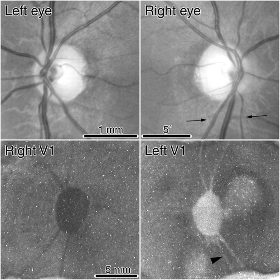
Monkey K. Fundus pictures showing the optic discs and retinal vessels. Below are single CO sections through layer 4C showing the representations of the optic discs pictured directly above. The left eye was enucleated, so the right blind spot representation (represented in the left cortex) appears pale. The thin lines radiating from the blind spot representations are the representations of angioscotomas from shadows cast by retinal vessels leaving the optic disc. Tissue between the arrows is shown in cross section in Figure 5. The leftmost vessel, an artery, is indicated below in the cortex by an arrowhead.

Figure 1.

To detect one's own angioscotomas, close the right eye and stare at the X while holding the page ∼40 cm away. The oval will disappear into your blind spot. Slowly move the page a bit closer or farther away. The black dash above the blind spot will disappear when it falls into the angioscotoma created by your inferior temporal retinal vein. Next, shift your gaze methodically from one letter to the next. As you proceed leftward, you will lose the black dash again. This occurs when it falls in the angioscotoma of the inferior temporal artery.

Geniculate inputs to striate cortex serving the left and right eyes are segregated into stripes within layer 4 that are known as ocular dominance columns (Hubel and Wiesel, 1969, 1977; Horton and Hedley-Whyte, 1984; LeVay et al., 1985). These columns can be labeled by staining the cortex for cytochrome oxidase (CO) activity after enucleation of one eye (Wong-Riley, 1979; Horton and Hubel, 1981; Horton and Hedley-Whyte, 1984). Because CO levels reflect physiological activity, loss of staining occurs in the columns formerly driven by the missing eye. A mosaic of regular, alternating light (enucleated eye) and dark (intact eye) stripes emerges throughout the representation of the visual field, except in two monocular areas: the blind spot and temporal crescent. Columns are absent in these regions because only one eye is represented.

For many years, the squirrel monkey was regarded as an anomaly among primates because it was shown repeatedly to lack ocular dominance columns (Tigges et al., 1977, 1984; Hendrickson et al., 1978; Rowe et al., 1978; Hendrickson and Wilson, 1979; Humphrey and Hendrickson, 1983; Hendrickson and Tigges, 1985; Livingstone, 1996). However, we have demonstrated that ocular dominance columns exist in squirrel monkeys, although they are often quite fine (450 μm per pair in width) and indistinct (Horton and Hocking, 1996b). In this previous study, we failed to locate the representation of the blind spot or the monocular crescent. We now describe these features and in addition show that the representation of a third monocular compartment, the angioscotomas, can be detected using CO in squirrel monkey striate cortex.

This discovery has provided new insight into the physiological basis of angioscotomas. It has also yielded new data concerning the mechanisms underlying the formation of ocular dominance columns and the role of visual experience in the development of the cortex. Finally, it has revealed more clearly the precision of the visual field representation in layer 4C.

Materials and Methods

Experimental animals. These experiments were performed on 12 adult squirrel monkeys (Saimiri sciureus) from an indoor colony at the California Regional Primate Research Center (Davis, CA). All procedures were approved by the University of California San Francisco Committee on Animal Research. Each animal was normal, verified by complete ophthalmological examination under ketamine anesthesia (15 mg/kg, i.m.). During this examination, the ocular fundi were photographed with a model TRC-FE camera (Topcon Medical Systems, Paramus, NJ) mounted on a platform that allowed easy pivoting around the center of the optical axis on the corneal front surface. These photographs were montaged using Photoshop 6.0 (Adobe Systems, San Jose, CA).

After the photographic montages of the fundi were prepared (usually ∼1 week later), each animal was brought back to the laboratory for calibration of the pictures by projection of retinal landmarks onto a tangent screen. Each animal was given ketamine HCl (15 mg/kg, i.m.), intubated, and respirated with 2% isoflorane in a 50:50 mixture of O₂/N₂O. Under general anesthesia the following parameters were monitored continuously: temperature, EKG, heart rate, respiratory rate, tidal volume, end-tidal CO₂, SpO₂, inspiratory and expiratory isoflorane, O₂, and N₂O concentrations. Paralysis was induced with succinylcholine HCl at an infusion rate of 45 mg/kg, i.v.

The animal was placed in a stereotaxic frame mounted on a model 413 professional tripod (Gitzo, Créteil, France). The tripod allowed us to orient the stereotaxic frame to align the eye's visual axis perpendicular to the center of a 6 × 9 foot tangent screen located 57 inches away. The pupils were dilated with 2.5% neosynephrine HCl and 0.125% scopolamine HCl drops. A hard 7.5 mm diameter contact lens was used to prevent corneal drying.

The fundus montage (prepared in advance) was used to select a prominent retinal landmark (e.g., a vessel bifurcation). The landmark was then identified through the fundus camera in the anesthetized, paralyzed animal. The crosshair of the camera was focused on the landmark and locked in place. Next, a mirror was placed flush against the barrel of the objective lens, and the shutter was tripped with the back of the camera open. This reflected a small circle of light back to the tangent screen at a position corresponding to the retinal landmark. With practice, retinal landmarks in the central 30° could be projected with an accuracy of ±0.1°. After plotting ∼15 landmarks, we rechecked the position of the first few to ensure that no eye movements had occurred during the hour required for retinal calibration. Eye movements were rare because of the high dose of succinylcholine used during these brief measurements. The calibration process was repeated in the fellow eye, after the tripod was adjusted to position its optical axis perpendicular to the tangent screen. Positioning the optical axis perpendicular to the tangent screen made it easy to convert distance (χ) on the tangent screen from the foveal projection point to degrees eccentricity (θ) by using the formula θ = arctan χ/57.

After finishing the calibration process for each retina, we enucleated one eye using sterile technique. This procedure was necessary to reveal the angioscotomas (Fig. 1) in the cortex with CO. The animal was then reawakened and returned to its cage. A potent analgesic, Buprenorphine HCl (0.03 mg/kg, i.m.), was given every 8 hr until the animal had recovered completely. In many animals, we recorded from striate cortex for 24 hr before enucleating one eye. These data will be presented in another paper.

Measurements of newborn squirrel monkey eyes. Angioscotoma representations form in striate cortex soon after birth, induced by the shadows cast by retinal blood vessels (Adams and Horton, 2002). To determine the size of these shadows, one must know the diameter (p) of the pupil and the distance (d) from the pupil to the retina in baby monkeys.

In infants, the pupil is smaller, less reactive to light, and less variable in size than in adults (Isenberg et al., 1989; Roarty and Keltner, 1990). To determine the average size of the pupil in baby squirrel monkeys, we took pictures of their eyes using a camera with a ring flash on a 100 mm macro lens. We photographed five babies at age 1 week from the colony at the California Regional Primate Research Center. Pictures were taken in the same housing facility and under the same lighting conditions that were present during the infancy of six animals used in this study (monkeys C, D, E, O, P, Q). No anesthesia (which might affect pupil size) was needed, because squirrel monkeys can be handheld at age 1 week. We allowed plenty of time between flash pictures for the pupil to recover. The mean pupil diameter (p), determined from scanned photographs, was 1.9 mm ± 0.03 mm SEM, n = 10, range 1.7–2.0 mm. Mean corneal diameter was 6.1 mm.

The distance (d) from the pupil to the retina was measured with a Humphrey-Allergan Model 820 A-ultrasound unit (Zeiss Humphrey Systems, Dublin, CA) in three newborn squirrel monkeys. The mean value was 8.4 ± 0.12 mm SEM. Mean axial length was 10.1 ± 0.12 mm SEM.

These measurements provided figures for the size of the entrance pupil and the position of the real pupil in the baby squirrel monkey. Calculation of angioscotoma dimensions depends on the size and position of the exit pupil. Vakkur and Bishop (1963) have compared the diameter of the entrance and exit pupil in the cat eye. They differ by <250 μm for a pupil up to 5 mm in diameter. Therefore, assuming that the squirrel monkey is similar, little error is introduced by measuring the diameter of the entrance pupil rather than the exit pupil. Vakkur and Bishop (1963) also determined the relative positions of the real pupil and exit pupil in the cat eye. They are located within 100 μm of each other for a pupil up to 5 mm in diameter. Thus, location of the real pupil provides an adequate estimate of the location of the exit pupil, at least for our purposes.

To determine the size of a vascular shadow, one must also know the retinal blood vessel lumen diameter (c) and the distance (s) from the blood vessel to the cone inner/outer segment junction. Measurements of these parameters were made in adult eyes that were postfixed in 2% paraformaldehyde and 2% glutaraldehyde, followed by embedding in Epon-Araldite. These procedures induce a mean tissue shrinkage of 18% (Perry and Cowey, 1985). The monkey eye increases in axial length from birth to adulthood by 22% (Smith et al., 2001). Because tissue shrinkage from processing is approximately equal to the growth of the eye from birth to adulthood, dimensions for c and s were taken directly from plastic-embedded adult retinal tissue.

Histological procedures. We waited a minimum of 10 d to maximize changes in cortical CO activity induced by monocular enucleation. We then killed the animals with an injection of sodium pentobarbital (150 mg/kg). Each monkey was perfused through the left ventricle with 1 l of normal saline followed by 1l of 1% paraformaldehyde in 0.1 m phosphate buffer. Flatmounts of striate cortex were prepared from each hemisphere (Horton and Hocking, 1996a), cut with a freezing microtome at 30–40 μm, mounted on slides, air-dried, and reacted for CO. In every animal, the eyes were saved for subsequent histological processing, which included preparation of retinal whole mounts or embedding in Epon-Araldite for semithin sectioning.

Data analysis. Cortical CO flatmounts were imaged at 600 dots per inch on an Arcus II flatbed scanner (Agfa, Mortsel, Belgium) fitted with a transparency adapter to prepare montages of layer 4Cβ. Autoradio-graphs, retina, and high-power cortex pictures were taken with a Spot RT Slider camera (Diagnostic Instruments, Sterling Heights, MI) mounted on an SZH10 (Olympus Optical Co., Tokyo, Japan) or an Axioskop microscope (Zeiss, Thornwood, NY). Images were imported into Illustrator 9.0 or Photoshop 6.0 (Adobe Systems) to prepare the Figures. Measurements were made using CADtools (Hotdoor Inc., Grass Valley, CA) for Illustrator. Adjustments in brightness and contrast were made of individual sections used to assemble cortical montages with Photoshop. In addition, blood vessels were removed using the “dust and scratches” noise filter. It assigned the white pixels in an empty blood vessel lumen to the mean local color value in surrounding cortex. This step removed the distracting profiles of cortical blood vessels from the montages, making it slightly easier to see the angioscotoma representations.

Results

Representation of angioscotomas in striate cortex

Figure 2 shows the optic discs and cortical blind spot representations from monkey K. This animal had only a faint trace of ocular dominance columns, visible in a limited region of the cortex near the monocular crescent representation. No ocular dominance columns were visible in the cortex surrounding the blind spot representations. By the term “blind spot” representation, we are referring to a region of cortex corresponding to the visual field location of the blind spot. For example, the blind spot of the left eye is represented in the right cortex, and it receives input derived exclusively from the right (ipsilateral) eye.

Figure 2 shows raw data, namely, single cortical sections before application of the dust and scratches filter and the preparation of montages. The sections pass mostly through layer 4Cβ but graze deeper layers. The blind spot representation in the right cortex appeared dark, because it was supplied solely by the remaining right eye. Conversely, the blind spot representation in the left cortex was pale, because the left eye was enucleated.

In the right cortex, approximately eight thin dark threads radiated out from the blind spot representation of the left eye. These were the cortical representations of angioscotomas created by blood vessels emanating from the left optic disc. They were dark, like the blind spot representation, because they received input only from the intact right eye. In the left cortex, the representations of the angioscotomas were also visible; however, they were pale rather than dark, because their input derived exclusively from the enucleated left eye. Fewer angioscotomas are visible in this section because portions skimmed layer 5.

The angioscotomas were seen best in layer 4Cβ. They were also present in layer 4Cα, but lower in contrast. They could not be detected in any other cortical layer. Figure 3A shows the array of CO patches in layer 3. No hint of the angioscotomas or the blind spot representation was apparent. Moreover, the trajectory of the angioscotomas in layer 4Cβ bore no relationship to the CO patches in other layers (Fig. 3B). In layer 4A (Fig. 3C), the blind spot representation was slightly darker than surrounding cortex, but no angioscotomas were seen. In layer 5 (Fig. 3D), neither the blind spot nor the angioscotomas were seen.

Figure 3.

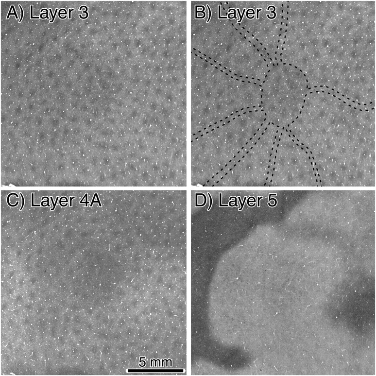
Monkey K. A, Single section of layer 3, cut through the same region of the right cortex shown in Figure 2 (see bottom left panel) but 210 μm more superficial. CO patches are present throughout the area. No effect of monocular enucleation is visible. The blind spot representation is not apparent, because the upper layers in squirrel monkey contain highly binocular cells. B, Same section as in A, with the locations of the blind spot and angioscotomas from layer 4 outlined with dots. The patches neither skirt nor follow the path of the angioscotomas. C, Single section grazing layer 4A, immediately adjacent to the section shown above. The region overlying the blind spot representation appears slightly darker than surrounding cortex, but the angioscotomas are not visible. D, Single section cut mostly through layer 5, 105 μm below the section shown from layer 4C in Figure 2, bottom left. No hint of the blind spot or angioscotomas is seen.

These findings highlight a fundamental difference between the organization of striate cortex in macaque monkeys and squirrel monkeys. In macaques, the patches outside layer 4C are organized in rows aligned with an ocular dominance column (Horton and Hubel, 1981; Horton, 1984). Because patches are aligned with ocular dominance columns and receive a monocular konio-cellular input (Hendry and Yoshioka, 1994; Horton and Hocking, 1996a, 1997), their cells tend to be monocular (Livingstone and Hubel, 1984). Consequently, after monocular enucleation the rows of patches in register with columns of the missing eye turn pale. The blind spot representation becomes visible in every layer because ocular dominance is perpetuated outside layer 4C (Fig. 4). However, its contrast is lower outside layer 4C because the segregation of ocular inputs is weaker.

Figure 4.

Macaque monkey. A, Single CO section through layer 4C, after enucleation of the contralateral eye. This experiment was done in connection with an unrelated project and is shown here simply for comparison with Figure 2, bottom left panel. The blind spot representation appears dark, as in the squirrel monkey. The striking difference is that the surrounding cortex is organized into high-contrast, large, sharply defined ocular dominance columns. B, Section from the same region, 315 μm more superficial, passing through layer 3. The patches in every other row appear pale, as opposed to the squirrel monkey, in which all patches retain the same level of CO activity after monocular enucleation. In addition, the blind spot representation is visible as an oval dark zone matching its shape in layer 4C. The blind spot representation is visible in all layers because the cortex outside layer 4 retains greater monocularity than in the squirrel monkey.

In the squirrel monkey, the patches have no relationship to ocular dominance columns in layer 4. All patches in the upper layers are labeled after a tracer injection into one eye (Horton and Hocking, 1996b). Their cells are far more binocular than those in the macaque (Livingstone and Hubel, 1984). Consequently, after monocular enucleation, the blind spot representation can be seen in CO sections of layer 4 but not other layers. The CO levels in other layers are maintained by activity driven by the remaining eye. This means that the retinotopic map must be quite coarse outside layer 4, because inputs from the remaining eye are imported from outside its blind spot representation. Our CO data therefore support the evidence from physiological recordings that receptive field size and scatter are greater in layers outside 4C (Hubel and Wiesel, 1974). The precision of retinotopic organization is likely to be similar in the upper layers of squirrel monkey and macaque cortex. Therefore, the visibility of the blind spot outside layer 4C in macaques is probably caused mainly by stronger monocularity.

Shadows cast by retinal blood vessels

Figure 5 shows a 1 μm cross section from the right eye of monkey K that extends between the two arrows in Figure 2. The section contains two prominent arteries, flanking a vein, in the nerve fiber layer. Large retinal vessels emanating from the optic disc pass directly into the nerve fiber layer. They descend into the ganglion cell layer as their distance from the optic disc increases (Snodderly and Weinhaus, 1990; Snodderly et al., 1992). In the ganglion cell layer they create channels, disrupting the normal cellular architecture. This can be seen in Figure 5 by tracing the path of the small tributary to the big vein, which enters the ganglion cell layer. In the vicinity of this venous branch, the ganglion cells have been displaced. One might propose that gaps in the ganglion cell layer from blood vessels give rise to angioscotomas. This idea is dispelled by the large artery in Figure 5 located above the ganglion cell layer. It produced an angioscotoma in the cortex (Fig. 2) but no disruption of the ganglion cell layer beneath it. Therefore, physical displacement of ganglion cells by blood vessels is not responsible for angioscotomas.

Figure 5.

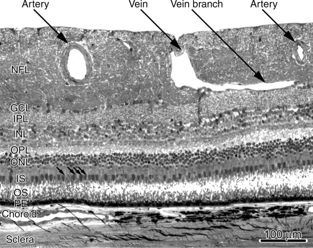
Monkey K. Plastic section (1 μm) of the right eye, stained with Toluidine blue, passing between the arrows shown in Figure 2. The precise location was pinpointed by the junction between the vein and its branch, which can be seen in the retinal photograph, although it is a bit out of focus. Near the optic disc, large vessels are situated in the nerve fiber layer, which becomes especially thickened. The vein branch enters and disrupts the ganglion cell layer. The artery on the left, the angioscotoma representation of which is marked by an arrowhead in Figure 2, has a lumen diameter of 57 μm. This was calculated by measuring the lumen circumference and dividing by π (we assumed the oval shape was a postmortem artifact). The small arrows denote four ellipsoids of cone inner segments, located underneath the artery. NFL, Nerve fiber layer; GCL, ganglion cell layer; IPL, inner plexiform layer; INL, inner nuclear layer; OPL, outer plexiform layer; ONL, outer nuclear layer; IS, inner segments; OS, outer segments; PE, pigment epithelium.

Angioscotomas arise from light absorption by hemoglobin within red blood cells, resulting in a shadow cast on photoreceptors beneath. The blood vessel wall is virtually transparent to light. Therefore, only lumen diameter is pertinent to the following optical calculations. Figure 6A shows a schematic drawing with rays of light traced from the edge of the pupil to a retinal vessel. Any object (e.g., a retinal vessel) illuminated by a non-point source (e.g., the pupil) creates a shadow composed of a central umbra surrounded by a penumbra (Fig. 6B). The width of these shadows depends on four variables: p = exit pupil diameter; d = distance from exit pupil aperture to retinal blood vessel; s = distance from blood vessel to the junction between cone inner/outer segments; c = retinal blood vessel lumen diameter.

Figure 6.

A, Schematic scale drawing of the squirrel monkey eye illustrating the paths of light from the pupil to the retina. The dimensions used to calculated the size of shadows cast by retina blood vessels are labeled: p, pupil diameter; d, pupil aperture to blood vessel distance. B, The boxed region of retina from A shown at higher magnification. The rays of light are shown superimposed onto a 1 μm plastic section of squirrel monkey retina. A single artery of lumen diameter c is present in the retinal ganglion cell layer at a distance s from the photoreceptor inner/outer segment transition plane (the shadow plane). The shadow cast by this vessel comprises a central total shadow (umbra) bordered by a peripheral partial shadow (penumbra).

Mean pupil diameter (p) was 1.9 mm and mean distance from the exit pupil to the retina (d) was 8.4 mm (see Materials and Methods).

The distance s was sampled in 1 μm plastic cross sections throughout the retina from three fixed adult specimens. Figure 7A shows a series of aligned sections, which are stacked to show retinal blood vessels in cross section from the fovea to the optic disc. One can identify individual vessels in the fundus photograph and find their corresponding cross section in the 1 μm plastic sections to determine s and c at any point (Fig. 7C,D). For vessels visible in the photograph, s ranged between 165 and 253 μm. In the macula, s was large because the ganglion cell and Henle fiber layers were thick. Near the optic disc and along the major vascular arcades, s was large because the nerve fiber layer was thick. In peripheral nasal retina, s was small because the retinal layers were thin; it measured only 115 μm at 50° (angioscotomas were visible rarely in the cortex beyond this eccentricity).

Figure 7.

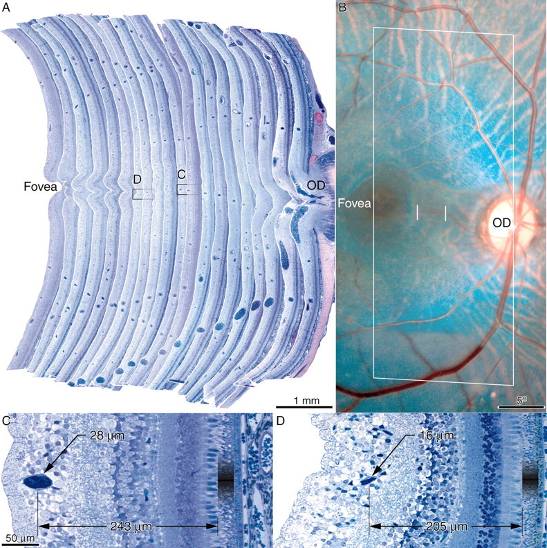
Monkey Q, right retina. A, Stacked series of 20 plastic cross sections (1 μm), each 125 μm apart, compiled to measure s (distance from center of blood vessel lumen to cone inner/outer segment junction) for individually identified vessels at different locations. Boxed vessel is shown in panels below. B, Photograph of right fundus, outlining the retina illustrated histologically (A) with a rectangle. The fine vertical white lines indicate the positions of cross sections shown below. C, High-power view of venule only 28 μm in lumen diameter (calculated assuming circular cross section), the representation of which was visible in the cortex. The vessel was located at an eccentricity of 7.5° and cast only penumbra, equal to 83 μm (gradient between thin black lines), on the basis of values s = 243 μm, p = 1.9 mm, d = 8.4 mm. D, The same venule, but at an eccentricity of 4.1°, cast only penumbra, measuring 64 μm, on the basis of the indicated parameters. This shadow did not induce a visible representation in the cortex. OD, Optic disc.

The width of vessel shadows can be calculated using similar triangle geometry in Figure 6 (Applegate et al., 1990):

Figure 8A is a graph of vessel diameter versus shadow width calculated from the above formulas using fixed values of s = 200 μm, d = 8.4 mm, and four different pupil diameters. The shadow contains two components: the umbra (solid line) and the penumbra. Total shadow width (dotted line) equals the umbra plus twice the penumbra. The graph provides shadow widths cast by blood vessels of various lumen diameter. For example, a vessel of diameter 40 μm illuminated through a 1.0 mm pupil casts a shadow 65 μm wide, the umbra of which occupies the central 17 μm. If the vessel is small enough, or the pupil large enough, the shadow will consist of penumbra alone. For example, the same 40 μm diameter vessel illuminated through a 3 mm pupil will cast no umbra on the photoreceptors but will cast a penumbra measuring 111 μm wide.

Figure 8.

A, Graph showing the widths of shadows cast onto photoreceptors by retinal vessels of different lumen (c) at various pupil diameters (p). Solid lines represent the width of the umbra alone, and dotted lines represent the width of the whole shadow (umbra + twice penumbra). Pupil diameters of 1, 3, and 4 mm are shown, plus 1.9 mm, the experimentally determined value for an infant squirrel monkey. The values of s and d were 200 μm and 8.4 mm, respectively. B, Graph showing the widths of shadows cast onto photoreceptors by retinal vessels of different lumen (c), at various distances (s) from the photoreceptor layer. Solid lines represent the width of the umbra alone, and dotted lines represent the width of the total shadow. Five values of s are shown: 100–300 μm. For this graph, p and d were fixed at 1.9 and 8.4 mm, respectively.

Figure 8A shows shadow widths for a pupil diameter of 1.9 mm, the mean pupil size in infant squirrel monkeys, as well as for diameters of 1.0, 3.0, and 4.0 mm. From inspection of the graph, it is evident that most vessels in the ganglion cell layer of the infant monkey cast only a penumbra on photoreceptors. In fact, vessels <44 μm in diameter cast no umbra when the pupil diameter equals 1.9 mm. Only the largest vessels, which form the main vascular arcades of the retina, give rise to an umbra. For example, the large artery in Figure 5 (and Fig. 2, top right panel) has a lumen diameter of 57 μm, producing an umbra of 13 μm and a total shadow of 104 μm.

With spontaneous changes in pupil diameter, shadows from blood vessels will fluctuate in size and density. As described in a later section, the representation of vessels with a lumen as small as 28 μm can be detected in the cortex. An umbra forms transiently under such small vessels only during moments of extreme pupil constriction. Therefore, we suspect that in many cases penumbra alone is sufficient to induce an angioscotoma representation in the cortex.

The minimum vessel size of 44 μm for umbra formation calculated above used a value of 200 μm for the distance (s) from the blood vessel to the photoreceptor layer. Because s is a critical factor, we plotted shadow width as a function of s, setting pupil diameter (p) to 1.9 mm (Fig. 8B). Measurements in retinal cross sections from three animals revealed that s is never <150 μm for retinal blood vessels in the central 24°, whose angioscotomas are visible in the cortex. For p = 1.9 mm, s = 150 μm, the smallest vessel casting an umbra would have a lumen of 33 μm. As noted above, smaller vessels are represented in the cortex. These calculations, based on conservative values for p and s, confirm that many angioscotomas are induced by penumbra, without umbra.

We propose that angioscotoma representations are generated by the same process that leads to shrinkage of ocular dominance columns after early monocular eyelid suture or cataract (Hubel et al., 1977). The penumbras (and occasionally umbras) of blood vessels that fall on photoreceptors cause local deprivation in the retina, leading to remodeling of geniculocortical afferents during the critical period. After enucleation in the adult animal, the blind spot and the angioscotomas are revealed by CO.

According to this hypothesis, angioscotomas mapped in adults do not arise from vascular shadows (although they were induced by them during childhood) but represent a secondary phenomenon from amblyopia. This would explain why angioscotomas tend to be wider than the diameters of the blood vessels themselves (Remky et al., 1996). If one could somehow make an adult's retinal vessels transparent, angioscotomas would persist. This conclusion leads one to predict that angioscotoma width in adults does not depend directly on pupil size. Once the retina has become amblyopic, angioscotoma width should be fixed and hence independent of the width of the inducing shadow. If the pupil were made large (by instillation of mydriatic drops), blood vessels would throw large, weak penumbras on the retina. Nevertheless, angioscotomas would remain discrete and dense, because they correspond to a zone of “amblyopic” photoreceptors, not a vascular shadow. Extreme constriction of the pupil, however, might create an umbra even wider than the angioscotoma defined by amblyopic photoreceptors.

Mapping angioscotoma representations in striate cortex

Figure 9 shows the angioscotoma representations in the right cortex of monkey L. This animal had rudimentary ocular dominance columns. The montages of layer 4C were slightly uneven because of seams from the montaging process and fluctuations in CO density with varying depth in layer 4Cβ. The near absence of columns in monkey L was genuine rather than a failure of CO staining, because CO readily labeled the blind spots and angioscotomas. Successful labeling of these monocular zones means that if ocular dominance columns had been present, CO would have revealed them.

Figure 9.

Monkey L, right hemisphere. A, CO flatmount montage, showing dark blind spot and angioscotoma representations after enucleation of the left eye. Except for some fluctuations in CO density near the monocular crescent, ocular dominance columns were essentially absent in this animal. B, Photomontage of the left fundus. C, Drawing of angioscotomas. D, Drawing of retina, with color-coded vessels represented in the cortex.

The angioscotoma representations were thinnest in animals with rudimentary columns, as in monkey L or monkey K (Fig. 2). Their pattern was drawn by eye (Fig. 9C) to estimate their total area and perimeter. In the right cortex of monkey L, the angioscotomas had an area of 20.8 mm² and a perimeter of 240.6 mm. Mean angioscotoma width, obtained by dividing the area by half the perimeter, was 172 μm. In the left cortex, the angioscotomas had an area of 13.1 mm² and a perimeter of 148.7 mm. These values yielded a mean angioscotoma width of 176 μm.

In monkey Q, the next animal, the ocular dominance columns were better developed than in monkey L (Fig. 10A, compare with Fig. 9A). Nonetheless, they were too indistinct to draw accurately. To gain an impression of their periodicity, the spatial Fourier spectrum of the CO montage was analyzed using Matlab 5.0 (Math-works, Natick, MA). The power spectrum had a peak at 1.94 cycles per millimeter, corresponding to a single column width of 258 μm. For the sake of illustration, we bandpass filtered the CO montage (Fig. 10A) to create a pattern similar in periodicity to the ocular dominance columns. This pattern was used to provide the background columns in the schematic drawing of the cortical angioscotomas (Fig. 10C).

Figure 10.

Monkey Q, right hemisphere. A, Layer 4C CO montage, showing blind spot with 12 radiating angioscotoma representations. They are pale because the right eye was enucleated. The angioscotomas are particularly extensive and obvious in this animal. A fine pattern of rather indistinct ocular dominance columns is present. B, Retinal montage, compiled from fundus pictures taken in vivo. C, Color-coded drawing of angioscotomas visible in A. A few angioscotomas of reversed (dark) CO contrast, induced by vessels in the temporal retina of the right eye, are shown in black. D, Drawing showing 12 vessels in nasal retina represented in the right cortex.

Monkey Q had an unusually clear and complete pattern of cortical angioscotomas. They appeared so extensive, as we propose in the next few pages, because the periodicity of the animals' ocular dominance columns was ideal for their visualization. In monkey Q's right cortex, the angioscotomas had an area of 55.3 mm², a perimeter of 358.1 mm, and a width of 310 μm. In the left cortex, the angioscotomas had an area of 82.2 mm² and a perimeter of 528.7 mm, yielding a mean angioscotoma width of 310 μm. Compared with monkey L, the angioscotomas were much wider (310 vs 174 μm) and more fully represented.

Monkey E (Fig. 11) had clearly defined ocular dominance columns throughout striate cortex in both hemispheres. The columns were coarser than those in monkeys L and Q. Fourier analysis yielded an average single column width of 452 μm. Representations of only a few of the largest fundus vessels were visible. Combining data from both hemispheres, we found that the angioscotoma representations occupied just 36 mm². They had a mean width of 344 μm.

Figure 11.

Monkey E, right hemisphere. A, CO flatmount montage, showing dark blind spot and angioscotoma representations after enucleation of the left eye. A pattern of “intermediate” ocular dominance columns can be seen throughout the cortex except in the representation of the blind spot and monocular crescent. Only the largest blood vessels are represented within the ocular dominance mosaic. B, Single fundus photograph including the optic disk, major retinal vessels, and fovea. C, Drawing of angioscotomas. Dotted line represents striate cortex corresponding to the extent of the fundus photograph. D, Drawing of retina, with color-coded vessels represented in the cortex. Star, Fovea.

Monkey N had well segregated ocular dominance columns (Fig. 12). For a squirrel monkey, they were extraordinarily large. Mean single column width by Fourier analysis was 608 μm. No representations of retinal blood vessels were recognizable in the cortex; however, the blind spot and monocular crescent representations were seen easily.

Figure 12.

Monkey N, right cortex. A highly segregated pattern of coarse ocular dominance columns (reminiscent of macaque and human striate cortex) precludes the formation of angioscotoma representations.

Among normal squirrel monkeys, there is enormous inherent variability in the expression of ocular dominance columns (Adams and Horton, 2003a). In some animals, like monkey K (Fig. 2) or monkey L (Fig. 9), they were nearly absent. In other animals, such as monkey N (Fig. 12), they were as prominent as those found in macaques and humans. The 12 monkeys in this study could be grouped into four categories on the basis of the appearance of their ocular dominance columns. This was useful for illustration of our data, but we do not mean to suggest that such discrete categories exist in nature. Four monkeys (I, J, K, L) had rudimentary columns, and four (C, M, P, Q) had fine (∼250 μm wide), rather indistinct columns. Two monkeys (D, E) had medium (∼450 μm wide), well defined columns, and two (N, O) had large (∼600 μm), highly segregated columns. A consistent relationship was found between the visibility of angioscotomas and the periodicity of ocular dominance columns. Figure 13 shows schematically the influence of column periodicity on the appearance of angioscotoma representations.

Figure 13.

Schematic illustration of the relationship between ocular dominance column periodicity and angioscotoma visibility in the cortex. The pattern of geniculate afferents from the left and right eye is represented as black and white. The region of striate cortex shown here contains the superior half of the blind spot representation. The four panels show examples of different column periodicities: A, rudimentary columns (monkeys L, K); B, fine columns (monkeys C, Q); C, intermediate columns (monkey E); D, coarse columns (monkey N). Note that angioscotomas are best seen in animals with fine columns, because they are highlighted by columns serving the other eye. Angioscotomas are not well seen in animals with coarser, better segregated columns, because the columns override the angioscotoma pattern.

In animals with rudimentary columns, the width of angioscotoma representations is a faithful reflection of shadow width, shadow density, and local cortical magnification factor. In animals with better developed ocular dominance columns, the situation is more complex. Assume that ocular dominance columns in squirrel monkey, when they occur, are present at birth, as they are in macaques. Under these circumstances, ocular dominance columns must be remodeled in the cortex for angioscotomas to become visible. Territory belonging to the eye in which photoreceptors are obscured is taken over by the eye that has an unencumbered view of the visual scene. Consequently, solid channels develop, cutting swaths through the mosaic of ocular dominance columns. Enucleation reveals the angioscotomas because they are tantamount to remodeled ocular dominance columns. These remodeled ocular dominance columns are centered on the retinotopic position of retinal blood vessels but are not necessarily equal to their retinotopic width.

Because angioscotoma representations are simply ocular dominance columns, their width appears to be strongly influenced by the inherent periodicity of the ocular dominance columns present in any given animal. The angioscotoma representations are wider in animals with fine or intermediate columns (Figs. 10, 11) than in animals with rudimentary columns (Fig. 9). Their enhanced width makes them easier to detect. This helps explains why more of the retinal vascular tree is represented in monkey Q than in monkey L. It appears that the cortex strings together “pixels” about the size of ocular dominance columns to create the angioscotoma representations.

As the periodicity of columns increases beyond an optimal range (200–300 μm single column width), fewer and fewer retinal blood vessels are represented. In monkey E (Fig. 11), an animal with a mean column width of 450 μm (calculated from the peak in the spatial Fourier spectrum of the CO montage), only the largest retinal vessels were represented. They appeared similar to the underlying mosaic, and in many places, their paths became disrupted by the column pattern. In monkey N, whose mean column width was 608 μm, no angioscotomas could be discerned at all (Fig. 12). We suspect that in such animals columns are unable to remodel to form angioscotoma representations. This may reflect the tendency for larger columns to be better segregated. In such animals, greater “repellency” between the geniculocortical afferents serving the two eyes may render it impossible for the afferents of one eye to carve a narrow channel (corresponding to an angioscotoma) through a large ocular dominance column serving the other eye.

In animals with fine or intermediate columns, the cortical angioscotoma representations were flanked by zones of opposing contrast, producing an optical density profile resembling an inverted Mexican hat (Adams and Horton, 2002). The presence of this “frosting” of opposite contrast served to highlight angioscotoma representations, rendering them more obvious. This explains in part why the angioscotomas were so apparent in monkey Q.

Why are the angioscotoma representations flanked by zones of opposite contrast in monkeys with fine columns? In such animals, an angioscotoma representation consists of a continuous channel created by remodeled ocular dominance columns. As explained previously, this channel is larger than the retinotopic width of the vessel. Consequently, the angioscotoma representation also incorporates slivers of visual field flanking the blood vessel. To balance the local representation of each eye, the angioscotoma representation becomes bracketed by cortex serving the other eye. This means, essentially, that an exchange of cortical territory must occur during early development. One eye takes over a solid swath of territory, corresponding to the location of the blood vessel of the other eye, plus some surrounding visual field. In return, it abandons all territory along a strip flanking either side of the angioscotoma representation.

In animals with rudimentary columns, the angioscotoma representations faithfully represent the amblyogenic width of shadows cast by retinal vessels. They are not flanked by columns serving the other eye. Consequently, they are more difficult to detect in the cortex, because of the lack of “highlighting” by the other eye and their finer caliber. Animals with fine columns, like monkey Q, have the most extensive pattern of cortical angioscotomas because their columns amplify the width of the angioscotomas and create a frosting effect. Animals with large columns (Figs. 11, 12) have fewer cortical angioscotomas because their columns are less capable of remodeling. Thus, there is an optimal width of ocular dominance column (∼250 μm wide) in the squirrel monkey that results in maximum visibility of angioscotomas in the cortex.

Precision of the cortical retinotopic map

The retinal vascular tree is transformed by cortical magnification (M) to form the pattern of angioscotoma representations in the cortex. The largest vessels in the squirrel monkey retina are the arteries and veins emerging from the optic disc. They follow an arcuate course into the temporal fundus, maintaining an eccentricity of ∼15°. Consequently, their cortical representations follow a fairly straight course from the optic disc representation to the V1/V2 border (vertical meridian representation). Along their arcuate course, the caliber of the largest retinal vessels remains quite constant. Because their diameter and eccentricity change little, their cortical representations also remain quite constant in width.

As retinal vessels branch toward the fovea, they rapidly diminish in caliber. Their taper is offset by a rise in M, maintaining cortical angioscotomas at a fairly constant width. At an eccentricity of 4–5°, however, angioscotoma representations disappear abruptly in the cortex. Do they vanish because retinal vessels become too thin to cast an amblyogenic shadow or because their cortical representations become too small to see?

To address this issue, we determined the expected width of the cortical representation of vessels coursing toward the fovea. For example, the penumbra of the vessel featured in Figure 7, C and D, was calculated to be 83 μm at 7.5° and 64 μm at 4.1°. In the squirrel monkey the equation for M along an isoeccentricity ring is M_e = 188(6.45 + E)^-1.85, where E = eccentricity in degrees (Adams and Horton, 2003b, their Fig. 4). Determination of M along this dimension is appropriate because the vessel is oriented radially to the fovea. Application of the formula yields 1.43 mm/° at 7.5° and 2.41 mm/° at 4.1°. The retinal magnification factor in squirrel monkey central retina is 161 μm/° (Adams and Horton, 2003b). Accordingly, the predicted width of the angioscotoma representations are 737 μm at 7.5° and 958 μm at 4.1°. Thus, if angioscotoma representations were simply a reflection of M, they would increase in width toward the foveal representation. The fact that they disappear leads one to conclude that retinal vessels eventually become too thin to cast a shadow sufficiently dense to induce remodeling of geniculocortical afferents. Parenthetically, we note that 737 μm is far greater than the actual width of the angioscotoma representation in the cortex at 7.5°. This point is discussed below.

As vessels flow into peripheral nasal retina, they become smaller; in addition, M diminishes. Therefore, few angioscotomas are represented in the cortex at eccentricities >30°. Only a single animal, monkey Q, had angioscotoma representations that reached the monocular crescent (Adams and Horton, 2002, their Fig. 4).

Thus two distinct phenomena conspire to concentrate angioscotoma representations in a belt of cortex extending from 5° to 30°. At <5°, shadow contrast is too low to deprive retinal photoreceptors. At >30°, vessel size and M are too small to create a cortical representation large enough to be detected with CO. Between 5° and 30°, vessel diameter and M are balanced to produce angioscotomas of quite constant width.

The largest vessels represented in the cortex are the veins that emanate from the optic disc. They attain a diameter in squirrel monkey retina of nearly 100 μm (0.62°). What is the smallest retinal vessel represented in the cortex? As discussed in the previous section, angioscotoma representations are a direct product of shadow width only in animals with rudimentary ocular dominance columns. To answer this question, therefore, we examined monkey K, an animal with virtually no ocular dominance columns. Figure 14 shows the cortical representation of a venule in the left retina. It was one of the smallest vessels with a detectable cortical representation in this animal. Because the venule crossed a prominent artery, its location could be pinpointed in the retinal whole mount. It had a lumen diameter of 30 μm, corresponding to 11.2 min of arc, at an eccentricity of 12.5°. The cone outer segments in this portion of the retina had a diameter of 7–8 μm. Therefore, the vessel, when projected directly onto the cone mosaic, had a width of approximately four cones (Fig. 14E); it cast, of course, a much wider shadow. The vessel lumen was centered 180 μm above the cones. Inserting values of s = 180 μm, c = 30 μm into the graph in Figure 8B yields a shadow 72 μm (0.45°) in width that consists entirely of penumbra.

Figure 14.

Monkey K. A, Diagram showing vessels represented in cortex of monkey K, an animal with only rudimentary ocular dominance columns. A photograph of the left optic disc is shown in Figure 2. The boxed region is shown in C. B, Diagram showing the angioscotomas visible in the right cortex, color-coded to vessels in A. The angioscotomas near the optic disc are shown in Figure 2. C, View of a small venule (red arrows) crossing the inferotemporal artery at an eccentricity of 12.5°. D, Single CO-stained section, showing representation of the venule, which measured 102 μm in the cortex. E, Photomicrograph of the unstained retinal whole mount, showing the boxed region in C where the venule crosses the artery. At this location the venule had a lumen diameter of 30 μm. The cobblestone pattern of cones is shown for comparison with the size of the blood vessels. This figure was prepared by photographing the retinal layers containing the cones and vessels separately. Photoshop 6.0 was then used to superimpose the vessels on the cone mosaic. Cones underneath the blood vessels are obscured by red cells. F, Graph showing the fraction of pupil occlusion as a function of distance on the retina from the center of the penumbra cast by the venule in E. The shadow eclipsed a maximum of 86% of the pupil. The central 20 μm (between vertical dashed lines) of the 72 μm penumbra had sufficient contrast to produce a representation in the cortex, corresponding to an amblyogenic threshold of 66% pupil occlusion. Pupil occlusion is illustrated schematically by red vessel eclipsing gray pupil at five different positions.

Applying the formula for M_e, one can determine that a shadow 0.45° wide at 12.5° eccentricity will produce an angioscotoma representation 364 μm wide in the cortex. In fact, the angioscotoma representation measured only 102 μm across (Fig. 14D). This discrepancy indicates that only the central portion (102/364 μm = 28%) of the shadow was dense enough to cause remodeling of geniculocortical afferents and hence to become represented in the cortex. This corresponds to the central 20 μm (20/72 μm = 28%) of the shadow. Figure 14F shows the density profile of the penumbra cast by this vessel. In this example, the vessel eclipsed a maximum of 86% of the pupil. At 10 μm from the shadow center, where the vessel eclipsed only 66% of the pupil, the shadow density fell below the threshold required to induce a cortical representation. In terms of optical density, a shadow ranging between 0.85 and 0.45 log units was required to cause amblyopia.

Angioscotoma representations are smaller than the visual angle subtended by the vessel shadow, because only the densest central portion of the shadow is amblyogenic. The proportion of the shadow represented in the cortex varies according to s, d, p, and c. It also depends on the shadow contrast required to induce deprivation. It is unknown whether this “amblyogenic threshold” varies throughout the retina. To address this point, the analysis was repeated for five other vessels at points that could be located reliably by vessel crossings or bifurcations (Table 1). A wide range of blood vessel diameters (30–78 μm) and eccentricities (12.5–20°) was sampled. Some of the blood vessels measured were sufficiently large and close enough to the photoreceptor layer to cast an umbra, whereas others were not. The amblyogenic threshold showed a narrow range, between 52 and 66% pupil eclipse.

Table 1.

Pupil occlusion (amblyogenic threshold) corresponding to edges of the representations of six retinal vessels in monkey K

	Retinal measurements					Shadow widths
Hemisphere	Eccentricity (E)	Lumen diameter (C) μm	Distance to PRs (s) μm	Umbra μm	Total μm	Amblyogenic threshold %
Right	12.5°	30	180	0	72	66%
Right	12.5°	50	180	9	93	65%
Left	19.0°	78	190	35	124	65%
Left	16.5°	66	198	21	113	66%
Left	20.0°	36	208	0	85	52%
Left	13.5°	30	213	0	80	60%
						Mean 63% ± 3% SD

Eccentricities were taken from calibrated fundus pictures. Lumen diameter and distances to photoreceptors (PRs) were measured either from 1 μm sections or from a retinal whole mount. Shadow widths were calculated (see Results) and compared with the widths of cortical angioscotomas to find the amblyogenic threshold. A mean of 63% of the pupil aperture had to be eclipsed for remodeling of geniculocortical afferents. Underlined values are illustrated in Figure 14.

For the 30 μm venule in Figure 14, only 20 μm of the shadow was represented in the cortex. The cones in the vicinity of the venule (located at 12.5°) had a diameter of 6–7 μm. Thus, the visuotopic map in layer 4C is sufficiently precise to resolve patterns of CO activity created by amblyogenic shadows just three cones wide. The true grain of the map is probably even finer and may approach the discrete representation of individual cones.

Another measure of the fidelity of the cortical map can be derived by examining the representation in layer 4C of closely spaced retinal vessels. Figure 15 shows the representation of the superior artery and vein in the left retina of monkey C. As the vessels emerge from the optic disc and course along the retina, their separation gradually increases. At the top of Figure 15 (∼8° from the optic disc), each vessel is distinctly represented in the cortex. As one follows the retinal vessels back to the optic disc, they become closer together but remain discrete; however, their cortical representations merge ∼2 mm above the optic disc representation. At the merger point, the centers of the vessel representations are separated by 340 μm. Thus, in layer 4C, the retinotopic resolution of squirrel monkey striate cortex is 340 μm. This value is an upper estimate, of course, because it may reflect a limitation of the CO technique. At the merger point, the centers of the artery (0.45° width) and vein (0.59°) were separated by 0.65°. This value is probably quite close to the aggregate receptive field size at this eccentricity.

Figure 15.

Monkey C. A, Upper pole of the left optic disc, showing an emerging superior retinal artery and vein. The vessels (blue arrowheads) remain completely separate along their retinal course. B, Corresponding region from the right striate cortex, showing the cortical representation of the vessels in layer 4C (blue arrowheads). They merge ∼2 mm above the optic disc representation. At this point, the centers of the retinal vessels are 0.65° apart and their cortical representations are 340 μm apart.

Previously, deoxyglucose and optical imaging have been used to derive estimates of cortical resolution (Tootell et al., 1988; Grinvald et al., 1994). Blasdel and Campbell (2001) obtained a value of 1200 μm in macaque striate cortex. This figure reflects the fact that optical images are derived mostly from the upper layers, where neurons have greater retinotopic scatter in receptive field position.

Discussion

Helmholtz discovered 135 years ago that scotomas corresponding to the Purkyně retinal tree can be plotted in the visual field. We now show that these scotomas can be detected in striate cortex.

The representation of angioscotomas in V1 provides an intriguing glimpse of the role played by visual experience in the development of the cortex. Its development proceeds according to an innate plan, which is refined by sensory stimulation after birth. Ocular dominance columns provide a classic example of this interplay between genetic instructions and visual experience. Their formation occurs without visual experience (Horton and Hocking, 1996a; Crowley and Katz, 1999, 2000), but they are still indistinct at birth (Rakic, 1977). Several weeks of postnatal life are required for their complete segregation (LeVay et al., 1978, 1980). In the cat, dark-rearing results in poor segregation of columns, demonstrating that visual experience is vital during these postnatal weeks (Swindale, 1981; Mower et al., 1985). In the macaque, the effect of dark-rearing from birth has never been tested. One might find perfectly segregated columns, because the innate drive for column formation is so powerful in this species. Whatever the case, many experiments have provided abundant evidence that visual experience is necessary for normal maturation of geniculocortical afferents, columnar systems, receptive field properties, and visual function (Wiesel and Hubel, 1965; Sherman et al., 1974; Blakemore and Van Sluyters, 1975; Freeman et al., 1981; Swindale, 1988; Movshon and Kiorpes, 1990; Crawford et al., 1991; Blasdel et al., 1995; Antonini and Stryker, 1998; Crair et al., 1998; Hübener, 1998; White et al., 2001).

Amblyopia supplies a classic example of how visual experience can influence the development of the cortex. Kittens and monkeys raised with monocular eyelid suture, to simulate congenital cataract, show expansion of the columns serving the open eye at the expense of those belonging to the deprived eye (Hubel et al., 1977; Shatz and Stryker, 1978; LeVay et al., 1980; Wiesel, 1982; Horton and Hocking, 1997; Schmidt et al., 2002). This result proves that the competition for synaptic connections with cells in layer 4C can be biased toward one eye by handicapping the other eye. However, in these studies the handicap to one eye is global and arises by means of an artificial manipulation that never occurs as part of normal development.

Our finding that angioscotomas are represented in the brain allows one to generalize from observations in lid-sutured animals to the process of cortical development in normal animals. In some squirrel monkeys, ocular dominance columns are so weakly expressed that vascular shadows have an unfettered ability to rearrange geniculocortical afferents. In these cases, the narrow channel carved through the cortex reflects faithfully the “amblyogenic threshold” of the shadow (Fig. 14F). In other animals, with better developed columns, shadows also induce rearrangement of geniculocortical afferents but do so by reallocating units approximately the size of ocular dominance columns. The angioscotoma representations thus appear widened, or amplified, because they subtend more visual field than the amblyogenic portion of the blood vessel shadow. Remarkably, they become surrounded on either side by columns serving the other eye. This frosting makes the angioscotomas more conspicuous in cortical flatmounts. The frosting phenomenon arises, we suspect, because the ocular dominance columns possess an intrinsic periodicity. Vascular shadows perturb the local balance of neural activity in the cortex, tipping column formation in favor of one eye. The other eye is compensated by reciprocal assignment of the nearest adjacent cortex. Such mechanisms are proposed, on theoretical grounds, to underlie the crystallization of patterns of ocular dominance columns in striate cortex (Willshaw and von der Malsburg, 1976; von der Malsburg, 1979; Swindale, 1980; Miller et al., 1989; Jones et al., 1991; Goodhill, 1998).

The discovery that angioscotomas are represented in the cortex demonstrates that neuronal activity can influence the pattern formed locally by ocular dominance columns; however, there are inherent limits to the spatial scale of this process. Squirrel monkeys manifest enormous natural heterogeneity in their expression of ocular dominance columns (Adams and Horton, 2003a). This must be under genetic control (Kaschube et al., 2002), for we cannot imagine any early visual environmental factor that could produce such radical variability (especially because, in many cases, animals with fine, fuzzy columns and coarse, crisp columns were raised contemporaneously in the same vivarium). Angioscotoma representations are present only in squirrel monkeys with relatively fine columns. They are invisible in squirrel monkeys with large, well segregated columns. Over the past decade we have used CO to reconstruct the complete pattern of ocular dominance columns in 18 macaques and 6 humans. No angioscotoma representations have been observed. Presumably, their formation is blocked by extreme repellency between left eye and right eye columns, which may be mediated by molecular cues that tag the geniculocortical targets of each eye (Flanagan and Vanderhaeghen, 1998; Donoghue and Rakic, 1999). Postnatal eyelid suture, however, can shrink the columns, no matter how wide they are. Apparently deprivation of the entire eye overwhelms repulsion at column borders, perhaps by producing a sufficiently powerful gradient of activity-mediated trophic factors (Katz and Shatz, 1996; McAllister et al., 1999; Lein and Shatz, 2000). However, when deprivation is highly local, as in the case of a vascular shadow, the afferents serving one eye are unable to penetrate large columns belonging to the other eye.

Another possibility is that segregation of ocular dominance columns is essentially complete before birth in animals with large, well developed columns but gets underway only after birth in animals with narrow, poorly segregated columns. In that case, it might be too late for angioscotomas to cause remodeling of large, well developed columns (because shadows from retinal vessels are cast only after birth). This explanation seems unlikely, because columns can remodel for weeks after birth in macaques by sprouting of afferents (LeVay et al., 1980; Swindale et al., 1981). Nonetheless, it would be interesting to learn when ocular dominance columns form in squirrel monkeys. No data are available on this point. A large cohort of animals would need to be examined, given the heterogeneity of column expression that prevails in this species.

One of our most surprising findings was that angioscotomas can be induced by vessels that cast only a penumbra. Cataracts cause form deprivation by scatter and absorption of light. The degree of image degradation correlates with the depth of amblyopia (Smith et al., 2000). It is generally thought that light attenuation without image degradation is not effective at producing amblyopia. Our results suggest otherwise. We found that only 86% pupil eclipse by a vessel was sufficient to generate an angioscotoma and that the threshold for column remodeling was ∼60% pupil eclipse.

These values are only approximate because they depend on pupil size, which varies dynamically (although over a fairly narrow range in babies). It should be noted that the amblyogenic threshold for local occlusion of the retina may not accurately reflect the brightness reduction required to induce amblyopia in the whole eye. We have also ignored potential image degradation from diffraction and scatter of light by retinal blood vessels. Finally, it should be noted that the Stiles-Crawford effect augments the amblyogenic effect of occlusion of the central portion of the pupil (Stiles and Crawford, 1933). Nevertheless, we found a remarkably consistent value for amblyogenic threshold that did not appear to correlate with eccentricity, vessel diameter, or shadow size (Table 1). We suspect that the amblyogenic threshold is a constant, at least for local deprivation.

In our analysis of vascular shadows we have regarded the blood within retinal vessels as completely opaque. Is this assumption valid? Bird and Weale (1974) measured the absorption of white light by hemoglobin and estimated that a single human red cell has a transmission factor of 60%. Red cells have a biconcave shape, measuring ∼7 μm in diameter and 2 μm in thickness. The smallest vessel that we found represented in the cortex had a lumen diameter of ∼30 μm. Focusing through the vessel (Fig. 14E), we counted a mean of five red cells that a photon passing through the center of the vessel would have to penetrate to reach the photoreceptors. This corresponds to a net light transmission of <8%. From this estimate, we conclude that large vessels in the retina block light very effectively but that vessels <30 μm in diameter may transmit enough light to weaken their shadow. Therefore, loss of vessel opacity, in addition to reduced vessel caliber, may explain why vessels under 28–30 μm are not represented in the cortex.

We await reports from other investigators describing the presence of angioscotoma representations in the cortex of other species. The only requisites are a highly precise retinotopic map and a weak system of ocular dominance columns. Squirrel monkeys (most, at least) happen to fit this description perfectly. One suspects that they are not the only primates that bear this phenotype. The owl monkey is a likely candidate, although we have been deterred by its rather large pupils. One might attempt to enhance the cortical representation of angioscotomas by raising monkeys with miotic pupils. This could be done easily by daily instillation of a cholinesterase inhibitor such as phospholine iodide. The drug could be applied to only one eye, using the ipsilateral cortex as a control, assuming that pupil miosis did not result in global amblyopia.

References

- Adams DL, Horton JC ( 2002) Shadows cast by retinal blood vessels mapped in primary visual cortex. Science 298: 572–576. [DOI] [PMC free article] [PubMed] [Google Scholar]
- Adams DL, Horton JC ( 2003a) Capricious expression of cortical columns in the primate brain. Nat Neurosci 6: 113–114. [DOI] [PubMed] [Google Scholar]
- Adams DL, Horton JC ( 2003b) A precise retinotopic map of primate striate cortex generated from the representation of angioscotomas. J Neurosci 23: 3771–3789. [DOI] [PMC free article] [PubMed] [Google Scholar]
- Antonini A, Stryker MP ( 1998) Effect of sensory disuse on geniculate afferents to cat visual cortex. Vis Neurosci 15: 401–409. [DOI] [PMC free article] [PubMed] [Google Scholar]
- Applegate RA, Bradley A, van Heuven WA ( 1990) Entoptic visualization of the retinal vasculature near fixation. Invest Ophthalmol Vis Sci 31: 2088–2098. [PubMed] [Google Scholar]
- Benda N, Dietrich T, Schiefer U ( 1999) Models for the description of angioscotomas. Vision Res 39: 1889–1896. [DOI] [PubMed] [Google Scholar]
- Bird AC, Weale RA ( 1974) On the retinal vasculature of the human fovea. Exp Eye Res 19: 409–417. [DOI] [PubMed] [Google Scholar]
- Blakemore C, Van Sluyters RC ( 1975) Innate and environmental factors in the development of the kitten's visual cortex. J Physiol (Lond) 482: 663–716. [DOI] [PMC free article] [PubMed] [Google Scholar]
- Blasdel G, Campbell D ( 2001) Functional retinotopy of monkey visual cortex. J Neurosci 21: 8286–8301. [DOI] [PMC free article] [PubMed] [Google Scholar]
- Blasdel G, Obermayer K, Kiorpes L ( 1995) Organization of ocular dominance and orientation columns in the striate cortex of neonatal macaque monkeys. Vis Neurosci 12: 589–603. [DOI] [PubMed] [Google Scholar]
- Coppola D, Purves D ( 1996) The extraordinarily rapid disappearance of entoptic images. Proc Natl Acad Sci USA 93: 8001–8004. [DOI] [PMC free article] [PubMed] [Google Scholar]
- Crair MC, Gillespie DC, Stryker MP ( 1998) The role of visual experience in the development of columns in cat visual cortex. Science 279: 566–570. [DOI] [PMC free article] [PubMed] [Google Scholar]
- Crawford ML, Pesch TW, von Noorden GK, Harwerth RS, Smith EL ( 1991) Bilateral form deprivation in monkeys. Electrophysiologic and anatomic consequences. Invest Ophthalmol Vis Sci 32: 2328–2336. [PubMed] [Google Scholar]
- Crowley JC, Katz LC ( 1999) Development of ocular dominance columns in the absence of retinal input. Nat Neurosci 2: 1125–1130. [DOI] [PubMed] [Google Scholar]
- Crowley JC, Katz LC ( 2000) Early development of ocular dominance columns. Science 290: 1321–1324. [DOI] [PubMed] [Google Scholar]
- Dashevsky AI ( 1938) Clinical angioscotometry—a new method with the use of different contrast test objects. Arch Ophthalmol 19: 334–353. [Google Scholar]
- Ditchburn RW, Ginsborg BL ( 1953) Vision with a stabilized retinal image. Nature 170: 36–37. [DOI] [PubMed] [Google Scholar]
- Donoghue MJ, Rakic P ( 1999) Molecular evidence for the early specification of presumptive functional domains in the embryonic primate cerebral cortex. J Neurosci 19: 5967–5979. [DOI] [PMC free article] [PubMed] [Google Scholar]
- Evans JN ( 1926) Angioscotometry. Am J Ophthalmol 9: 489–506. [Google Scholar]
- Evans JN ( 1938) An introduction to clinical scotometry. New Haven, CT: Yale UP.
- Flanagan JG, Vanderhaeghen P ( 1998) The ephrins and Eph receptors in neural development. Annu Rev Neurosci 21: 309–345. [DOI] [PubMed] [Google Scholar]
- Freeman RD, Mallach R, Hartley S ( 1981) Responsivity of normal kitten striate cortex deteriorates after brief binocular deprivation. J Neurophysiol 45: 1074–1084. [DOI] [PubMed] [Google Scholar]
- Goldmann H ( 1947) Beiträge zur Angioskotometrie. Ophthalmologica 114: 147–158. [DOI] [PubMed] [Google Scholar]
- Goodhill GJ ( 1998) The influence of neural activity and intracortical connectivity on the periodicity of ocular dominance stripes. Network 9: 419–432. [PubMed] [Google Scholar]
- Grinvald A, Lieke EE, Frostig RD, Hildesheim R ( 1994) Cortical point-spread function and long-range lateral interactions revealed by real-time optical imaging of macaque monkey primary visual cortex. J Neurosci 14: 2545–2568. [DOI] [PMC free article] [PubMed] [Google Scholar]
- Hendrickson AE, Tigges M ( 1985) Enucleation demonstrates ocular dominance columns in Old World macaque but not in New World squirrel monkey visual cortex. Brain Res 333: 340–344. [DOI] [PubMed] [Google Scholar]
- Hendrickson AE, Wilson JR ( 1979) A difference in 14[C]deoxyglucose autoradiographic patterns in striate cortex between macaca and saimiri monkeys following monocular stimulation. Brain Res 170: 353–358. [DOI] [PubMed] [Google Scholar]
- Hendrickson AE, Wilson JR, Ogren MP ( 1978) The neuroanatomical organization of pathways between the dorsal lateral geniculate nucleus and visual cortex in Old World and New World primates. J Comp Neurol 182: 123–136. [DOI] [PubMed] [Google Scholar]
- Hendry SH, Yoshioka T ( 1994) A neurochemically distinct third channel in the macaque dorsal lateral geniculate nucleus. Science 264: 575–577. [DOI] [PubMed] [Google Scholar]
- Horton JC ( 1984) Cytochrome oxidase patches: a new cytoarchitectonic feature of monkey visual cortex. Philos Trans R Soc Lond B Biol Sci 304: 199–253. [DOI] [PubMed] [Google Scholar]
- Horton JC, Hedley-Whyte ET ( 1984) Mapping of cytochrome oxidase patches and ocular dominance columns in human visual cortex. Philos Trans R Soc Lond B Biol Sci 304: 255–272. [DOI] [PubMed] [Google Scholar]
- Horton JC, Hocking DR ( 1996a) An adult-like pattern of ocular dominance columns in striate cortex of newborn monkeys prior to visual experience. J Neurosci 16: 1791–1807. [DOI] [PMC free article] [PubMed] [Google Scholar]
- Horton JC, Hocking DR ( 1996b) Anatomical demonstration of ocular dominance columns in striate cortex of the squirrel monkey. J Neurosci 16: 5510–5522. [DOI] [PMC free article] [PubMed] [Google Scholar]
- Horton JC, Hocking DR ( 1997) Timing of the critical period for plasticity of ocular dominance columns in macaque striate cortex. J Neurosci 17: 3684–3709. [DOI] [PMC free article] [PubMed] [Google Scholar]
- Horton JC, Hubel DH ( 1981) Regular patchy distribution of cytochrome oxidase staining in primary visual cortex of macaque monkey. Nature 292: 762–764. [DOI] [PubMed] [Google Scholar]
- Hubel DH, Wiesel TN ( 1969) Anatomical demonstration of columns in the monkey striate cortex. Nature 221: 747–750. [DOI] [PubMed] [Google Scholar]
- Hubel DH, Wiesel TN ( 1974) Uniformity of monkey striate cortex: a parallel relationship between field size, scatter, and magnification factor. J Comp Neurol 158: 295–305. [DOI] [PubMed] [Google Scholar]
- Hubel DH, Wiesel TN ( 1977) The Ferrier lecture: functional architecture of macaque monkey visual cortex. Proc R Soc Lond B Biol Sci 198: 1–59. [DOI] [PubMed] [Google Scholar]
- Hubel DH, Wiesel TN, LeVay S ( 1977) Plasticity of ocular dominance columns in monkey striate cortex. Philos Trans R Soc Lond B Biol Sci 278: 377–409. [DOI] [PubMed] [Google Scholar]
- Hübener M ( 1998) Visual development: making maps in the dark. Curr Biol 8: R342–345. [DOI] [PubMed] [Google Scholar]
- Humphrey AL, Hendrickson AE ( 1983) Background and stimulus-induced patterns of high metabolic activity in the visual cortex (area 17) of the squirrel and macaque monkey. J Neurosci 3: 345–358. [DOI] [PMC free article] [PubMed] [Google Scholar]
- Isenberg SJ, Dang Y, Jotterand V ( 1989) The pupils of term and preterm infants. Am J Ophthalmol 108: 75–79. [DOI] [PubMed] [Google Scholar]
- Jones DG, Van Sluyters RC, Murphy KM ( 1991) A computational model for the overall pattern of ocular dominance. J Neurosci 11: 3794–3808. [DOI] [PMC free article] [PubMed] [Google Scholar]
- Kaschube M, Wolf F, Geisel T, Löwel S ( 2002) Genetic influence on quantitative features of neocortical architecture. J Neurosci 22: 7206–7217. [DOI] [PMC free article] [PubMed] [Google Scholar]
- Katz LC, Shatz CJ ( 1996) Synaptic activity and the construction of cortical circuits. Science 274: 1133–1138. [DOI] [PubMed] [Google Scholar]
- Lein ES, Shatz CJ ( 2000) Rapid regulation of brain-derived neurotrophic factor mRNA within eye-specific circuits during ocular dominance column formation. J Neurosci 20: 1470–1483. [DOI] [PMC free article] [PubMed] [Google Scholar]
- LeVay S, Stryker MP, Shatz CJ ( 1978) Ocular dominance columns and their development in layer IV of the cat's visual cortex: a quantitative study. J Comp Neurol 179: 223–244. [DOI] [PubMed] [Google Scholar]
- LeVay S, Wiesel TN, Hubel DH ( 1980) The development of ocular dominance columns in normal and visually deprived monkeys. J Comp Neurol 191: 1–51. [DOI] [PubMed] [Google Scholar]
- LeVay S, Connolly M, Houde J, Van Essen DC ( 1985) The complete pattern of ocular dominance stripes in the striate cortex and visual field of the macaque monkey. J Neurosci 5: 486–501. [DOI] [PMC free article] [PubMed] [Google Scholar]
- Livingstone MS ( 1996) Ocular dominance columns in New World monkeys. J Neurosci 16: 2086–2096. [DOI] [PMC free article] [PubMed] [Google Scholar]
- Livingstone MS, Hubel DH ( 1984) Anatomy and physiology of a color system in the primate visual cortex. J Neurosci 4: 309–356. [DOI] [PMC free article] [PubMed] [Google Scholar]
- McAllister AK, Katz LC, Lo DC ( 1999) Neurotrophins and synaptic plasticity. Annu Rev Neurosci 22: 295–318. [DOI] [PubMed] [Google Scholar]
- Miller KD, Keller JB, Stryker MP ( 1989) Ocular dominance column development: analysis and simulation. Science 245: 605–615. [DOI] [PubMed] [Google Scholar]
- Movshon JA, Kiorpes L ( 1990) The role of experience in visual development. In: Development of sensory systems in mammals (Coleman JR, ed), pp 155–202. New York: Wiley.
- Mower GD, Caplan CJ, Christen WG, Duffy FH ( 1985) Dark rearing prolongs physiological but not anatomical plasticity of the cat visual cortex. J Comp Neurol 235: 448–466. [DOI] [PubMed] [Google Scholar]
- Perry VH, Cowey A ( 1985) The ganglion cell and cone distributions in the monkey's retina: implications for central magnification factors. Vision Res 25: 1795–1810. [DOI] [PubMed] [Google Scholar]
- Purkyně JE ( 1819) Beiträge zur Kenntniss des Sehens in subjektiver Hinsicht. In: Medical Faculty, p 176. Prague: University of Prague.
- Rakic P ( 1977) Prenatal development of the visual system in rhesus monkey. Philos Trans R Soc Lond B Biol Sci 278: 245–260. [DOI] [PubMed] [Google Scholar]
- Remky A, Beausencourt E, Elsner AE ( 1996) Angioscotometry with the scanning laser ophthalmoscope. Comparison of the effect of different wavelengths. Invest Ophthalmol Vis Sci 37: 2350–2355. [PubMed] [Google Scholar]
- Riggs LA, Ratliff F, Cornsweet JC, Cornsweet TN ( 1953) The disappearance of steadily fixated visual test objects. J Opt Soc Am 43: 495–501. [DOI] [PubMed] [Google Scholar]
- Roarty JD, Keltner JL ( 1990) Normal pupil size and anisocoria in newborn infants. Arch Ophthalmol 108: 94–95. [DOI] [PubMed] [Google Scholar]
- Rowe MH, Benevento LA, Rezak M ( 1978) Some observations on the patterns of segregated geniculate inputs to the visual cortex in new world primates: an autoradiographic study. Brain Res 159: 371–378. [DOI] [PubMed] [Google Scholar]
- Safran AB, Halfon A, Safran E, Mermoud C ( 1995) Angioscotomata and morphological features of related vessels in automated perimetry. Br J Ophthalmol 79: 118–124. [DOI] [PMC free article] [PubMed] [Google Scholar]
- Schiefer U, Benda N, Dietrich TJ, Selig B, Hofmann C, Schiller J ( 1999) Angioscotoma detection with fundus-oriented perimetry. A study with dark and bright stimuli of different sizes. Vision Res 39: 1897–1909. [DOI] [PubMed] [Google Scholar]
- Schmidt KE, Stephan M, Singer W, Löwel S ( 2002) Spatial analysis of ocular dominance patterns in monocularly deprived cats. Cereb Cortex 12: 783–796. [DOI] [PubMed] [Google Scholar]
- Shatz CJ, Stryker MP ( 1978) Ocular dominance in layer IV of the cat's visual cortex and the effects of monocular deprivation. J Physiol (Lond) 281: 267–283. [DOI] [PMC free article] [PubMed] [Google Scholar]
- Sherman SM, Guillery RW, Kaas JH, Sanderson KJ ( 1974) Behavioral, electrophysiological and morphological studies of binocular competition in the development of the geniculo-cortical pathways of cats. J Comp Neurol 158: 1–18. [DOI] [PubMed] [Google Scholar]
- Smith III EL, Hung LF, Harwerth RS ( 2000) The degree of image degradation and the depth of amblyopia. Invest Ophthalmol Vis Sci 41: 3775–3781. [PubMed] [Google Scholar]
- Smith III EL, Bradley DV, Fernandes A, Hung LF, Boothe RG ( 2001) Continuous ambient lighting and eye growth in primates. Invest Ophthalmol Vis Sci 42: 1146–1152. [PubMed] [Google Scholar]
- Snodderly DM, Weinhaus RS ( 1990) Retinal vasculature of the fovea of the squirrel monkey, Saimiri sciureus: three-dimensional architecture, visual screening, and relationships to the neuronal layers. J Comp Neurol 297: 145–163. [DOI] [PubMed] [Google Scholar]
- Snodderly DM, Weinhaus RS, Choi JC ( 1992) Neural-vascular relationships in central retina of macaque monkeys (Macaca fascicularis). J Neurosci 12: 1169–1193. [DOI] [PMC free article] [PubMed] [Google Scholar]
- Stiles WS, Crawford BH ( 1933) The luminous efficiency of rays entering the eye pupil at different points. Proc R Soc Lond B Biol Sci 112: 428–450. [Google Scholar]
- Swindale NV ( 1980) A model for the formation of ocular dominance stripes. Proc R Soc Lond B Biol Sci 208: 243–264. [DOI] [PubMed] [Google Scholar]
- Swindale NV ( 1981) Absence of ocular dominance patches in dark-reared cats. Nature 290: 332–333. [DOI] [PubMed] [Google Scholar]
- Swindale NV ( 1988) Role of visual experience in promoting segregation of eye dominance patches in the visual cortex of the cat. J Comp Neurol 267: 472–488. [DOI] [PubMed] [Google Scholar]
- Swindale NV, Vital-Durand F, Blakemore C ( 1981) Recovery from monocular deprivation in the monkey. III. Reversal of anatomical effects in the visual cortex. Proc R Soc Lond B Biol Sci 213: 435–450. [DOI] [PubMed] [Google Scholar]
- Tigges J, Tigges M, Perachio AA ( 1977) Complementary laminar terminations of afferents to area 17 originating in area 18 and in the lateral geniculate nucleus in squirrel monkey. J Comp Neurol 176: 87–100. [DOI] [PubMed] [Google Scholar]
- Tigges M, Hendrickson AE, Tigges J ( 1984) Anatomical consequences of long-term monocular eyelid closure on lateral geniculate nucleus and striate cortex in squirrel monkey. J Comp Neurol 227: 1–13. [DOI] [PubMed] [Google Scholar]
- Tootell RB, Switkes E, Silverman MS, Hamilton SL ( 1988) Functional anatomy of macaque striate cortex. II. Retinotopic organization. J Neurosci 8: 1531–1568. [DOI] [PMC free article] [PubMed] [Google Scholar]
- Vakkur GJ, Bishop PO ( 1963) The schematic eye in the cat. Vision Res 3: 357–381. [DOI] [PubMed] [Google Scholar]
- von der Malsburg C ( 1979) Development of ocularity domains and growth behavior of axon terminals. Biol Cybern 32: 243–264. [DOI] [PubMed] [Google Scholar]
- von Helmholtz H ( 1924) Handbook of physiological optics, Vol II, p 28. Menasha, WI: Optical Society of America. [Google Scholar]
- Welt M ( 1945) Etude sur les rapports entre les dimensions de la tache aveugle de Mariotte et des angioscotomes, et la tension arteielle rétinienne. Ophthalmologica 109: 137–158. [Google Scholar]
- White LE, Coppola DM, Fitzpatrick D ( 2001) The contribution of sensory experience to the maturation of orientation selectivity in ferret visual cortex. Nature 411: 1049–1052. [DOI] [PubMed] [Google Scholar]
- Wiesel TN ( 1982) Postnatal development of the visual cortex and the influence of environment. Nature 299: 583–591. [DOI] [PubMed] [Google Scholar]
- Wiesel TN, Hubel DH ( 1965) Comparison of the effects of unilateral and bilateral eye closure on cortical unit responses in kittens. J Neurophysiol 28: 1029–1040. [DOI] [PubMed] [Google Scholar]
- Willshaw DJ, von der Malsburg C ( 1976) How patterned neural connections can be set up by self-organization. Proc R Soc Lond B Biol Sci 194: 431–445. [DOI] [PubMed] [Google Scholar]
- Wong-Riley MTT ( 1979) Changes in the visual system of monocularly sutured or enucleated cats demonstrable with cytochrome oxidase histochemistry. Brain Res 171: 11–28. [DOI] [PubMed] [Google Scholar]
- Zulauf M ( 1990) Quantification of angioscotomas. Ophthalmologica 200: 203–209. [DOI] [PubMed] [Google Scholar]