Topography of Interaural Temporal Disparity Coding in Projections of Medial Superior Olive to Inferior Colliculus

Abstract

Neurons in the medial superior olive encode interaural temporal disparity, and their receptive fields indicate the location of a sound source in the azimuthal plane. It is often assumed that the projections of these neurons transmit the receptive field information about azimuth from point to point, much like the projections of the retina to the brain transmit the position of a visual stimulus. Yet this assumption has never been verified. Here, we use physiological and anatomical methods to examine the projections of the medial superior olive to the inferior colliculus for evidence of a spatial topography that would support transmission of azimuthal receptive fields. The results show that this projection does not follow a simple point-to-point topographical map of receptive field location. Thus, the representation of sound location along the azimuth in the inferior colliculus most likely relies on a complex, nonlinear map.

Introduction

The pathway from the medial superior olive (MSO) to the inferior colliculus (IC) conveys important information about the location of a sound in space. The MSO is a primary site for the neural computation of interaural temporal disparity (ITD) (Goldberg and Brown, 1969; Yin and Chan, 1990; Batra et al., 1997a,b; Brand et al., 2002; Cook et al., 2003), the cue for the position of low-frequency sounds in the horizontal or azimuthal direction (Hafter and Trahiotis, 1997).

The MSO may be spatially organized by ITD as a prerequisite for topographical maps of azimuth in the higher auditory system. In the barn owl and chicken, neurons in nucleus laminaris (the homolog of MSO) are arranged in an orderly manner so that the ITD to which neurons are tuned increases along one axis of the nucleus (Sullivan and Konishi, 1986; Carr and Konishi, 1988; Overholt et al., 1992). Whether a similar map of ITD is present in the mammalian MSO is not so clear. Morphological evidence supports a delay line mechanism that could result in a rostrocaudal gradient of the preferred ITD (Smith et al., 1993; Beckius et al., 1999). A rough rostrocaudal map of ITD was found in this dimension, with neurons tuned to ITDs near zero located rostrally and those tuned to ipsilateral delays located caudally (Yin and Chan, 1990). If spatial mapping of ITD is an important feature of the neural system subserving sound localization, then the ascending projections of the MSO should be well organized. Point-to-point connections would efficiently convey information from a map of ITD in MSO to a similar map in the IC, the major auditory structure in the mammalian midbrain (see Fig. 1). Such a map of azimuth in the central nucleus of the IC (ICC) has been suggested in experiments using free-field stimulation (Aitkin et al., 1985). A rough map of interaural sound level differences, the cue for azimuth at high frequencies, has also been reported in the IC (Irvine and Gago, 1990). In both the MSO and ICC, the ITD axis should be perpendicular to the frequency axis; however, it is unknown whether a topographical projection from MSO contributes to any map of space in the IC. In the present study, we used binaural physiology and anatomical methods to test the hypothesis that a rostrocaudal map of ITD receptive fields in MSO is transmitted to the ICC by point-to-point projections.

Figure 1.

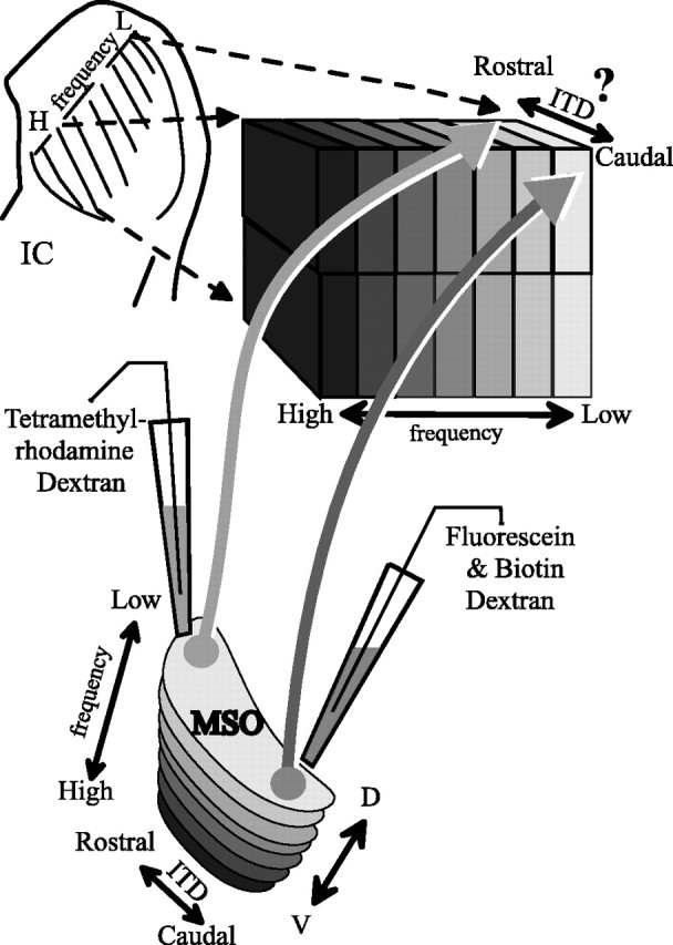
Experimental design and hypothesis. Interaural time differences (ITD) are hypothesized to be topographically organized along a rostrocaudal axis of the medial superior olive (MSO), within an isofrequency lamina. If so, the axons from MSO neurons are predicted to project to single laminas in the central nucleus of the inferior colliculus (IC) in a point-to-point manner. Injections of different labeled dextrans were made by iontophoresis in the same isofrequency plane to test this hypothesis. H, High frequency; L, low frequency; D, dorsal; V, ventral.

Materials and Methods

Surgery

There were two groups of experiments. In the first, anterograde tracers were injected into the right MSO, and in the second, retrograde tracers were injected into the right IC. Experiments were performed on 19 adult cats (Liberty Labs, Waverly, NY), and all procedures conformed to National Institutes of Health guidelines and protocols approved by the Animal Care Committee of the University of Connecticut Health Center. In all experiments, the animal was anesthetized with a mixture of ketamine (33 mg/kg) and xylazine (1 mg/kg), intubated, and then maintained in an areflexive state with a mixture of isoflurane and medical grade oxygen. It was monitored for breathing rate and reflexive state, maintained at 37°C with a water blanket, and received intravenous saline or lactated Ringer's solution during the procedure. The animal was placed in a double-walled sound attenuation chamber (IAC, Bronx, NY) and held in a stereotaxic device (Kopf, Tujunga, CA) for the MSO injections or in a custom head holder for the IC injections. For MSO injections, a craniotomy was performed over the cerebellum. For IC injections, a craniotomy was performed over the occipital cortex, and a small region of cortex was aspirated to permit visualization of the IC. After the recording and injections, the skin and muscles were sutured, the animal recovered in an intensive care unit incubator at 37°C until fully awake, and children's aspirin (40 mg) was administered immediately postoperatively as an analgesic. All animals recovered from surgery without permanent neurological impairment and were able to eat and drink normally.

Acoustic stimulation and recordings

In early experiments, acoustic stimuli were produced by a digital stimulus system (Rhode, 1976) under the control of an LSI-11/73 computer (Digital Equipment, Nashua, NH). In later experiments, acoustic stimuli were generated by a TDT System 2 (Tucker Davis Technologies, Gainesville, FL) under the control of a PC computer. All sounds were delivered by the same Beyer earphones (DT-48, Hicksville, NY) via sealed enclosures. The sound delivery system was calibrated from 60 to 40,000 Hz. For injections of anterograde tracers in MSO, sounds were delivered through the hollow ear bars of the stereotaxic device, and calibration was performed at the end of the ear bar with a 1/8 inch microphone (Brüel & Kjaer). For injections of retrograde tracers in IC, tones were delivered through a hollow tube in custom silicone ear molds (PER-FORM silicone ear impression material) made for each individual cat, similar to those used in the unanesthetized rabbit (Kuwada et al., 1987; Batra and Fitzpatrick, 1997). The hollow tube incorporated a probe that extended ∼2 mm beyond the end of the tube. Calibrations were performed through this probe using a 1/2 inch microphone (Brüel & Kjaer). These calibrations were then corrected for the characteristic of the probe.

The spectral and ITD sensitivities of neurons and multiunit clusters at the injection site were assessed in both the MSO and IC. Units were tested for their best frequency (BF) with monaural and binaural pure tones. Sensitivity of the units to ITD was measured with a binaural-beat stimulus (Kuwada et al., 1979; Batra et al., 1997a). Low-frequency units (BF ≤2500 Hz) and some with high BF were stimulated with pure tones in each ear that differed by 1 Hz. These stimuli produced a continuous change in the interaural phase difference. In one case, a low-frequency unit was tested with sinusoidally amplitude-modulated (SAM) tones with the same modulation frequency at both ears but with carrier frequencies that differed by 1 Hz. The sensitivity of high-frequency units (BF >2500 Hz) to ITDs was tested with a stimulus that consisted of SAM tones to either ear that had the same carrier frequency but modulation frequencies that differed by 1 Hz (Batra et al., 1997a). SAM tones were modulated to a depth of 80%. Test stimuli were 5100 msec in duration, but the first 100 msec was not analyzed. The best ITD based on a composite response was calculated (Yin and Kuwada, 1983; Kuwada et al., 1987; Batra et al., 1997a). The composite response was generated by averaging the responses at all frequencies that displayed significant synchrony to the 1 Hz beat frequency (Rayleigh test of uniformity; p < 0.001) (Mardia and Jupp, 1999).

Recordings were made with glass patch pipettes (2-20 μm tip, resistance 0.5-5 MΩ), and the same electrode was used for the injection. Electrodes were advanced with a microdrive (Burleigh Inchworm, Fishers, NY) mounted on the stereotaxic manipulator. For MSO injections, the electrode was initially positioned according to stereotaxic coordinates. An appropriate location for the IC or MSO injection was found by assessing neural responses to sound and making repeated penetrations. Acoustically driven responses of single or multiple units just above threshold were amplified with Dagan 2400 (Minneapolis, MN) and Princeton Applied Research (model 5113; Oak Ridge, TN) amplifiers. Action potentials were monitored by ear or discriminated by a BAK window discriminator and recorded with a unit event timer.

Injections

For injections of anterograde tracers in MSO, the electrodes were filled with one of two solutions of dextran in normal saline (Molecular Probes, Eugene, OR): (1) 10% tetramethyl-rhodamine (TMR) dextran (catalog #D-1817) or (2) a mixture containing 10% each of biotinylated dextran (BDA) (catalog #D-1956) and fluorescein-dextran (catalog #D-1820). Iontophoretic injections were made using a 51413 Precision Current Source (Stoelting, Wood Dale, IL) and currents of +2.0 to +3.5 μA(7sec pulses, 50% duty cycle, 5-23 min total duration). For injections of retrograde tracers in IC, several types of injection solutions were used, all mixed in normal saline: (1) 10% TMR dextran; (2) 6% Fluorogold (FG) (Fluorochrome, Inc., Denver, CO); (3) a mixture containing 3% FG and 5% BDA; (4) red latex microspheres (LumaFluor, Inc., Naples, FL) diluted 1:1; and (5) green latex microspheres (LumaFluor; 1:1). Microsphere injections required electrodes with 30-40 μm tips and pressure injections of 300-700 nl with a Picospritzer (General Valve, Fairfield, NJ).

Histology

After 7-10 d survival, animals were deeply anesthetized with the ketamine/xylazine mixture and killed by cardiac perfusion with 50 -75 ml of washout (2% sucrose and 0.05% lidocaine in 0.12 m phosphate buffer, pH 7.3-7.4) and 1000 ml of fixative (4% paraformaldehyde in 0.12 m phosphate buffer). Most brains with MSO injections (11 of 14) were cut in the frontal plane, and the remainder were cut in the horizontal plane perpendicular to it. Brains with IC injections were cut in the frontal plane (n = 4) or in the sagittal plane (n = 1). The tissue was cut on a freezing microtome into 50-μm-thick sections, collected in 0.12 m phosphate buffer, and stored at 4°C. In general, the histology for all experiments was designed to preserve the fluorescence of the different tracers or to convert the tracer into permanent nonfluorescent reaction products in alternate sections.

Fluorescent tracers

In cases with the MSO injections of dextran, every third section, beginning with the first, was mounted onto slides and coverslipped with 10% 1,4-diazabicyclo (2.2.2) octane (Sigma) in glycerine and neutral phosphate buffer. In most cases, sections were incubated first with Fluorescein Avidin DCS (A-2011; Vector Labs) at 1:1600. The fluorescein-labeled avidin binds with the BDA and adds to the signal emitted by the fluorescein-dextran. Fluorescent sections containing retrogradely transported red or green latex microspheres were dried onto subbed slides and coverslipped with Krystalon (64969/71; EM Science, Gibbstown, NJ) because the microspheres dissolve in glycerin-based mounting media.

Conversion of fluorescent tracers to permanent, nonfluorescent reaction products

Every third section from MSO injection cases was used.

Step 1. To render the biotinylated dextran visible, free-floating sections underwent avidin-biotin-HRP histochemistry (Oliver et al., 1994). After 20 min in 0.5% H₂0₂ in neutral phosphate buffer (0.12 m, pH 7.4) and rinses in buffered Triton X-100, sections were incubated in the ABC complex (PK-4000; Vector Labs) overnight at 4°C in the presence of 0.5 m NaCl. After rinses, sections were incubated in diaminobenzidine (DAB) (D-5637; Sigma) with Co and Ni for 15 min and then incubated in a fresh volume of the same DAB solution with 0.005% H₂0₂ for 15 min. In many experiments, additional sections received this same treatment (without step 2) and were used for Nissl stains.

Step 2. Next, the sections underwent an immunohistochemical reaction to render the TMR dextran permanently visible. After rinsing in neutral buffer, sections were blocked in neutral buffered 10% horse serum (Invitrogen; 16050-015) containing 0.1% Triton X-100 for 2 hr and then incubated in anti-tetramethylrhodamine antisera made in rabbit (A-6397; Molecular Probes), 1:12,000 dilution in the blocking solution and 0.15 m NaCl overnight at 4°C. After rinses in Triton X-100 buffer, sections were incubated with an anti-rabbit, biotinylated secondary antisera (Jackson 711-065-152), 1:800 dilution, for 4 hr at 25°C. After rinses in Triton X-100 buffer, the sections were exposed to the ABC complex (PK-4000; Vector) in the same buffer overnight at 4°C. Finally, the avidin-biotin-HRP complex was revealed with a DAB reaction without nickel or cobalt or, more often, a NovaRED reaction (SK-4800; Vector Labs), for 15 min. The sections were mounted from phosphate buffer onto subbed slides and cleared in Histoclear (HS-200; National Diagnostics) before coverslipping with Permount (SP15-500; Fisher). Earlier cases were treated with the freeze-thaw techniques to enhance immunostaining as outlined in Beckius et al. (1999), but this later proved to be unnecessary.

To render fluorescent FG permanently visible in a nonfluorescent form, an immunohistochemical method similar to that for anterograde transport of TMR dextran (step 2) was used on every third section in IC injection cases. After H₂0₂ treatment, buffer rinse, and blocking with horse serum, the sections were incubated in a primary anti-FG antisera made in rabbit (Chemicon AB153) 1:8000 overnight at 4°C. The same biotinylated anti-rabbit antisera followed by ABC reaction was used as in step 2 above. After the ABC reaction, a DAB incubation with nickel and cobalt was used, 4 min without H₂0₂ and 4 min with 0.0005% H₂0₂.

Analysis

Microscopic analysis used low-magnification camera lucida drawings and high-magnification analysis with computer-assisted microscope systems. Low-magnification, camera lucida drawings (20× magnification) were made with a Zeiss Axioskop microscope to show injection sites and dextran-filled axons. The axons and cell bodies labeled with fluorescent markers were viewed with epifluorescence microscopy [high numerical aperture (NA) ×10/NA 0.5 or ×25/NA 0.8 lenses], and microscopic data were collected with Neurolucida software (Microbrightfield, Colchester, VT) and an E-3200 Gateway computer. The microscopy system included a CCD video camera with gating capability for low-light conditions (CCD-72, Dage MTI, Michigan City, MI), a gating-integration controller (Instagator, model 105001, Dage MTI), a PC frame grabber-VGA card (FlashPoint Intrigue Lite, Integral Technologies, Indianapolis IN), a motorized stage controller (MC2000, Ludl Electronics Products, Hawthorne, NY), and a shutter for the mercury lamp (D122; UniBlitz, Vincent Associates, Rochester, NY). Data from nonfluorescent sections was collected with bright-field optics on the same microscope system. Analysis of the retrograde labeling in the MSO included three-dimensional (3D) reconstructions made with the Neurolucida system and displayed as solids (Solids Module, Microbrightfield, Inc.).

Axonal bouton densities in laminas of the IC were estimated to determine whether there were rostrocaudal gradients. In each case, we selected the most densely labeled lamina, and bouton counts in that lamina were made in serial nonfluorescent sections. For cases cut in the frontal or transverse plane (see Fig. 7A1), samples were obtained in regularly spaced sections (every third or sixth section). For the case cut in the horizontal plane (see Fig. 7B), every sixth horizontal section was sampled, and the lamina in each section was divided into seven regions along its rostrocaudal extent. Bouton counts within the individual samples were made with an optical fractionator (Stereo Investigator, Microbrightfield, Inc.). All of the boutons in the center half of the section thickness were counted within the sampled area. The number of boutons in a count was doubled to estimate the number of boutons in the entire section thickness. These complete reconstructions of all the boutons in the sample volume produced more reliable counts than single optical dissector planes within the section. This method conforms to stereological counting methods (Sterio, 1984; Coggeshall and Lekan, 1996) because all boutons within the sample volume were counted (a serial reconstruction), and the profiles at the edge were not counted twice.

Figure 7.

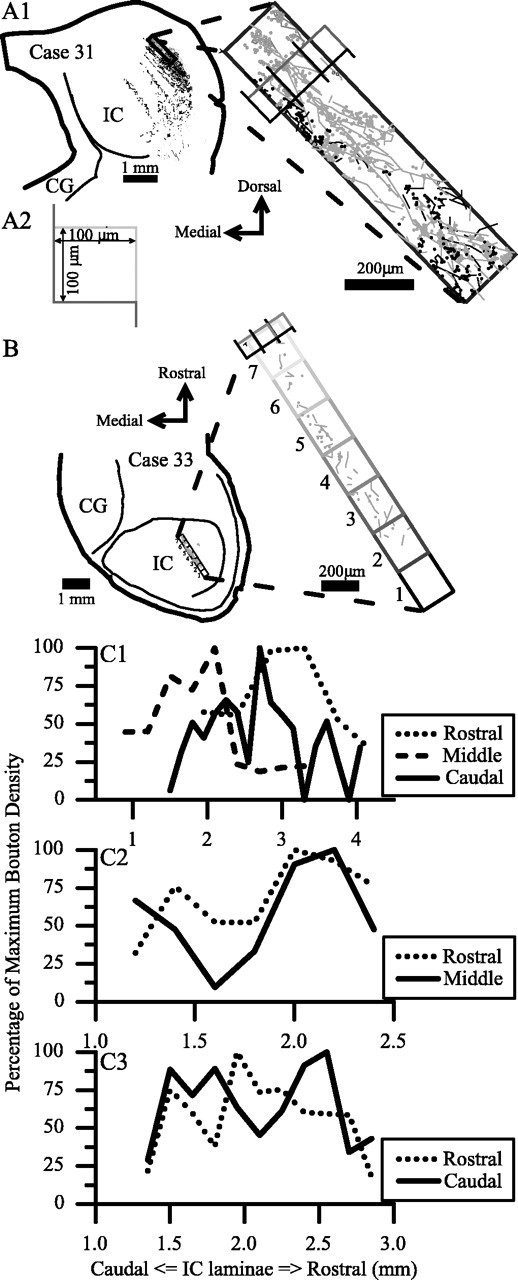
The density of boutons in single ICC laminas. A, In transverse sections (A1), bouton counts were made from within a single lamina, such as that shown in higher magnification to the right of the section. The two types of dextran-labeled axons in this case are shown in gray and black. The same lamina was identified and counted in each serial section. A counting frame (A2) was moved down the middle of the lamina to control the sampled area (the center of the rectangle in the higher magnification of the lamina). Boutons that intersected with the two gray edges of the counting frame were not included. B, Horizontal section showing the seven sample areas along the lamina in each section. These same sample areas were analyzed in each section and summed, and the sum corresponds to the bouton density from a single section in the transverse plane. C1, Histograms of bouton density in serial sections from three separate cases, each with its MSO injection in a different rostrocaudal location. The peaks of maximum bouton density are staggered in different sections along the rostrocaudal dimension of the IC. C2, Bouton density in serial sections after two injections in MSO at 1000 Hz BF at different rostrocaudal positions. Maximum bouton density is at the rostral end of the IC for both injections. C3, Bouton density in serial sections after two injections in MSO at 300 Hz BF at different rostrocaudal positions. Maximum bouton density from the rostral MSO is in the middle of the IC, whereas the caudal injection has peaks of high density rostrally and caudally in the IC.

The boutons plotted in the previous step were used to assess bouton gradients along the other axes perpendicular to the frequency axis (i.e., the dorsal-ventral axis and “oblique” axes between the dorsoventral and rostrocaudal axes). Three-dimensional serial reconstructions were made that allowed the sampled boutons to be viewed as a three-dimensional plane or contour, similar to the fibrodendritic lamina from which it was obtained. The three-dimensional field of boutons was projected onto two dimensions by rotating the contour until the planar surface was parallel to the viewing window (see Fig. 8C), and the differences in the Z coordinates were within the 200 μm thickness of the lamina. The X and Y coordinates of the markers at this orientation were then rendered as a two-dimensional scatter plot (see Fig. 8 D). To examine the density of boutons in the plane of the lamina, perpendicular to the frequency axis, we rotated the field of bouton markers in 10° increments. A histogram of bouton density perpendicular to the x-axis with 150 -200 μm bins was generated at each angle of rotation.

Figure 8.

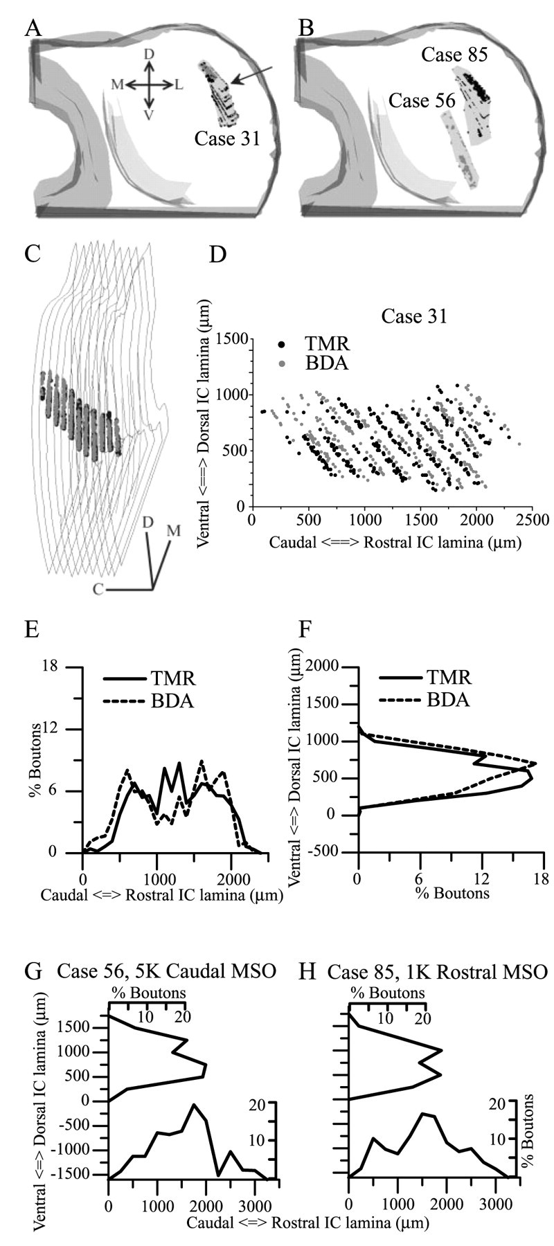
Measurements of bouton gradients along arbitrary axes perpendicular to the frequency axis. A, Three-dimensional reconstruction of sampled boutons in case 31 (BF 300 Hz). The sampled area in each section is enclosed in a rectangle. B, Reconstructions of sampled boutons in case 85 (BF 1 kHz) and case 56 (BF 5 kHz). C, Case 31 after rotation so that the surface of the lamina enclosing the boutons is parallel to the plane of view. The viewing angle is indicated by the arrow in A. D, The boutons in C have been flattened onto the x-y plane and rotated so that the longest axis is parallel to the x-axis of the graph. Only 300 TMR (black) and BDA (gray) randomly selected boutons terminals are shown, and the BDA bouton terminals have been offset from the TMR terminals by 3% to the right for the purpose of illustration. All bouton terminals were included in the analyses shown in E-H. E, The number of boutons, as a percentage of all the boutons of the same type, are plotted as a function of x-axis position (E, parallel to the long axis) and y-axis position (F, perpendicular to the long axis). The same bin width is used in both histograms. The distribution of boutons along other axes was also checked by rotating the data in 10° steps and replotting the histograms (data not shown). G, Bouton distribution in case 56, parallel to the longest axis (plotted along the x-axis) and perpendicular to that plotted along the y-axis. H, Bouton distribution in case 85. C, Caudal; D, dorsal; M, medial; L, lateral; V, ventral.

Results

Injections of dextran into MSO

Because the goal of the study was to examine the topography of the projection from the MSO to the IC (Fig. 1), we made small injections of dextran into the MSO that resulted in axonal transport to the IC. The injections were confined to the MSO or extended beyond the margins of the MSO, but they did not invade the lateral superior olive (LSO). Figure 2 shows an injection of BDA mixed with fluorescein-dextran in the caudal MSO (Fig. 2A) and an injection of TMR dextran in the same MSO at the rostral end (Fig. 2B). A single injection from another case is shown in Figure 2C, and its location at the dorsal aspect of MSO can be discerned from the cytoarchitecture of the superior olive in the adjacent Nissl-stained section (Fig. 2D).

Figure 2.

Injections of dextran in MSO seen in transverse sections after conversion to nonfluorescent reaction product. A, An injection of BDA in the caudal MSO in case 31 at a BF of 300 Hz. B, An injection of TMR dextran in rostral MSO in the same case as A. C, An injection of BDA in dorsal MSO in case 55. D, A Nissl-stained section adjacent to that in C showing the cytoarchitecture of MSO. LSO, Lateral superior olivary nucleus. Scale bar, 200 μm.

We identified the rostrocaudal position in the MSO of each injection site and its BF. Most of the injection sites were in the rostral half of the MSO. The locations of all injections are shown in Figure 3A, which depicts the MSO as a flat sheet, with low frequency at the top (dorsal in vivo) and high frequency at the bottom of the y-axis (ventral in vivo), whereas the rostrocaudal dimension of the MSO is the x-axis. The center of each injection site is marked by a symbol, and its rostrocaudal extent is indicated by the length of the corresponding bar. The horizontal line on which each bar lies indicates the length of the MSO in that animal. The BF at each injection site is represented by the vertical position of the symbols. The BFs covered a broad range: 200 Hz to 9 kHz. In two animals, two injections were made in the same MSO, and both injection sites had similar best frequencies (300 Hz in case 31 and 1 kHz in case 33). Eight injections were made at low frequencies (<2500 Hz). Of these, four were made at a BF of ∼1 kHz. Four single injections were made at higher frequency. In one animal, the injection site was very ventral and caudal in MSO, and recordings were made at this site from two separate units with BFs of 5.3 and 9.2 kHz (Fig. 3A) (plotted at 5 kHz).

Figure 3.

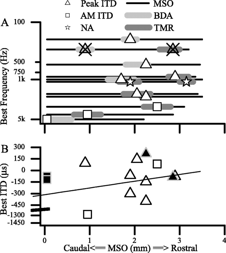
Locations and physiological characteristics of injection sites in MSO. A, Best frequencies and rostrocaudal locations of injection sites in MSO. In some cases (triangles with X, stars), two injections matched in frequency were made in the same MSO at two different rostrocaudal locations. Note that recordings of best ITD were not available (NA, stars) at all injection sites. B, Relationship of best ITD at injection site to the rostrocaudal position in MSO. Positive ITDs indicate contralateral delays and correspond to sounds emanating from the ipsilateral hemifield. Lines fit to all data are similar to that of Yin and Chan (1990) with units near zero ITD tending to be more rostral. Closed symbols denote single-unit recordings; open symbols are multiunit recordings.

There was no clear relationship between the best ITD and the rostrocaudal location of the injection sites in the MSO. Figure 3B shows the location of all injection sites along the rostrocaudal axis of the MSO relative to the best ITD recorded at that site. (High-frequency units that were sensitive to ITDs in envelopes are shown as squares.) The units at the injection sites were excited by inputs to either ear and generally exhibited ITD sensitivity similar to that seen in previous studies of the anesthetized cat (Yin and Chan, 1990). Units had predominantly “peak-type” responses in that they discharged maximally at the same ITD at all frequencies with which they were tested. Most units in our sample were tuned to ITDs within the free-field range of the cat (approximately ±325 μsec) (Roth et al., 1980), and most characteristic delays (7 of 10) and best ITDs (11 of 12) were within this range. Nevertheless, individual units recorded at different locations in the same MSO could show responses at variance with the rough rostrocaudal gradient of best ITD demonstrated by Yin and Chan (1990) (Fig. 3B, regression line). Recordings at BF 300 Hz (Figs. 2A,B, 3A, triangles with X) are shown in Figure 4. Here, the best ITD at the rostral site (Fig. 4, top) was -86 μsec, whereas at the more caudal site it was 94 μsec. As in the previous study, the best ITD of the recording did not predict its location in the MSO.

Figure 4.

Neuronal recordings in the same MSO (case 31, BF 300 Hz) could be tuned to ITDs running counter to the postulated ITD topography. A, Rostral MSO single-unit recording (3 mm anterior to the caudal end of MSO). B, Caudal MSO multiunit recording (1 mm from caudal end of MSO). Left panels, Response as a function of ITD at different frequencies constructed from responses to binaural-beat stimuli. Right panels, Composite delay curves calculated by averaging the responses shown in the left panel. The best ITD is the peak of the curve. TMR, Tetramethylrhodamine dextran; BDA, biotinylated dextran amine.

Termination pattern of MSO axons in IC

Axons that terminated in IC were distinguished by the presence of terminal boutons (Fig. 5C, micrographs 176 and inset 171′), that is, the swelling at the Node of Ranvier or end of the axonal branch that indicates presynaptic specializations and the location of synaptic contacts (Oliver et al., 1995). Only axons with boutons are considered in this analysis. After the two injections in the same MSO in case 31, the axons from each injection were labeled with a different color and could be easily distinguished within the same section. In fluorescent sections, axons labeled with TMR were red, whereas axons labeled with the BDA-fluorescein dextran mixture were green (Fig. 5C, micrograph 176). In nonfluorescent sections processed for immunocytochemistry, boutons labeled with TMR were red, and those labeled with BDA were black (Fig. 5C, micrograph inset 171′).

Figure 5.

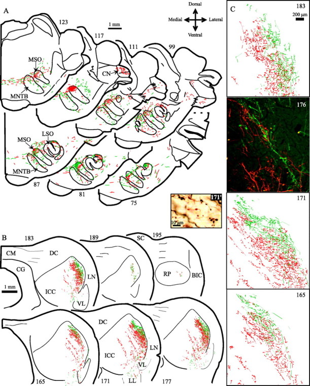
MSO injections and laminar IC projections in case 31. A, Transverse sections to show MSO injections at 300 Hz BF at two different rostrocaudal positions. BDA injection (green, caudal); TMR dextran injection (red, rostral). Higher numbered sections are at more rostral levels. B, Transverse sections that show axons from MSO injections projecting to central nucleus of IC (ICC). Axons from the rostral injection (red) overlap those from the caudal injection (green), and both types are found throughout the rostrocaudal extent of the central nucleus. C, Higher magnification plots and micrographs show the boutons of axons labeled with the two tracers. Bouton fields partially overlap. Boutons with the two colors are easily distinguished in digital micrographs of the axons with fluorescent labeling and after conversion of the dextran to nonfluorescent form. In section 176, two digital, monochrome images of the same field were taken with rhodamine and fluorescein filter sets and a ×10/NA 0.5 lens, and then combined to make a red-green-blue image. In section 171′, boutons are imaged with a color digital camera and ×40/NA 1.3 lens. All images were adjusted for color level, contrast, and brightness. BIC, Brachium of IC; CG, central gray; CM, commissure of IC; CN, cochlear nucleus; DC, dorsal cortex; LL, lateral lemniscus; MNTB, medial nucleus of the trapezoid body; RP, rostral pole nucleus; SC, superior colliculus; VL, ventrolateral nucleus.

Axons from a single point in MSO terminated along the entire rostrocaudal extent of the laminas in the ICC. These terminal fields were continuous in the rostrocaudal direction throughout the central nucleus (Fig. 5B, ICC) and stopped dorsally ∼0.5 mm short of the border with the dorsal cortex (Fig. 5B, DC). Small numbers of collaterals extended into the rostral pole nucleus (Fig. 5B, section 195, RP) at the level of the superior colliculus.

Inputs from two points in the MSO to the ICC overlapped along the rostrocaudal dimension. In the case depicted in Figure 5, two small injections (Figs. 2A,B,5A, sections 81 and 117) were made in the same MSO at the same BF (300 Hz). TMR-labeled axons (red) from the rostral injection (Fig. 5A, section 117) overlapped fluorescein-dextran-labeled axons (green) from the caudal injection (Fig. 5A, section 81) in the dorsolateral corner of the central nucleus (Fig. 5B). The zone of overlap was at least 200 μm wide and was seen in all sections through the central nucleus (Fig. 5C).

The labeling in the ICC from the two injections differed slightly in that the TMR axons were located somewhat more ventromedially (Fig. 5C, red axons, sections 165-183). Although the most lateral of this labeling was continuous rostrocaudally, separate bands of label were seen medially. The most medial labeling consisted of narrow, 200 μm bands of labeled axons separated by wider gaps. In contrast, the BDA-labeled axons from the caudal injection (Fig. 5A, section 81) were more dorsolateral in the central nucleus. The slight offset in the labeling may have been a result of spread of the tracer in MSO to sections coding somewhat different frequencies, although both injections were centered at the same BF.

Another example of how a single point in MSO sends axons along the entire rostrocaudal length of the ICC is shown in Figure 6. This case also compares the results of two injections made at different rostrocaudal positions in the same MSO (Fig. 6A). Most axons terminated in a single lamina that can be seen by reconstructing the entire IC in 3D and rotating the reconstruction 40° (Fig. 6B). Because the sections in this case were cut in the horizontal plane (section 225, inset), the distribution of the axons along the laminas is seen as labeling from caudolateral to rostromedial (Fig. 6C, sections 219 -237) (the dorsal-most sections have the highest numbers). Each panel shows the MSO projections in three adjacent sections that were processed with different histological methods. In each section, terminals from both injections contribute to labeling along the length of the lamina except in the dorsal-most section, where blood vessels interrupt the lamina.

Figure 6.

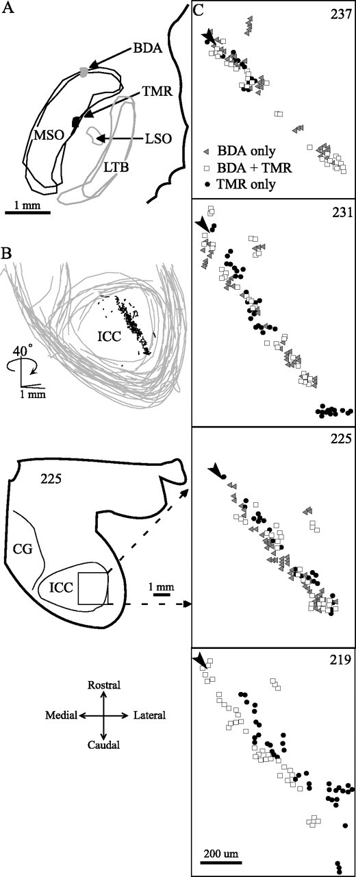
MSO axons converge on a single ICC lamina in case 33. A, Injections in MSO at two recording sites with 1000 Hz BF. B, Serial 3D reconstruction made from individual plots of sections through the IC. The 40° rotation around the y-axis shows the lamina in which the axons terminate at its narrowest, on-edge view. Almost all of the labeling is confined to this one lamina. C, Higher-magnification plots to show the projections in the IC labeled from both MSO injection sites. Arrowheads indicate the rostromedial end of the lamina. Each drawing shows the combined labeling from three adjacent horizontal sections (no rotation) prepared with different histological methods to reveal BDA, TMR, or BDA + TMR. Because of a technical problem, the distinction of TMR from BDA in one section was not definitive. This section designated “BDA + TMR” does not imply that the same axons were labeled by both tracers. LTB, Lateral trapezoid body.

Distribution of synaptic boutons from MSO axons in ICC laminas

Point-to-point connections between MSO and IC isofrequency laminas appear to be absent on the basis of results of the small MSO injections presented above. If there is a gradient in the representation of ITD in the MSO perpendicular to the frequency axis, however, it could be transmitted to the IC effectively by a gradient in the density of the synapses, even if there are no point-to-point connections. If such a gradient were present in the rostrocaudal direction, for example, neurons in the caudal MSO might make a higher density of synaptic contacts in the caudal part of the isofrequency laminas in ICC, whereas rostral MSO neurons might terminate more densely in the rostral IC. To examine this possibility, axonal boutons were counted in a single lamina in the ICC of five animals (Fig. 7). Electron microscopy shows that boutons are the sites of synaptic contacts made by axons from MSO (Oliver et al., 1995). The boutons can be identified clearly and analyzed at the light microscopic level (Fig. 5C, sections 176, 171′). It was relatively easy to identify the same lamina in sections cut in the transverse plane (Fig. 7A1) or horizontal plane (Fig. 7B), and we could compare the density of boutons in each sample. Boutons were counted in the central 100 μm of the 200-μm-thick lamina (Fig. 7A1, inset, A2).

The first analysis was bouton density measured in serial sections through the IC (Fig. 7C1-C3). Boutons were not distributed in a consistent way. Because boutons were counted from the caudal-most section of the IC, none of the samples revealed a systematic increase or decrease in the bouton density that covaried with the rostrocaudal position of the injection in the MSO (Fig. 7C1). However, different points along a lamina received different amounts of input. In the three cases shown in Figure 7C1, the maximum bouton density was located near the middle of each of the ICC laminas, but the peaks are staggered along the x-axis. Because these cases differed in the rostrocaudal length of the IC lamina and the BF, this appearance may be a byproduct of laminas that began at different positions relative to the caudal-most section through the IC. More informative were the two cases in which two injections were made at the same BF at different rostrocaudal positions in the MSO (Figs. 5, 6). Case 33 (Fig. 7C2) showed a maximum bouton density at the rostral end of the ICC laminas for both injections. Case 31 (Fig. 7C3) had the maximum density from rostral MSO in the middle of the IC lamina, whereas the caudal injection had peaks of high density rostrally and caudally in the ICC.

The second analysis of bouton density was made after a three-dimensional reconstruction of the lamina from which the boutons were counted. Three cases cut in the transverse plane are shown for comparison. In one case the BF was 300 Hz (Fig. 8A), and in the other two cases the BFs were 1 and 5 kHz (Fig. 8B) (cases 85 and 56, respectively). The boutons in a single lamina were rotated to essentially a two-dimensional surface in the plane of the page (Fig. 8C). In this way, the density of the boutons could be observed along all possible axes perpendicular to the frequency axis, i.e., the axis orthogonal to the two-dimensional surface (Fig. 8D). In two-dimensional scatter plots of the boutons, it was evident that the two inputs labeled in the same case were generally coextensive in the lamina (Fig. 8D, black and gray spheres), and there was not a systematic separation of inputs as has been seen in the projections of lateral superior olive and dorsal cochlear nucleus to the same lamina (Oliver et al., 1997); however, the density of the inputs was not homogeneous, and there were patches of several hundred micrometers in diameter in which one input was more prevalent than the other. There was little evidence for a linear gradient of bouton density in any direction. When histograms of bouton density were made at different angles of orientation, the density of boutons varied most dramatically when it was measured parallel to the longest axis of the laminar plane (Fig. 8E), similarly equivalent to measurements made for the sectional analysis (Fig. 7), and least dramatically when perpendicular to the longest axis (Fig. 8F). Other axes were similar to one of these two extremes. The density of termination along most axes showed one or more prominent peaks, but these were not related to the location of the MSO injection (Fig. 8E,G,H).

What is clear from both the sectional and three-dimensional analysis is the lack of a uniform bouton density or linear gradient along any dimension of the ICC laminas. Moreover, the proportion of synaptic inputs from different parts of MSO, as represented by boutons, varies almost randomly along a lamina and in a way that was not systematically related to the location of the injection within MSO.

Injections in IC and retrograde labeling of MSO neurons

The experiments above revealed little evidence for transmission of a point-to-point map of azimuth from MSO to IC and suggested a divergence of projections from MSO neurons. Some MSO neurons with axons projecting to an entire IC lamina might be intermingled with neurons with axons that have more restricted projections. In the case of this “mixed divergence,” we would predict that a focal injection of retrograde tracer in the IC might produce denser labeling in some parts of the MSO than in others, and this pattern might vary with the rostrocaudal position of the injection site. On the other hand, if all axons diverged completely, we would expect a uniform distribution of retrogradely labeled cells, and this pattern would not vary dramatically with the rostrocaudal position of the IC injection.

The data from retrograde transport is consistent with MSO neurons that have completely divergent projections. In all cases, labeled neurons were distributed evenly along the rostrocaudal extent of MSO, regardless of the location of the injection site in the IC. Injections of retrograde tracers were made in the low-frequency IC and were relatively restricted in their rostrocaudal spread along the laminas of the central nucleus (Fig. 9). Two injections were in the mid ICC at frequencies <400 Hz (Fig. 9A,B, gray, IC/Horizontal View), and the caudal part of the injection site was at the same level as the caudal-most commissure of the IC. A third injection (Fig. 9C, gray, IC/Horizontal View) was in the rostral ICC at a similar BF (350 Hz). All three injections produced a similar pattern of labeling in MSO (Fig. 9A-C, gray spheres in MSO/Lateral View) with labeled neurons at the dorsal edge of MSO at all rostrocaudal levels. Injections at the same BF in the dorsal cortex of IC rostrally (Fig. 9A, DC, black, in IC/Horizontal View) or caudal cortex (Fig. 9B, CC, black, in IC/Horizontal View) produced either no or few labeled cells (Fig. 9B, black spheres in MSO), respectively, at the same locations. In contrast, an injection at 1000 Hz in rostral central nucleus (Fig. 9C, black, IC/Horizontal View) resulted in a continuous band of labeled cells just below the labeled cells from the lower-frequency site (Fig. 9C, black spheres in MSO).

Figure 9.

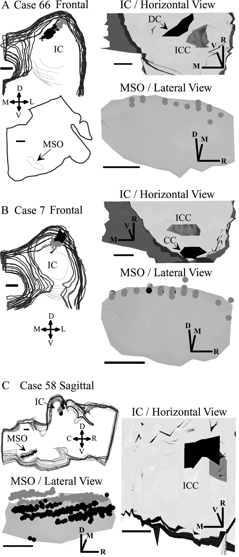
Retrograde labeling in MSO after injections in IC. A, Injections of green (gray) and red (black) latex microspheres in IC of case 66 and retrograde transport to MSO. Stacks of frontal (transverse) sections show the IC injection (left). A single section from the brainstem at the level of the superior olive shows MSO (arrow). The 3D solids reconstruction of the injection sites in the IC shows a horizontal view as seen from the dorsal surface of the brain (top right). The IC is transparent so that the locations of the injection sites can be seen. The 3D solids reconstruction of MSO shows retrogradely labeled neurons (bottom right, gray spheres). The MSO in the lateral view is rotated 45° around the rostrocaudal axis so that it appears as a flat surface parallel to the page. This view of MSO is as if the eye were at the location indicated by the arrow. B, Injections of green (gray) and red (black) microspheres in frontal sections of case 7 and retrogradely labeled neurons in MSO (gray and black spheres, respectively) (details are in A). C, Injections of fluorogold (gray) at 350 Hz BF and redlatex microspheres (black) at 1k Hz BF. Stacks of sagittal sections are at top left. Horizontal view of IC (right) and lateral view of MSO (left bottom) show retrogradely labeled neurons in MSO (gray and black spheres) as in A and B. D, Dorsal; R, rostral; L, lateral; M, medial; V, ventral. Scale bars, 1 mm.

The density of the labeled neurons along the rostrocaudal axis of MSO was not obviously related to the location of the injection site. Although the two cases at mid IC had nearly the same location, these small injections produced small numbers of labeled cells in each section and with slightly fewer labeled cells at the rostral end in one case and the caudal end in the other case (Fig. 9A,B). The somewhat larger injection in the rostral IC (Fig. 9C, black) produced a denser but nearly continuous band of labeled neurons. The most obvious discontinuities in Figure 9C are related to the 3D reconstructions from sagittal sections and not the location of the injection site.

Discussion

The present results imply that a simple, linear system of fine-grain, point-to-point connections does not convey a spatial map of ITD, or any other stimulus parameter, from the MSO to the IC. Small groups of adjacent neurons labeled with anterograde tracers send their axons along the entire length of laminas in the central nucleus of the IC. Quantitative analysis of the boutons from these axons shows that the synapses from these axons do not exhibit a gradient in density related to their connections to the MSO. The arrangement of retrogradely labeled neurons in MSO also supports the absence of a gradient because points in the IC laminas receive convergent inputs from neurons that are evenly distributed along the rostrocaudal extent of the MSO. These data suggest that information about the azimuthal location of a sound source in the IC does not depend on a simple map transmitted from the MSO.

Topography of ITD coding in MSO

Our data provide no support for the idea that the azimuth is encoded by MSO neurons arranged rostrocaudally according to the best ITD, but they do not rule out this possibility. Indeed, the recordings at injection sites indicate that any topography that is present for ITD must be weak. Yin and Chan (1990) provided evidence for such a topography by merging data from several animals. Although our sample of recordings from low-frequency MSO neurons was weighted toward the rostral half, the two widely separated recordings in the same MSO had best ITDs inconsistent with the assumed topographical arrangement. Both the individual and paired recordings suggest a large degree of variability even within the same animal. In our study, some of the variability may have been caused by our use of multiunit recordings, but similar variability is present in the data of Yin and Chan (1990). Some neurons at a single rostrocaudal position had very different best ITDs, and neurons with similar best ITDs were found at very different rostrocaudal locations (Yin and Chan, 1990, their Fig. 13). Thus, any map of ITD in the MSO must be coarse, at best.

Coarse mapping of ITD in IC?

The present data suggest that the individual MSO axons terminate along the entire rostrocaudal length of the fibrodendritic laminas in the central nucleus of the IC rather than in discrete point-to-point connections. It is unlikely that this rostrocaudally extensive projection to the ICC is caused by the diffusion of tracer along the rostrocaudal axis of MSO because the present injections were restricted in their rostrocaudal spread. Moreover, our results are unlikely to be caused by fibers of passage in the injection sites. Although we cannot absolutely rule out fibers of passage, their contribution seems minimal. If fibers of passage were a problem, they should be seen in the two cases with two injections in MSO. We would expect the rostral injections to produce more labeling in the IC than the caudal injections because MSO efferents run parallel to the nucleus to exit rostrally. Plus, axons with both fluorescent labels should be observed but were not. A final argument that minimizes the contribution of fibers of passage is that the results of the anterograde experiments are fully consistent with the findings from retrograde experiments.

Topographical maps relevant to ITD processing were not a focus of previous anatomical studies of MSO projections to the IC. Early studies with lesion methods (Van Noort, 1969) and retrograde methods (Roth et al., 1978; Adams, 1979; Brunso-Bechtold et al., 1981; Aitkin and Schuck, 1985; Maffi and Aitkin, 1987) emphasized the laterality of the projections and the convergence of inputs from different sources. The tonotopic organization of these midbrain projections was described in the cat and in nucleus laminaris of the barn owl in studies using autoradiographic tracing methods (Henkel and Spangler, 1983; Takahashi and Konishi, 1988). In these studies, there was extensive rostrocaudal labeling in IC; however, those studies could not distinguish labeled axons from labeled synaptic boutons, and the size of the injections relative to the size of the MSO or nucleus laminaris was larger than in the present studies.

Despite rostrocaudally projecting axons along an isofrequency lamina, could these axons convey a coarse map of ITD? One method to convey a coarse map from different MSO sites would be a coarse shift in the entire projection to the ICC that varies systematically from one site to another. Shifts in labeling were not reported in previous studies of the cat (reference citations above), but those studies did not specifically look for such a shift; however, a rostrocaudal shift in the projections to IC was reported in the barn owl (Takahashi and Konishi, 1988). Injections at different positions along the ITD axis were made in nucleus laminaris in different owls. In the present data, reproducible shifts in the boutons were not found in any dimensions of the ICC perpendicular to the frequency axis; however, a coarse map of ITD could be conveyed by an uneven distribution of synaptic inputs along a lamina. Our findings suggest that MSO axons may distribute their synaptic inputs heterogeneously as they travel along the ICC lamina.

The encoding of ITD in the IC

Our results make it unlikely that any map of ITD in the MSO is transmitted by point-to-point topography to the IC. Thus, if there is a topographical organization of stimulus azimuth in the IC, as suggested by free-field recordings (Aitkin et al., 1985), it is not a reflection of a spatially mapped projection from the MSO. The question therefore arises: how is ITD encoded in the IC? Two broad systems are possible.

The first is that the IC encodes only an average ITD, signaling a sound in the contralateral hemifield (McAlpine et al., 2001). The true ITD is decoded at a higher level by weighing the relative activities of neurons in the left and right IC. In this view, the pattern of innervation in IC reflects the averaging of ITD information from the MSO of one side. Such averaging would not completely obliterate sensitivity to ITD, because most neurons in the MSO are tuned to ITDs corresponding to sounds in the contralateral hemifield; however, such a system would predict tuning in the IC that is broader than that in the MSO. Exactly the opposite has been reported: tuning to ITDs appears to be sharper in the IC than in the MSO (Yin and Chan, 1990; Fitzpatrick et al., 1997). Thus, the system appears to require encoding of ITDs on a relatively fine scale.

An alternative possibility is that ITD could be encoded by groups of neurons sensitive to particular ITDs, but these neurons may be organized in a nonlinear map. Neurons with different best ITDs may be located in different regions within a lamina in the ICC. Our finding that the MSO boutons are distributed with an uneven density within a single lamina suggests that an ICC neuron at one point in the lamina may receive a heavier input from one point in MSO than from another. This would create ICC neurons with different ITDs distributed almost randomly within a lamina.

ITD-sensitive inputs from other sources might converge with MSO inputs to contribute to an irregular spatial distribution of ITD sensitivity in ICC. Both anatomical (Oliver, 2000) and physiological (Stanford et al., 1992; Batra et al., 1993; McAlpine et al., 1998) data support convergence in the IC. Neurons sensitive to ITDs are present in the LSO (Finlayson and Caspary, 1991; Joris and Yin, 1995; Batra et al., 1997a,b) and in the dorsal nucleus of the lateral lemniscus (DNLL) (Brugge et al., 1970), and both of these nuclei project to the IC where they may converge with the inputs from the MSO. Because the ipsilateral LSO and DNLL provide inhibition to the IC and may terminate on separate parts of a lamina (Oliver, 2000), the particular pattern of convergence may produce zones with different functionality and a nonlinear, distributed arrangement of ITD sensitivity.

Cellular mechanisms are also likely to shape the network that codes sound location in the IC. There is a heterogeneous population of neurons in the IC (Peruzzi et al., 2000; Sivaramakrishnan and Oliver, 2001), some of which may receive more MSO inputs than others. Local interconnections within the IC (Oliver and Morest, 1984; Oliver et al., 1991) may be important to combine ITD, interaural level, and spectral information. Most exciting is the recent discovery that IC neurons show long-term potentiation (Wu et al., 2002) and plasticity (Ma and Suga, 2001). This suggests that local synaptic mechanisms may be involved in coding sound location in the ICC.

References

- Adams JC ( 1979) Ascending projections to the inferior colliculus. J Comp Neurol 183: 519-538. [DOI] [PubMed] [Google Scholar]
- Aitkin L, Schuck D ( 1985) Low frequency neurons in the lateral central nucleus of the cat inferior colliculus receive their input predominantly from the medial superior olive. Hear Res 17: 87-93. [DOI] [PubMed] [Google Scholar]
- Aitkin LM, Pettigrew JD, Calford MB, Phillips SC, Wise LZ ( 1985) Representation of stimulus azimuth by low-frequency neurons in inferior colliculus of the cat. J Neurophysiol 53: 43-59. [DOI] [PubMed] [Google Scholar]
- Batra R, Fitzpatrick DC ( 1997) Neurons sensitive to interaural temporal disparities in the medial part of the ventral nucleus of the lateral lemniscus. J Neurophysiol 78: 511-515. [DOI] [PubMed] [Google Scholar]
- Batra R, Kuwada S, Stanford TR ( 1993) High-frequency neurons in the inferior colliculus that are sensitive to interaural delays of amplitude-modulated tones: evidence for dual binaural influences. J Neurophysiol 70: 64-80. [DOI] [PubMed] [Google Scholar]
- Batra R, Kuwada S, Fitzpatrick DC ( 1997a) Sensitivity to interaural temporal disparities of low- and high-frequency neurons in the superior olivary complex: I. Heterogeneity of responses. J Neurophysiol 78: 1222-1236. [DOI] [PubMed] [Google Scholar]
- Batra R, Kuwada S, Fitzpatrick DC ( 1997b) Sensitivity to interaural temporal disparities of low- and high-frequency neurons in the superior olivary complex: II. Coincidence detection. J Neurophysiol 78: 1237-1247. [DOI] [PubMed] [Google Scholar]
- Beckius GE, Batra R, Oliver DL ( 1999) Axons from anteroventral cochlear nucleus that terminate in medial superior olive of cat: observations related to delay lines. J Neurosci 19: 3146-3161. [DOI] [PMC free article] [PubMed] [Google Scholar]
- Brand A, Behrend O, Marquardt T, McAlpine D, Grothe B ( 2002) Precise inhibition is essential for microsecond interaural time difference coding. Nature 417: 543-547. [DOI] [PubMed] [Google Scholar]
- Brugge JF, Anderson DJ, Aitkin LM ( 1970) Responses of neurons in the dorsal nucleus of the lateral lemniscus of cat to binaural tonal stimulation. J Neurophysiol 33: 441-458. [DOI] [PubMed] [Google Scholar]
- Brunso-Bechtold JK, Thompson GC, Masterton RB ( 1981) HRP study of the organization of auditory afferents ascending to central nucleus of inferior colliculus in cat. J Comp Neurol 197: 705-722. [DOI] [PubMed] [Google Scholar]
- Carr CE, Konishi M ( 1988) Axonal delay lines for time measurement in the owl's brainstem. Proc Natl Acad Sci USA 85: 8311-8315. [DOI] [PMC free article] [PubMed] [Google Scholar]
- Coggeshall RE, Lekan HA ( 1996) Methods for determining numbers of cells and synapses: a case for more uniform standards of review. J Comp Neurol 364: 6-15. [DOI] [PubMed] [Google Scholar]
- Cook DL, Schwindt PC, Grande LA, Spain WJ ( 2003) Synaptic depression in the localization of sound. Nature 421: 66-70. [DOI] [PubMed] [Google Scholar]
- Finlayson PG, Caspary DM ( 1991) Low-frequency neurons in the lateral superior olive exhibit phase-sensitive binaural inhibition. J Neurophysiol 65: 598-605. [DOI] [PubMed] [Google Scholar]
- Fitzpatrick DC, Batra R, Stanford TR, Kuwada S ( 1997) A neuronal population code for sound localization. Nature 388: 871-874. [DOI] [PubMed] [Google Scholar]
- Goldberg JM, Brown PB ( 1969) Response properties of binaural neurons of dog superior olivary complex to dichotic tonal stimuli: some physiological mechanisms of sound localization. J Neurophysiol 32: 613-636. [DOI] [PubMed] [Google Scholar]
- Hafter ER, Trahiotis C ( 1997) Functions of the binaural system. In: Encyclopedia of acoustics (Crocker MJ, ed), pp 1461-1480. New York: Wiley.
- Henkel CK, Spangler KM ( 1983) Organization of the efferent projections of the medial superior olivary nucleus in the cat as revealed by HRP and autoradiographic tracing methods. J Comp Neurol 221: 416-428. [DOI] [PubMed] [Google Scholar]
- Irvine DR, Gago G ( 1990) Binaural interaction in high-frequency neurons in inferior colliculus of the cat: effects of variations in sound pressure level on sensitivity to interaural intensity differences. J Neurophysiol 63: 570-591. [DOI] [PubMed] [Google Scholar]
- Joris PX, Yin TCT ( 1995) Envelope coding in the lateral superior olive. I. Sensitivity to interaural time differences. J Neurophysiol 73: 1043-1062. [DOI] [PubMed] [Google Scholar]
- Kuwada S, Yin TCT, Wickesberg RE ( 1979) Response of cat inferior colliculus neurons to binaural beat stimuli: possible mechanisms for sound localization. Science 206: 586-588. [DOI] [PubMed] [Google Scholar]
- Kuwada S, Stanford TR, Batra R ( 1987) Interaural phase-sensitive units in the inferior colliculus of the unanesthetized rabbit: effects of changing phase. J Neurophysiol 57: 1338-1360. [DOI] [PubMed] [Google Scholar]
- Ma X, Suga N ( 2001) Plasticity of bat's central auditory system evoked by focal electric stimulation of auditory and/or somatosensory cortices. J Neurophysiol 85: 1078-1087. [DOI] [PubMed] [Google Scholar]
- Maffi CL, Aitkin LM ( 1987) Differential neural projections to regions of the inferior colliculus of the cat responsive to high frequency sounds. Hear Res 26: 211-219. [DOI] [PubMed] [Google Scholar]
- Mardia KV, Jupp PE ( 1999) Directional statistics. New York: Wiley.
- McAlpine D, Jiang D, Shackleton TM, Palmer AR ( 1998) Convergent input from brainstem coincidence detectors onto delay-sensitive neurons in the inferior colliculus. J Neurosci 18: 6026-6039. [DOI] [PMC free article] [PubMed] [Google Scholar]
- McAlpine D, Jiang D, Palmer AR ( 2001) A neural code for low-frequency sound localization in mammals. Nat Neurosci 4: 396-401. [DOI] [PubMed] [Google Scholar]
- Oliver DL ( 2000) Ascending efferent projections of the superior olivary complex. Microsc Res Tech 51: 355-363. [DOI] [PubMed] [Google Scholar]
- Oliver DL, Morest DK ( 1984) The central nucleus of the inferior colliculus in the cat. J Comp Neurol 222: 237-264. [DOI] [PubMed] [Google Scholar]
- Oliver DL, Kuwada S, Yin TC, Haberly LB, Henkel CK ( 1991) Dendritic and axonal morphology of HRP-injected neurons in the inferior colliculus of the cat. J Comp Neurol 303: 75-100. [DOI] [PubMed] [Google Scholar]
- Oliver DL, Beckius GE, Ostapoff EM ( 1994) Connectivity of neurons in identified auditory circuits studied with transport of dextran and microspheres plus intracellular injection of lucifer yellow. J Neurosci Methods 53: 23-27. [DOI] [PubMed] [Google Scholar]
- Oliver DL, Beckius GE, Shneiderman A ( 1995) Axonal projections from the lateral and medial superior olive to the inferior colliculus of the cat: a study using electron microscopic autoradiography. J Comp Neurol 360: 17-32. [DOI] [PubMed] [Google Scholar]
- Oliver DL, Beckius GE, Bishop DC, Kuwada S ( 1997) Simultaneous anterograde labeling of axonal layers from lateral superior olive and dorsal cochlear nucleus in the inferior colliculus of cat. J Comp Neurol 382: 215-229. [DOI] [PubMed] [Google Scholar]
- Overholt EM, Rubel EW, Hyson RL ( 1992) A circuit for coding interaural time differences in the chick brainstem. J Neurosci 12: 1698-1708. [DOI] [PMC free article] [PubMed] [Google Scholar]
- Peruzzi D, Sivaramakrishnan S, Oliver DL ( 2000) Identification of cell types in brain slices of the inferior colliculus. Neuroscience 101: 403-416. [DOI] [PubMed] [Google Scholar]
- Rhode WS ( 1976) A digital system for auditory neurophysiological research. In: Current computer technology in neurobiology (Brown P, ed), pp 543-567. Washington, DC: Hemisphere Press.
- Roth GL, Aitkin LM, Andersen RA, Merzenich MM ( 1978) Some features of the spatial organization of the central nucleus of the inferior colliculus of the cat. J Comp Neurol 182: 661-680. [DOI] [PubMed] [Google Scholar]
- Roth GL, Kochhar R, Hind JE ( 1980) Interaural time differences: implications regarding the neurophysiology of sound localization. J Acoust Soc Am 68: 1643-1651. [DOI] [PubMed] [Google Scholar]
- Sivaramakrishnan S, Oliver DL ( 2001) Distinct K currents result in physiologically distinct cell types in the inferior colliculus of the rat. J Neurosci 21: 2861-2877. [DOI] [PMC free article] [PubMed] [Google Scholar]
- Smith PH, Joris PX, Yin TC ( 1993) Projections of physiologically characterized spherical bushy cell axons from the cochlear nucleus of the cat: evidence for delay lines to the medial superior olive. J Comp Neurol 331: 245-260. [DOI] [PubMed] [Google Scholar]
- Stanford TR, Kuwada S, Batra R ( 1992) A comparison of the interaural time sensitivity of neurons in the inferior colliculus and thalamus of the unanesthetized rabbit. J Neurosci 12: 3200-3216. [DOI] [PMC free article] [PubMed] [Google Scholar]
- Sterio DC ( 1984) The unbiased estimation of number and sizes of arbitrary particles using the disector. J Microsc 134: 127-136. [DOI] [PubMed] [Google Scholar]
- Sullivan WE, Konishi M ( 1986) Neural map of interaural phase difference in the owl's brainstem. Proc Natl Acad Sci USA 83: 8400-8404. [DOI] [PMC free article] [PubMed] [Google Scholar]
- Takahashi TT, Konishi M ( 1988) Projections of the cochlear nuclei and nucleus laminaris to the inferior colliculus of the barn owl. J Comp Neurol 274: 190-211. [DOI] [PubMed] [Google Scholar]
- Van Noort J ( 1969) The structure and connections of the inferior colliculus. An investigation of the lower auditory system. Assen, The Netherlands: Van Gorcum.
- Wu SH, Ma CL, Sivaramakrishnan S, Oliver DL ( 2002) Synaptic modification in neurons of the central nucleus of the inferior colliculus. Hear Res 168: 43-54. [DOI] [PubMed] [Google Scholar]
- Yin TC, Chan JC ( 1990) Interaural time sensitivity in medial superior olive of cat. J Neurophysiol 64: 465-488. [DOI] [PubMed] [Google Scholar]
- Yin TCT, Kuwada S ( 1983) Binaural interaction in low-frequency neurons in inferior colliculus of the cat. III. Effects of changing frequency. J Neurophysiol 50: 1020-1042. [DOI] [PubMed] [Google Scholar]