The Retinotopic Organization of Primate Dorsal V4 and Surrounding Areas: A Functional Magnetic Resonance Imaging Study in Awake Monkeys

Abstract

Using functional magnetic resonance imaging (fMRI), we mapped the retinotopic organization throughout the visual cortex of fixating monkeys. The retinotopy observed in areas V1, V2, and V3 was completely consistent with the classical view. V1 and V3 were bordered rostrally by a vertical meridian representation, and V2 was bordered by a horizontal meridian. More anterior in occipital cortex, both areas V3A and MT-V5 had lower and upper visual field representations split by a horizontal meridian. The rostral border of dorsal V4 was characterized by the gradual transition of a representation of the vertical meridian (dorsally) to a representation of the horizontal meridian (more ventrally). Central and ventral V4, on the other hand, were rostrally bordered by a representation of the horizontal meridian. The eccentricity lines ran perpendicular to the ventral V3-V4 border but were parallel to the dorsal V3-V4 border. These results indicate different retinotopic organizations within dorsal and ventral V4, suggesting that the latter regions may not be merely the lower and upper visual field representations of a single area. Moreover, because the present fMRI data are in agreement with previously published electrophysiological results, reported distinctions in the retinotopic organization of human and monkey dorsal V4 reflect genuine species differences that cannot be attributed to technical confounds. Finally, aside from dorsal V4, the retinotopic organization of macaque early visual cortex (V1, V2, V3, V3A, and ventral V4) is remarkably similar to that observed in human fMRI studies. This finding indicates that early visual cortex is mostly conserved throughout hominid evolution.

Introduction

Typically, visual cortical areas can be identified on the basis of differences in anatomical connections, cytoarchitecture, myeloarchitecture, functional properties, and retinotopic organization. Using these criteria, monkey visual cortex has been tentatively parceled into >30 different visual areas (Felleman and Van Essen, 1991); however, although borders of early visual areas are well established (Daniel and Whitteridge, 1961; Zeki, 1977b; Van Essen et al., 1984), defining borders has proven to be more complex in extrastriate cortex (Van Essen, 2003). Indeed, alternative parcellation schemes have been proposed for area V4 [dorsolateral (“DL”) and dorsomedial (“DM”) by Kaas and colleagues (2001)], as well as the for the complete extent of inferotemporal (Van Essen et al., 2003) and posterior parietal cortex (Seltzer and Pandya, 1978; Colby et al., 1988; Andersen et al., 1990; Boussaoud et al., 1990; Felleman and Van Essen, 1991; Preuss and Goldman-Rakic, 1991; Lewis and Van Essen, 2000).

The recent development of noninvasive functional imaging techniques has led to the paradoxical situation that, although virtually nothing was known about the retinotopic organization of human visual cortex a decade ago, it is currently mapped in a more systematic manner than that of nonhuman primates (Engel et al., 1994; Sereno et al., 1995; DeYoe et al., 1996; Goebel et al., 1998; Hadjikhani et al., 1998; Kastner et al., 1998; Wandell, 1999; Grill-Spector et al., 2000; Tootell and Hadjikhani, 2001; Huk et al., 2002). In the present study, we exploited the advantages of whole-brain in vivo imaging techniques and applied them to monkeys (Logothetis et al., 1999; Vanduffel et al., 2001). Because response properties might vary significantly between awake and anesthetized animals (Pack et al., 2001), and because higher tier areas [e.g., V4, middle superior temporal (MST), areas within the intraparietal sulcus (IPS), TE] are more difficult to activate under anesthesia (Rainer et al., 2001), we performed the retinotopic mapping experiments in awake rather than anesthetized monkeys (Logothetis et al., 1999; Brewer et al., 2002).

In addition to validating the boundaries of early areas, we focused on V4 because its anterior border is still controversial (Van Essen and Zeki, 1978; Maguire and Baizer, 1984; Gattass et al., 1988; Brewer et al., 2002; Lyon and Kaas, 2002; Pigarev et al., 2002). Some of these authors (Brewer et al., 2002) have added confusion to this debate by assigning both a horizontal (their Fig. 8), or a vertical meridian (their Fig. 14) to the anterior border of ventral V4 within a single study. Furthermore, it has been suggested that, unlike monkey dorsal V4 (V4d), its human topological equivalent lacks a clear retinotopic organization (Bartels and Zeki 2000; Tootell and Hadjikhani, 2001). Therefore, if awake monkey functional magnetic resonance imaging (fMRI) were to reveal a retinotopic organization within V4d similar to that described by monkey electrophysiology, differences in the retinotopic organization of human and monkey V4d could not be explained by technical confounds and would have to be attributed to the difference in species.

Figure 8.

Comparison between our fMRI and previous electrophysiological results and connections patterns. A, Figure from Gattass et al. (1988) (reproduced with permission). The results from this electrophysiological retinotopic mapping experiment show a pattern of iso-eccentricity lines similar to that observed in the present study (see iso-eccentricity lines in C). B, Figure showing projections of VM and HM in V3A, V4, and MT-V5, extracted from Lyon and Kaas (2002) (reproduced with permission). C, Iso-eccentricity lines in right hemisphere of M1 derived from Figure 5. D, Close-up view of the horizontal and vertical meridians, upper and lower visual field representations around dorsal V4 (M1).

Finally, we attempted to isolate V3A, middle temporal area (MT/VS), and TEO on the basis of their presumptive representation of the complete contralateral hemifield (Gattass and Gross, 1981; Van Essen et al., 1981; Gaska et al., 1988; Boussaoud et al., 1991; Tootell et al., 1997).

Materials and Methods

Four male (M1, M3, M4, and M5) rhesus monkeys (4-6 kg) were used in the first experiment, and two (M1 and M5) were used in the second and third experiments. The surgical procedures and training of the animals were similar to those described by Vanduffel et al. (2001) and are summarized briefly here. Before MR scanning, each monkey was implanted with an MR-compatible plastic headset, which was covered by dental acrylic. All operations were performed under isoflurane (1.5%)/N₂O (50%)/O₂ (50%) anesthesia. Antibiotics (50 mg/kg, i.m.; Kefzol, Lilly, Brussels, Belgium) and analgesics (4 mg/kg, i.m.; Dolzam, Zambon, Brussels) were given daily for 3-7 d after each surgery. The surgical procedures conformed to national, European, and National Institutes of Health guidelines for the care and use of laboratory animals.

After recovery, the monkeys were adapted to a plastic restraining chair and then habituated to the sounds of MR scanning in a “mock” MR bore. The monkeys were seated comfortably on their haunches, in the so-called “sphinx” position. Subjects were water deprived during the period of testing, and behavioral control was achieved using operant conditioning techniques. They were trained to a high-acuity orientation discrimination task that was used to calibrate a pupil-corneal reflection tracking system (RK-726PCI, Iscan, Cambridge, MA). Once this eye-tracking system was calibrated, we presented a fixation spot only. The monkey was rewarded for maintaining fixation within a square-shaped central fixation window (2° on a side). The interval between rewards was decreased systematically (from 2500 to 500 msec) as the monkey maintained its fixation within the window during the “trials.” Each trial could be infinitely long and was interrupted only when the monkey made an eye-movement outside the fixation window. After fixation performance reached asymptote (after 20 -50 training sessions), the monkey in its plastic restraining box was placed into a horizontal bore, 1.5 T Siemens Sonata scanner equipped with echo-planar imaging. A radial surface coil (10 cm diameter) was positioned immediately over the head. This coil covered sufficiently the whole monkey brain. Before each scanning session, a single bolus of Monocrystalline Iron Oxide Nanoparticle (MION) (4 -11 mg/kg), diluted in an isotonic sodium citrate, pH 8.0, ∼1-2 ml, was injected intravenously into the femoral vein. Approximately 5-10 min after injection, we started the acquisition of the functional volumes. After a series of scanning sessions of 1-3 weeks, we administered an iron chelator (1 mg/d, i.m.; deferoxaminum, Desferal, Novartis, Brussels) to the monkeys for 4-6 d.

During the training and the fMRI experiments, the monkeys were required to maintain their fixation within the window throughout the acquisition of a single time-series (or scan). The monkeys were allowed to break fixation in the periods between consecutive time-series. Obviously, it is almost impossible to fixate within a window of 2 × 2° for >576 sec (i.e., the maximal duration of a time-series in the present experiment); however, because of the extended training of the subjects (subjects M1, M3, and M4 were trained for 1-4 years before the present experiments and participated in a number of other passive viewing experiments), the monkeys made only a few eye movements outside the fixation window. No systematic correlation between the type of stimulus and saccadic eye movements was observed. The visual stimuli were not removed from the display when the monkeys made a saccade outside the fixation window. Rather, eye movement-related activity was dissociated from stimulus-linked activity during the statistical analysis by including the eye traces in the general linear model as a covariate of no interest [after thresholding and convolving the eye traces with the MION response function, we subsampled the eye traces (50 Hz) to the repetition time (TR) (2.4 sec) (Vanduffel et al., 2001)]. Using a similar approach we also excluded movement-related from stimulus-linked activity by including the motion realignment parameters (for the three rotation and three translation axis) in the statistical analysis as a variable of no interest.

Visual stimuli were projected from a Barco 6300 LCD projector (1024 × 768 pixels, 60 Hz refresh rate) using customized optics (Buhl Optical) onto a screen that was positioned in front of the monkey's eyes at a distance of 54 cm. The stimuli (except for the eccentricity experiment) covered 28° of the visual field. In the first experiment, five types of stimuli were used: (1) a 12° wedge, centered on the horizontal meridian axis and symmetric with respect to the fixation point (referred to as “horizontal meridian” or HM stimulus); (2) a 24° wedge, centered on the vertical meridian axis and symmetric with respect to the fixation point (“vertical meridian” or VM stimulus); (3) a 168° wedge, symmetric with respect to the upper vertical meridian axis (“upper visual field” or UVF stimulus); (4) a 168° wedge, symmetric to the lower vertical meridian axis (“lower visual field” or LVF stimulus); and (5) a central disk (3° diameter) referred to as “central visual field” or CVF stimulus. In the second experiment, the central visual field stimulus was used in addition to three annuli centered on the fixation point, with respective inner and outer radii of [1.5-3.5], [3.5-7], [7-14] degrees eccentricity. All of these stimuli were composed of four different textures randomly alternating every 0.9 sec: a colored flickering checkerboard (flickering at 4 Hz), an achromatic flickering checkerboard (same refresh rate), moving white dots (0.25° diameter, speed 4° per second, 10% dot density, moving in eight directions, randomly changing in 45° intervals), and moving white lines (0.1° thickness, same speed and density as the dots, moving in eight directions, randomly changing in 45° intervals). In the last experiment, we not only presented the principal meridians but also wedges confined to 12° of the visual field centered over the 45 diagonals (relative to the vertical meridian). In the latter test, we randomized the epochs with stimuli confined to the HM, the VM, the clockwise “oblique” (tilted 45° from vertical), the anticlockwise oblique (tilted -45° from vertical), and the no-stimulus condition. As in all other experiments listed above, the order of stimulus types was randomized from time-series to time-series. Furthermore, we repeated the same order two or three times within a single time-series (e.g., two examples of stimulus orders that we used are: HM-VM-UVF-LFV-CVF-no-stimulus-HM-VM-UVF-LFV-CVF-no-stimulus-HM-VM-UVF-LFV-CVF-no-stimulus, and LVF-no-stimulus-HM-CVF-VM-UVF-LVF-no-stimulus-HM-CVF-VM-UVF-LVF-no-stimulus-HM-CVF-VM-UVF).

A block design was used in each scan (block durations 24 sec). Each scan or time-series consisted of minimal 180 and maximal 240 functional volumes (i.e., they were 432-576 sec long). The functional volumes were gradient-echoplanar images (GE-EPI) covering the whole brain [EPI; TR 2.4 sec; echo time (TE) = 28 msec; 64 × 64 matrix; 2 × 2 × 2 mm voxels; 32 contiguous sagittal slices]. In a separate session, an anatomical three-dimensional magnetization prepared rapid acquisition gradient-echo volume (1 × 1 × 1 mm voxel size) was acquired using a small volume coil (commercial Siemens “knee-coil”) while the monkey was anesthetized. These anatomical volumes were placed in the Horsley-Clark stereotaxic space.

Only scanning sessions during which the behavioral performance of the monkeys was acceptably high (>80% fixation of the total scan duration) were considered for statistical analysis. The total number of functional volumes used for the first and third series of experiments (the meridian and oblique mapping experiments) were 17355 (M1), 10800 (M3), 5760 (M4), and 8100 (M5). These volumes were acquired during six, five, three, and five scanning sessions, respectively. Twelve thousand volumes were acquired during seven pilot sessions. For the second series of experiments, we acquired 4500 and 7560 functional volumes for M1 (during one session) and M5 (during three sessions), respectively.

The functional volumes were aligned to correct for brain motion and then nonrigidly co-registered with their own anatomical volumes using the “MATCH” software. Briefly, the algorithm computed a dense deformation field by composing small displacements minimizing a local correlation criterion. The use of a local similarity measure allowed the program to cope with nonstatic behaviors in the intensity profiles of the anatomical and functional volumes. Regularization of the deformation field was achieved by low-pass filtering. Details regarding this approach can be found in Chef d'Hotel et al. (2002) and Hermosillo et al. (2002). The functional volumes were further resliced to 1 mm ³ voxels and smoothed with an isotropic Gaussian kernel (σ 0.68 mm).

Data were analyzed using standard Statistical Parametric Mapping 99 procedures (global scaling, low- and high-pass filtering). We included only those time-series in the statistical analysis in which the monkeys maintained fixation within the 2 × 2° window for >80% of the total scan duration. Each stimulus epoch was represented as a box-car model convoluted by the MION response function as defined in Vanduffel et al. (2001). The remainder of the analysis was similar to that described in this previous study. The t-score maps were thresholded at p < 0.05 corrected for multiple comparisons, corresponding to a t-score >4.86. For the coronal, horizontal, and sagittal sections of Figures 3, 4, 5, the thresholds were increased to optimize the visualization of the most significant voxels (t > 10, 20, or 40; thresholds are indicated on the color-scale bars). In experiment 1, we contrasted the vertical and horizontal meridians (VM-HM and HM-VM), the upper and lower visual field stimulation (UVF-LVF and LVF-UVF), and the central and peripheral stimulation (2CVF-LVF-UVF and UVF+LVF-2CVF). In experiment 2, significance maps were computed separately for each stimulus type by comparing its response with the activity evoked by all remaining stimulus types in this test. In addition, we computed the percentage MR signal changes, relative to the no-stimulus condition (fixation only baseline), for several points along lines following the cortical surface. In these plots, the sign of those changes (see Figs. 1 F, G, 7) are inverted for convenience (an increase in blood volume as measured by MION leads to a decrease in MR signal).

Figure 3.

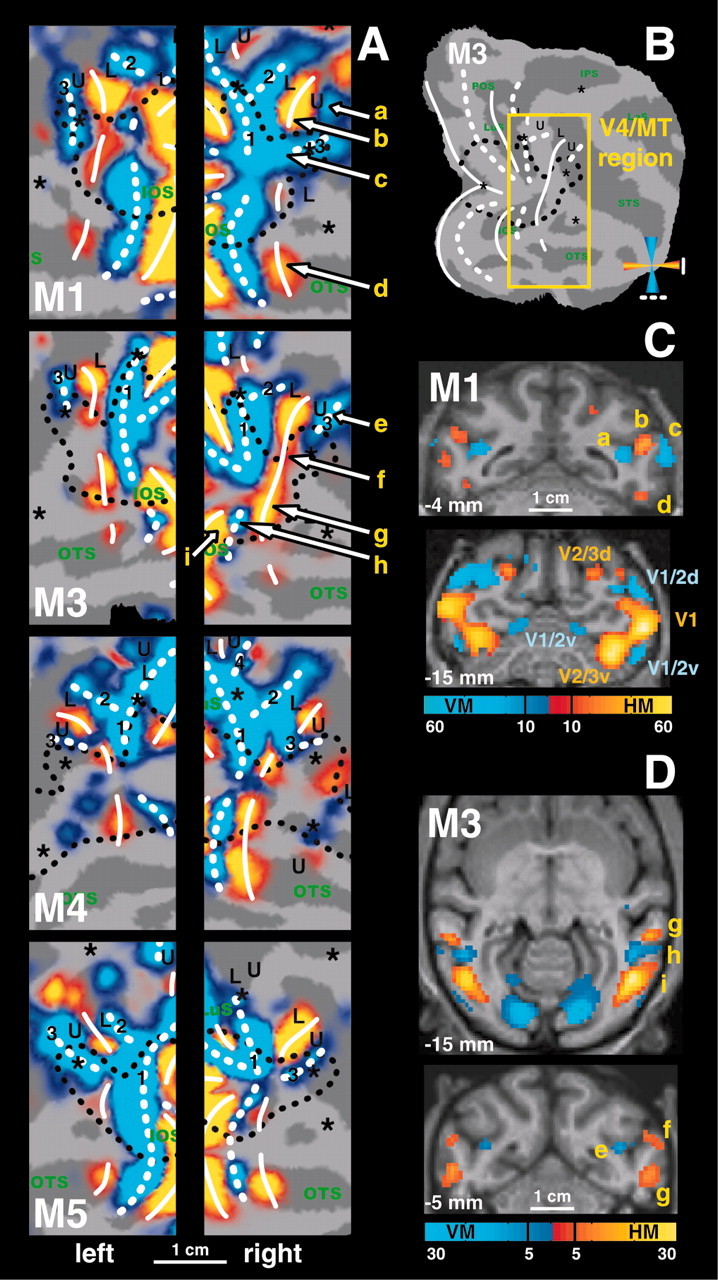
Horizontal and vertical meridian representations in area V4 and neighboring cortex. A, T-score maps (p < 0.05, corrected for multiple comparisons) for horizontal (yellow code) and vertical (blue code) meridian representations are imposed on the flattened cortical reconstructions of the left hemispheres and right hemispheres of the four subjects. Same conventions as in Figure 1. The location of the region of interest is shown in B. Yellow labels and arrows indicate locations shown in the coronal and horizontal brain sections in C and D. C, Coronal brain sections of M1 showing horizontal meridian (yellow code) and vertical meridian (blue code) driven activity. The coronal section at -15 mm can be compared with the one of Figure 5C in the same animal (for the UVF-LVF and the LVF-UVF comparison). D, Horizontal and coronal brain sections of M3.

Figure 4.

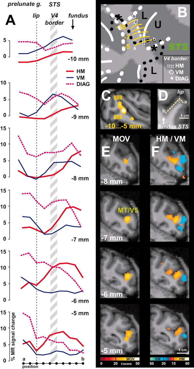
Anterior border of dorsal V4. A, Plots of percentage MR signal change for horizontal meridian (HM, red plot), vertical meridian (VM, blue plot), and the 45°“diagonal” (DIAG, dashed pink plot) stimuli in monkey M1 from the middle of the prelunate gyrus toward the fundus of the STS. The data points were sampled from coronal sections of the prelunate gyrus as indicated by the yellow lines in B-D. Percentage signal changes are relative to the no-stimulus baseline condition. The anterior border of V4 was estimated to be at ∼2-3 mm from the caudal lip of the STS (A, gray hatched zone). B-D, Localization of the coronal slices from which the data, as shown in A, were sampled. One example of a sampling path is shown in a portion of a coronal section in D (from location a → b, as indicated in B,D, and the bottom of A). Samples were taken 1 mm apart from each other. E, Motion-related activity in the same region of M1 (by comparing moving versus stationary random texture patterns) (Vanduffel et al., 2001). The moving stimulus activates MT-V5 in this portion of the STS. F, Horizontal (yellow color code, for the comparison HM-VM) and vertical (blue color-code, for the comparison VM-HM) meridian representations for the same slices as in E.

Figure 5.

Lower and upper visual field representations in the dorsal anterior visual cortex. A, Summary view of the right hemisphere of M3. Same conventions as in Figures 1 and 2. The yellow box indicates the position of the detailed activity maps of all four monkeys as shown in B. B, Upper (blue color code) and lower (yellow color code) visual field representations (p < 0.05, corrected for multiple comparisons) in the dorsal anterior cortex of the eight hemispheres (left hemisphere is on the left, right hemisphere on the right). Yellow labels and arrows indicate locations shown in the brain sections in C and D. C, Upper (blue) and lower (yellow) visual fields representations overlaid onto coronal brain sections of M1. The activities are highly thresholded to obtain good spatial specificity and to visualize the underlying anatomy. Horsley-Clarke coordinates are indicated on the left bottom of each section. Left hemisphere is on the left. Scale bars represent t-scores. D, Sagittal brain section of the left hemisphere of M3; same conventions as C.

Figure 1.

Representation of meridians, central and peripheral, and upper and lower visual field. A, T-score map of horizontal (red-yellow color code: HM-VM) and vertical (blue color code: VM-HM) meridian representations. The activations driven by stimuli confined to the meridians are represented as t-score maps (p < 0.05, corrected for multiple comparisons) on the flattened cortical reconstruction (dark gray: sulci; light gray: gyri). White solid and dashed lines represent the horizontal and vertical meridians, respectively. Labels 1-3 correspond to different VM representations in the region surrounding the prelunate gyrus. B, Significance map for central (red-yellow: central-peripheral VF) and peripheral visual stimulation (blue: peripheral-central VF). Black dashed line indicates the contour of the central 1.5° eccentricity line. Stars indicate additional foveal activations (p < 0.05, corrected for multiple comparisons). C, Significance map for upper (blue: upper-lower VF) and lower (red-yellow: lower-upper VF) visual field representations. “L” and “U” labels indicate the locations of lower and upper field representations. D, E, Summary of visual field maps for M1 (right hemisphere) and M3 (left hemisphere) on the basis of tests as illustrated in A-C. Red labels indicate the visual areas defined by either anatomical location or known visual field representation (V1-4, V3A, LIP) and anatomical location and motion sensitivity (MT-V5, FST). F, G, Plots of percentage MR signal change related to horizontal (red) and vertical (blue) meridian relative to the no-stimulus condition as sampled along the lines indicated in D (a-e) and E (f-j). Error bars represent SEM between the left and right hemispheres. IOS, Inferior occipital sulcus; OTS, occipitotemporal sulcus; STS, superior temporal sulcus; LaS, lateral sulcus; IPS, intraparietal sulcus; POS, parieto-occipital sulcus; LuS, lunate sulcus. (1) The extent of light gray on the anatomical representations could give a misleading estimation of the width of the gyri. A more realistic extent of the gyrus is represented by the yellow ruler in D. This remark holds true for all gyri of all flat maps.

Figure 7.

Eccentricity in area V1. A, Significance map of the activity driven by the [3.5-7]° annulus in M5 (as compared with all other annuli). The iso-eccentricity lines were very similar to those of M1. Black dots represent the sampling points (3 mm ± 0.3) along two lines running parallel to the meridians of area V1. The percentage signal change relative to the no-stimulus condition for the four different stimuli at these points are plotted in B. The locations of 1.5, 3.5, and 7° eccentricity were defined as the intersections of the activity profiles.

t-Score maps were combined and projected onto the flattened cortical reconstruction (at the level of layer 4) of the same animal using Freesurfer software. The flattened representations include the entire occipital pole of the cortex, which was cut anterior to the most rostral tips of the superior temporal sulcus (STS) and intraparietal sulcus. The operculum was split along its representation of the horizontal meridian. This cut extended medially toward the anterior end of the calcarine sulcus. To assess the variability of the maps, we will present detailed data from all eight hemispheres tested.

Results

Representation of meridians and quadrants

Striate and prestriate cortex

At the earliest levels of the visual cortex, transitions between areas are characterized by representations of meridians. Therefore, to identify the borders of these early areas, we first mapped the cortical representation of the horizontal and vertical meridians. The comparison of activity evoked by the vertical and horizontal wedges revealed a stripe-like alternating pattern of higher HM-related (yellow color-coded t-map) and VM-related (blue color-coded t-map) activity (Figs. 1A, 2). The overlying solid (HM) and dashed (VM) white lines correspond to the areal boundaries. These boundaries were derived by combining information from the statistical maps together with local maxima in percentage MR signal change evoked by the horizontal or vertical wedges relative to the no-stimulus condition. This is exemplified in Figure 1, F and G, for monkeys M1 and M3, respectively. The local maxima in percentage signal changes are indicated in Figure 1D-G by the letters a-j. The local t-value maxima (for the VM-HM or HM-VM subtractions), on the other hand, were defined by gradually increasing the threshold of the statistical maps until the local statistical maximum could be visualized. The statistical threshold required to reveal these local maxima differed slightly among the respective positions. This information was combined with the aforementioned local maxima in percentage signal changes (the local t-value maxima and percentage signal change maxima coincided closely, well within the range of our spatial resolution). As one would expect from the electrophysiology, we could define the anterior borders of areas V1 (first VM representation), V2 (second HM), and V3 (second VM) in dorsal and ventral occipital cortex of the four monkeys (Fig. 2).

Figure 2.

Representation of meridians. T-score maps (p < 0.05, corrected for multiple comparisons) of horizontal (red-yellow) and vertical (blue) meridian representations are presented on the flattened cortical reconstructions of the left hemispheres of M1 and M5 and right hemispheres of M3 and M4. Label 4 corresponds to the putative anterior border of V3A. Same conventions as in Figure 1.

Area V4

The large cortical region covering and surrounding the prelunate gyrus is classically assigned to be area “V4” (Zeki, 1977b). Because of the pronounced receptive field scatter, increasing receptive field sizes, and heterogeneity of response properties in this region (Zeki, 1977b; Schein et al., 1982; Maguire and Baizer, 1984; Tanaka et al., 1986; Gattass et al., 1988; Kaas and Lyon, 2001; Pigarev et al., 2002), however, the exact retinotopic organization of this area is still unclear in monkeys. Specifically, the anterior border of dorsal V4 is still controversial because it is not clear whether this area is rostrally completely bordered by a representation of the horizontal meridian (Van Essen and Zeki, 1978; Maguire and Baizer, 1984; Brewer et al., 2002; Pigarev et al., 2002) or whether it is not (Gattass et al., 1988; Brewer et al., 2002; Lyon and Kaas, 2002). To resolve this controversy, we focused on the anterior border of V4.

In agreement with the literature (Gattass et al., 1988), we observed, 7-9 mm rostral to the V3v-V4v border, an HM representation between the inferior occipital sulcus (IOS) and the posterior middle temporal sulcus (PMTS) (Figs. 1A, 2, 3). As described by Boussaoud et al. (1991), this HM representation is discontinuous (see all hemispheres in Fig. 3A) and corresponds to the anterior border of V4v with TEO. In the four monkeys, the dorsal extension of this anterior HM border of V4v curved away from the prelunate gyrus into the STS to become the horizontal meridian between the upper and lower field representation in MT-V5 (Figs. 1C, 3A-C, 4). An independent motion-localizer test (Fig. 4C,E) revealed that at this level in the STS (Fig. 4A) (at levels -6 and -5 mm posterior to the center of the ear canal), the representation of the HM (Fig. 4F, yellow color code) was located within the middle of MT-V5. Therefore, the latter HM representation (Fig 4A) (at levels dorsal to the -6 mm level) cannot correspond to the anterior border of dorsal V4.

Because we found no consistent representation of any principal meridian at the rostral border of anatomically defined V4d, we conducted an additional test (experiment 3) in which we presented stimuli that included not only the meridians but also wedges covering 12° of the visual field centered on the diagonals (tilted 45° clockwise or counterclockwise from vertical; see Materials and Methods). As borne out quantitatively (Fig. 4A), this test revealed that, along the dorsoventral axis, the anatomically defined anterior border of dorsal V4 (in the upper part of the caudal bank of the STS) (Fig. 4A, gray hatched region) is characterized by a gradual transition from the representation of a VM (dorsally), passing through angles that are 45° from vertical, toward a representation of the HM (more ventrally). Thus V4 is bordered anteriorly by an HM representation only near the representation of eccentricities between -5 and -7° (see below for eccentricity test) and farther ventrally (for foveal and upper visual field representations). This gradual transition from the VM toward the HM is illustrated in the plots of the percentage MR signal changes for the principal meridians and the diagonals made along the cortex from the prelunate gyrus toward the fundus of the STS (Fig. 4A). The measurements were taken at 1 mm dorsoventral intervals (in both hemispheres of two monkeys), as illustrated on a flat map and a representative coronal section (Fig. 4B-D, yellow lines). The location of anatomical landmarks (lip of posterior bank of the STS, and the fundus of STS) (Fig. 4D) and the anterior border of anatomically defined V4d (hatched gray) are also indicated on the respective line plots (Fig. 4A). A shift of this “presumptive” V4d border toward either the lip or the fundus of the posterior bank of the STS does not alter our conclusions. The observed transition from a VM toward an HM representation at the anterior border of V4d is in agreement with previous electrophysiological findings (Gattass et al., 1988), although not with a recent anesthetized monkey fMRI experiment (Brewer et al., 2002).

The dorsal border of V4d appears to be a representation of the vertical meridian in six of eight hemispheres (Figs. 1A,2,3A, label 2). The latter VM ran perpendicular to the vertical meridian between V3d and V4d (Figs. 1A, 2, 3A, label 1) (see Discussion). This VM, located between V4d, V3A, and possibly dorsal prelunate area (DP) (see Discussion), has also been described by Gattass et al. (1988, their Fig. 8).

MT-V5 and fundus superior temporal sulcus area

We first used an independent motion-localizer test to functionally define the location of MT-V5 and fundus superior temporal sulcus area. In this test, we compared activity evoked by moving (4°/sec) and stationary random texture patterns 14° in diameter (Vanduffel et al., 2001). Although this test yields an accurate localization of the representation of the central 7° within MT-V5, it does not allow one to define its exact border (because we did not stimulate the peripheral visual field). Yet within functionally defined MT-V5, which fits with its known anatomical location (Vanduffel et al., 2001) (Fig. 4E), a robust retinotopic organization was observed with a horizontal meridian separating ventral upper and dorsal lower visual field representations (Figs. 1C,3A, 4A,F). More ventrally within the STS, area MT-V5 was separated from FST by a representation of a vertical meridian (Figs. 1A, 2, 3A, label 3). Dorsal from MT-V5, another vertical meridian representation was observed in six of eight hemispheres (Fig. 3A, label 2).

V3A

The most straightforward means of distinguishing area V3A from its direct neighbors is on the basis of its representation of the complete contralateral hemifield (Van Essen and Zeki, 1978). By presenting stimuli confined to the upper field, we could identify V3A from its direct neighbors that contain a lower visual field representation only. Indeed, anterior to the large portion of dorsal occipital cortex activated by the lower field stimulus (V1d, V2d, and V3d), an island of cortex in the anectant gyrus that stretched toward the posterior end of the IPS contained an upper field representation (Figs. 1C, 2, 5, label U). Because V3A represents the complete contralateral hemifield, its most caudal part comprises the small strip of cortex with a lower field representation (Figs. 1C, 2, 5, label L) that lies rostral to the anterior border of V3d (VM).

In Figure 3A, this representation of the vertical meridian, lying at the border between V3 and V3A, is illustrated in detail for all hemispheres tested (Figs. 3A,5B, label 1). In all cases, this VM was followed consecutively by a lower and upper field representation (Fig. 5B). In 50% of the hemispheres, a horizontal meridian split these lower and upper field representations (at a statistical criterion of p < 0.05, corrected for multiple comparisons). Anteroventrally, the V3A-V4d border was usually bordered by a vertical meridian (Fig. 2, M4, label 4, and several hemispheres in Figs. 3, 5). Furthermore, the central visual field is represented near the ventral border of V3A (in five of eight hemispheres). In general, the complete hemifield representation in this dorsal portion of the cortex could be reliably used as a fingerprint for V3A. Contrary to the findings of Brewer et al. (2002), however, V3A never covered the entire prelunate gyrus as these authors indicated in their Figure 9 (case H97).

The upper field representation, which covered the anectant gyrus within the anterior bank of the lunate sulcus, extended into the IPS (in six of eight hemispheres) (Fig. 5B). Although this is consistent with the view that V3A also covers the most caudal aspect of the IPS (Tsutsui et al., 2001), adjacent but more anterior areas within this sulcus also seem to have an upper field representation (Figs. 1C, 5B).

Area TEO, lateral intraparietal area, and parieto-occipital area (V6)

Area TEO, located rostral to the anterior HM border of V4v, should be also distinguishable from neighboring cortex by virtue of its representation of the complete contralateral hemifield (Boussaoud et al., 1991). In contrast to V3A, however, the characteristic feature distinguishing TEO from its neighbors is a lower field representation. As marked by the arrow in Figure 1C, we observed such a lower field representation rostral to the anterior HM border of V4v. As in the anesthetized animal (Brewer et al., 2002), the lower field stimulus evoked relatively weak differential MR signals in the region corresponding to TEO. Furthermore, in agreement with the findings of Brewer et al. (2002), we observed a central visual field representation at the most rostral portion of TEO (Figs. 1B, 3, asterisks) in seven of eight hemispheres (M1, M3, M4, and the right hemisphere of M5). Our inability to find a robust retinotopic organization within TEO indicates that neurons with receptive fields driven by upper or lower field stimuli might be heterogeneously distributed [see also Boussaoud et al. (1991)] or that our stimuli were less suitable for driving this region (Hikosaka, 1998).

Additional central visual field representations (Figs. 1, 2, 3, 5, 7, 8, indicated by stars and dashed black lines; see below) were observed at the caudalmost portion of the parieto-occipital sulcus (Fig. 1B, POS, asterisk) and the lateral bank of the IPS. In seven of the eight hemispheres, an extended upper visual field representation emerged, located more posterior relative to this lateral foveal representation, within the IPS (Fig. 5B). These localizations are in agreement with the coarse retinotopic organization of this region (Blatt et al., 1990; Ben Hamed et al., 2001), in which the foveal representation corresponds to the mediodorsal portion of LIP and the more peripheral representation corresponds to the posteroventral portion of LIP (Ben Hamed et al., 2001). Only in M4 (Fig. 5B) did we observe an anteroposterior gradient from the lower to upper visual field representations, as reported by the latter authors.

Summary extrastriate cortex

Figure 1, D and E, summarizes the relative positions of the meridians and the upper and lower visual field representations with respect to the anatomical landmarks for M1 and M3. On the basis of these representations, we could precisely map the borders of areas V1, V2, V3, and V4. Furthermore, we were able to localize all boundaries, except for the anterior border of area MT-V5 and in some hemispheres that of area V3A. Finally, we could define at least one border of area TEO and FST.

Eccentricity mapping

To obtain eccentricity maps throughout the visual cortex, we performed an additional experiment (in M1 and M5) in which we presented four sets of stimuli with texture patterns identical to those used in the meridian and quadrant mapping experiments (see Materials and Methods).

The representation of the central 1.5° is illustrated by the yellow color-coded t-map in Figure 6A. The central visual field stimulus (1.5° radius) activated an elliptical region covering the most lateral portion of the operculum and the anterior tip of the lunate and inferior occipital sulcus. In addition, this ellipse has three extensions. Dorsally it extended along the anterior bank of the lunate sulcus toward V3A (in five of eight hemispheres). Farther rostrally, the foveal representation extended from the prelunate gyrus into the STS (toward MT-V5-FST), and ventrally it covered the prelunate gyrus up to the PMTS (toward TEO) (Fig. 6A). In ventral occipital cortex (V1v, V2v, V3v, and V4v), the 1.5° iso-eccentricity contour ran perpendicular to the areal boundaries. Dorsally, this was also the case for areas V1d, V2d, and V3d. Within dorsal V4, however, this line turned sharply from a caudorostral to a dorsoventral course, because it links the central visual field representation of V3A with that of V4 and MT-V5. As a result, the 1.5° iso-eccentricity line becomes parallel to the anterior border of V3d (that partially abuts V4d) but perpendicular to the V3A-V4 border (Fig. 6, arrows). The results for the 1.5° stimulus could be replicated within the same subject (Figs. 1B,6) and was the same for all animals (Figs. 1B, 2, 3, 5, black dashed lines).

Figure 6.

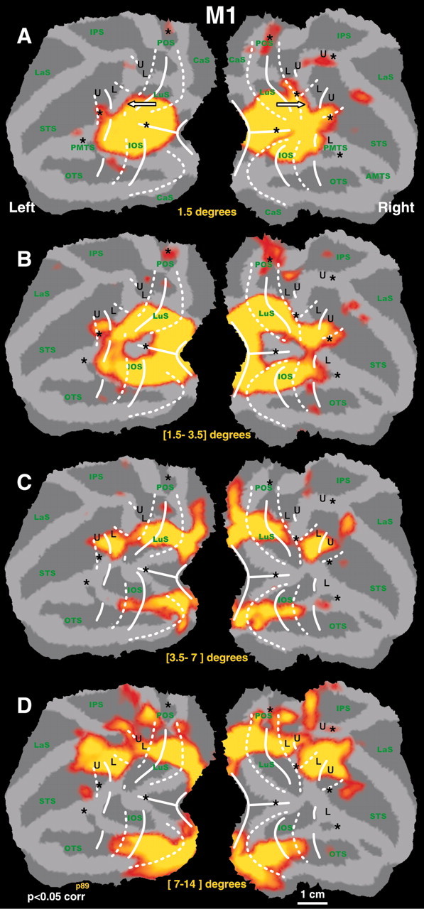
Eccentricity maps for left and right hemispheres of M1. A, T-score maps (p < 0.05, corrected for multiple comparisons) for the central visual field stimulus (1.5° radius). B-D, The activity maps revealed by annuli with a radius of [1.5-3.5], [3.5-7], and [7-14]°, respectively [the respective contrast was always relative to all other annuli types: e.g., (central stimulus) - (all annuli)]. The iso-eccentricity lines, defined by the borders of each activity pattern, were perpendicular to the meridians in the early areas. In dorsal V4, the iso-eccentricity lines run nearly parallel to the areal boundaries (see arrows). Same conventions as in Figure 1.

As the annuli gradually covered larger eccentricities (Fig. 6B-D), the corresponding ring of activity expanded dorsally and ventrally in the operculum, lunate sulcus, IOS, and prelunate gyrus. More peripheral visual stimulation (Fig. 6D) resulted in progressively more dorsocaudal activations within the STS (probably including MSTd) as well as the anterior bank of the parieto-occipital sulcus (corresponding to areas PO/V6/V6A) and posterior parietal cortex including caudal intraparietal sulcus area and 7a. This might reflect the neuronal sensitivity for large and eccentric stimuli in those areas. In a manner similar to the 1.5° eccentricity line, the course of the lines corresponding to larger eccentricities ran perpendicular to the areal boundaries within areas V1, V2, V3, and V4v. Rostral to the vertical meridian marking the border between V3d and V4d, however, the eccentricity lines bent sharply in a ventral direction and became nearly parallel to the V3-V4 boundary [see also Gattass et al. (1988)]. This resulted in a marked compression of mid-eccentricity representations within dorsal V4 (Figs. 6A-C, 7, 8). Interestingly, only stimuli with a radius >7° activated regions in dorsal prelunate, posterior parietal, and dorsal STS cortex.

Using the data from the eccentricity mapping, we could calculate magnification factors for area V1. To this end, we plotted percentage MR signal changes for all eccentricity stimuli tested relative to a no-stimulus baseline condition. The plots were measured from ventral to dorsal locations at 3 mm intervals along two lines that ran parallel to the V1-V2 border as indicated in Figure 7A. We then defined the intersections of the activity profiles from neighboring stimuli (Fig. 7B, vertical dashed lines). The extent of cortex within V1 that was activated by each annulus was defined as the distance between two consecutive intersections. In this way, we determined that the 1.5-3.5° stimulus activated 7 mm, and the 3.5-7° stimulus activated 6.5 mm of cortex. Thus for the average eccentricity of the two annuli (2.5 and 5.25°, respectively), the magnification factors were 3.5 and 1.9 mm/°, respectively. Normalizing all line plots to the maximal activation (Fig. 7, blue curve at level q) yielded very similar ratios: i.e., magnification factors differed <0.1 mm/° compared with those calculated on the basis of non-normalized data. These values are in close agreement with magnification factors reported by Tootell et al. (1988) (3.4 and 2.3 mm/°), Van Essen et al. (1984) (4.0 and 1.7 mm/°) and are near the average of the other studies reported by Tootell et al. (1988) (3.6 and 2 mm/° at 2.5 and 5.3° eccentricity, respectively).

As mentioned, we used the eccentricity data to define the level at which the anterior border of dorsal V4 changed from a diagonal to an HM representation. For M1, we observed this transition between -5 and -7° eccentricity (Figs. 4A,B, 6C). The 1.5° eccentricity lines and the course of the HM were similar in M1, M3, and M4. Thus, although we did not perform the full eccentricity mapping experiments in the latter two monkeys, we can assume with confidence that the representation of the diagonal (as border of V4d) changed to an HM at an eccentricity similar to that in M1. For M5, however, the representation of this HM is much shorter (Fig. 2C) and already bends toward MT-V5 at an eccentricity of approximately -2°. Thus despite some variability, the transition from a representation of a diagonal toward an HM at the anterior border of V4d fits rather well with that documented by Gattass et al. (1988). In some cases (e.g., M5), this transition might occur even closer to the foveal visual field representation (i.e., at smaller eccentricities than -5 to -7°).

Discussion

Areas V1, V2, and V3

The overall retinotopic organization observed in the four monkeys was essentially in agreement with previously described areal boundaries and the representations of quadrants (Daniel and Whitteridge, 1961; Gattass et al., 1981; Van Essen et al., 1984). Area V3 had a mirror representation of area V2, as reported by Gattass et al. (1981, 1988) and Felleman et al. (1997). A longstanding controversy in macaque is whether “V3d” and “V3v-VP” are distinct cortical areas (Burkhalter and Van Essen, 1986; Felleman and Van Essen, 1987) or two parts of a single area with an upper and ventral visual field representation (Gattass et al., 1988; Kaas and Lyon, 2001). We could not document asymmetric retinotopic properties between the two regions, adding evidence to the suggestion that V3d and V3v-VP belong to the same area (Lyon and Kaas, 2002).

Prelunate gyrus and surrounding cortex

Despite a difference in motion sensitivity (Gaska et al., 1988; Tootell et al., 1997; Goebel et al., 1998; Sunaert et al., 1999; Vanduffel et al., 2001), human and macaque V3A showed a remarkably similar retinotopic organization. A characteristic upper and lower visual field representation, separated by a horizontal meridian, was also in agreement with earlier electrophysiological studies (Zeki, 1971, 1977a; Van Essen and Zeki, 1978; Gattass et al., 1988). Similar to our observations, Zeki (1978) described vertical meridians at both the caudal and ventrorostral borders of this area.

A recurrent feature of the anterior bank of the lunate sulcus and prelunate gyrus was the extensive vertical meridian representation. On the basis of anatomical, electrophysiological, and tracer studies (Zeki 1977b; Maguire and Baizer, 1984; Ungerleider and Desimone, 1986; Desimone et al., 1993; Youakim et al., 2001; Lyon and Kaas, 2002), one would expect a vertical meridian exactly where we observed one using our fMRI methods.

The region dorsomedial to the VM representation (Fig. 1A, label 2) receives input from the anterior bank of the parieto-occipital sulcus (Colby et al., 1988), whereas inferotemporal cortex is more heavily connected with the region lying ventrolateral to this VM (Morel and Bullier, 1990; Boussaoud et al., 1991). Furthermore, the dorsomedial but not the ventrolateral region projects to area 7a (Andersen et al., 1990). Thus, it is tempting to ask whether this portion of the prelunate gyrus can be subdivided into a dorsomedial and ventrolateral area divided by a representation of the VM. The existence of different functional properties on the two sides of this VM would further support this idea. In a recent fMRI study, we found sensitivity for three-dimensional structure-from-motion ventrally but not dorsally relative to this VM that is positioned on the prelunate gyrus (Vanduffel et al., 2002). Furthermore, several electrophysiological studies found a high proportion of orientation-sensitive cells dorsomedial to the vertical meridian representation but a much lower proportion ventrolateral to it (Van Essen and Zeki, 1978; Schein et al., 1982; Mountcastle et al., 1987; Youakim et al., 2001). Thus, retinotopically and functionally, as well as anatomically, there is substantial evidence to assign this VM (Fig. 1A, label 2) as dorsal border of V4. The next question is what region the dorsomedial prelunate area might correspond to. In the present study, we could only activate this region by using large peripheral stimuli (Fig. 6D). This finding is in agreement with the electrophysiological results of Tanaka et al. (1986), which showed that the dorsomedial aspect of the prelunate gyrus (their area “PVA”) was driven mainly by large peripheral stimuli. As suggested by Gattass et al. (1988) and Andersen et al. (1990), this dorsal portion of the prelunate gyrus might correspond to area DP.

Ventrolateral to the border with presumed DP, the functional organization of the prelunate gyrus is also complex. On the basis of connection patterns and retinotopy, this region of cortex was originally called V4. Subsequently, several parcellation schemes have been proposed along the caudorostral axis. For example, on the basis of a representation of a horizontal meridian, V4 was further subdivided into V4 proper and V4A (Zeki, 1971; Pigarev et al., 2002) or in rostral (DLr) and caudal (DLc) area DL (Kaas, 1996). At least with the present resolution of our technique, we obtained no evidence for a caudorostral subdivision of dorsal V4. We did find a horizontal meridian at the anterior border of ventral V4 that extended dorsally toward the horizontal meridian, splitting the lower and upper visual field of MT-V5. Thus, we found evidence for a horizontal meridian as an anterior border only for ventral and central V4. In agreement with the electrophysiological maps of Gattass et al. (1988) and the connection patterns of Lyon and Kaas (2002), however, we observed a gradual transition from the VM toward the HM as one moves from dorsal to ventral locations along the anterior V4d border. Exactly as predicted by Gattass et al. (1988), the latter fMRI-defined representation of the HM started at approximately -5to -7° eccentricity (Figs. 4, 8).

Area V4 showed another striking difference between the representations of the upper and lower visual fields in its ventral and dorsal parts, respectively. Although the iso-eccentricity lines were perpendicular to the V3v-V4v border, they ran almost parallel to the V3d-V4d border. This pattern of iso-eccentricity lines is highly comparable with that found in electrophysiological mapping experiments (Gattass et al., 1988) (Fig. 8A) and our earlier fMRI study (Vanduffel et al., 2002, their Fig. 1A). The finding that for at least a portion of the V3d-V4d border (although not for the V3A-V4d boundary) the eccentricity lines run almost parallel to that boundary might indicate that the assumption (as made for the traveling wave method) that the angular and eccentricity representations must lie orthogonal to one another to segment cortical regions into different areas may not be equally valid throughout visual cortex.

One of the most compelling indirect results from this study relates to the “homology” question between human and monkey V4d. In agreement with the electrophysiology and former tracer studies, the present experiment yielded a complex but clear retinotopic organization within monkey dorsal V4. So far, however, not a single human fMRI study has provided any evidence of a robust retinotopic organization within the topological human equivalent of monkey V4d (Bartels and Zeki, 2000; Tootell and Hadjikhani, 2001). Our experiments exclude technique-related explanations for this functional interspecies difference. Furthermore, in New World monkeys, which diverged from the Hominidae much earlier than the Old World monkeys (Preuss, 2003), both dorsal and ventral V4 have a similar retinotopic organization compared with that of V4v in humans and monkeys (Pinon et al., 1998). Together with the present data, this suggests that human and macaque V4d, but not the remainder of early visual cortex, have evolved differently during ∼25 million years of separation.

Despite the fact that a different functional organization between dorsal V4 of human and macaque has been observed, the retinotopic and topological organization of ventral V4 is remarkably similar in the two species; i.e., the caudal border is characterized by a VM, and the rostral border is characterized by an HM. Furthermore, ventral V4 is rather thin and elongated in both species, as opposed to the wide and irregular shaped V4d (or the human V4d topolog). This result suggests that, possibly because of the different evolutionary pathways as suggested above, the upper and ventral counterparts of V4 might not be considered as the lower and upper field representations of a single area (in humans and maybe even in macaques). These differences in retinotopic organization between ventral and dorsal V4 might also indicate that other functional differences between these two regions exist (Tootell and Hadjikhani, 2001).

MT-V5 and FST

In the present study, we first localized area MT-V5 on the basis of its motion sensitivity (Vanduffel et al., 2001). The retinotopic organization within this area closely matched the organization found in previous electrophysiological studies (Van Essen et al., 1981; Desimone and Ungerleider, 1986; Maunsell and Van Essen, 1987) and a recent anterograde tracer study (Lyon and Kaas, 2002). An HM representation separated a dorsal lower field from a ventral upper visual field representation. Furthermore, MT-V5 is dorsally and ventrally bordered by vertical meridian representations (Fig. 8). In human MT-V5, the upper and lower visual field representations are also separated by an HM; however, in contrast to monkey MT-V5, the UVF is represented in the rostrodorsal, and the lower visual field is represented in the caudoventral portion of MT-V5+ (Huk et al., 2002).

Comparison of awake with anesthetized monkey fMRI results

The present results are mostly similar to those observed in a recent anesthetized monkey fMRI study (Brewer et al., 2002). Notable differences between our study and Brewer's are the retinotopic organization and location of V3A and the anterior border of V4. Because the present results are essentially in agreement with electrophysiological findings (Gattass et al., 1988; Felleman and Van Essen 1991), it is unlikely that partial volume effects, attributable to the low spatial resolution (2 × 2 × 2 mm) at a low magnetic field (1.5 T), can explain these differences. Instead, the approximately fivefold increase in contrast-to-noise ratio by using a contrast agent (Vanduffel et al., 2001; Leite et al., 2002) in combination with an awake instead of an anesthetized preparation apparently counterbalanced the gain in signal-to-noise ratio at high field (4.7 T). Another noteworthy feature of MION compared with blood oxygen level-dependent (BOLD) signal is that they arise from capillaries rather than small draining veins, resulting in a crisper localization of the MR signals (Leite et al., 2002). This may have offset the effects of the smaller voxel sizes used in the study by Brewer et al. (2002). The present results also suggest that the combination of an awake animal preparation with high-resolution imaging at high magnetic fields (and stronger gradients) might enable investigators to unravel the retinotopic organization in more extrastriate areas compared with this study.

Conclusion

In general, the fMRI-defined retinotopic organization within single animals is remarkably similar to the existing maps (Felleman and Van Essen, 1991) of monkey cortex. Moreover, except for dorsal V4, our retinotopic maps are in good agreement with the retinotopic organization of human visual cortex. This finding adds evidence to the suggestion that early visual areas (except for V4d) in humans and monkeys might be homologous (Vanduffel et al., 2002). Finally, the significant retinotopic differences between dorsal and ventral V4 might imply different functional roles for these regions. Future fMRI and electrophysiological follow-up studies in the monkey might resolve whether the functional properties of dorsal and ventral V4 are dissimilar enough to consider them as distinct areas.

References

- Andersen RA, Asanuma C, Essick G, Siegel RM ( 1990) Corticocortical connections of anatomically and physiologically defined subdivisions within the inferior parietal lobule. J Comp Neurol 296: 65-113. [DOI] [PubMed] [Google Scholar]
- Bartels A, Zeki S ( 2000) The architecture of the colour centre in the human visual brain: new results and a review. Eur J Neurosci 12: 172-193. [DOI] [PubMed] [Google Scholar]
- Ben Hamed S, Duhamel JR, Bremmer F, Graf W ( 2001) Representation of the visual field in the lateral intraparietal area of macaque monkeys: a quantitative receptive field analysis. Exp Brain Res 140: 127-144. [DOI] [PubMed] [Google Scholar]
- Blatt GJ, Andersen RA, Stoner GR ( 1990) Visual receptive field organization and cortico-cortical connections of the lateral intraparietal area (area LIP) in the macaque. J Comp Neurol 299: 421-445. [DOI] [PubMed] [Google Scholar]
- Boussaoud D, Ungerleider LG, Desimone R ( 1990) Pathways for motion analysis: cortical connections of the medial superior temporal and fundus of the superior temporal visual areas in the macaque. J Comp Neurol 296: 462-495. [DOI] [PubMed] [Google Scholar]
- Boussaoud D, Desimone R, Ungerleider LG ( 1991) Visual topography of area TEO in the macaque. J Comp Neurol 306: 554-575. [DOI] [PubMed] [Google Scholar]
- Brewer AA, Press WA, Logothetis NK, Wandell BA ( 2002) Visual areas in macaque cortex measured using functional magnetic resonance imaging. J Neurosci 22: 10416-10426. [DOI] [PMC free article] [PubMed] [Google Scholar]
- Burkhalter A, Van Essen DC ( 1986) Processing of color, form and disparity information in visual areas VP and V2 of ventral extrastriate cortex in the macaque monkey. J Neurosci 6: 2327-2351. [DOI] [PMC free article] [PubMed] [Google Scholar]
- Chef d'Hotel C, Hermosillo G, Faugeras O ( 2002) Flows of diffeomorphisms for multimodal image registration. Proc IEEE Int S Bio Im 7-8: 21-28. [Google Scholar]
- Colby CL, Gattass R, Olson CR, Gross CG ( 1988) Topographical organization of cortical afferents to extrastriate visual area PO in the macaque: a dual tracer study. J Comp Neurol 269: 392-413. [DOI] [PubMed] [Google Scholar]
- Daniel PM, Whitteridge D ( 1961) The representation of the visual field on the cerebral cortex in monkeys. J Physiol (Lond) 159: 203-221. [DOI] [PMC free article] [PubMed] [Google Scholar]
- Desimone R, Ungerleider LG ( 1986) Multiple visual areas in the caudal superior temporal sulcus of the macaque. J Comp Neurol 248: 164-189. [DOI] [PMC free article] [PubMed] [Google Scholar]
- Desimone R, Moran J, Schein SJ, Mishkin M ( 1993) A role for the corpus callosum in visual area V4 of the macaque. Vis Neurosci 10: 159-171. [DOI] [PubMed] [Google Scholar]
- DeYoe EA, Carman GJ, Bandettini P, Glickman S, Wieser J, Cox R, Miller D, Neitz J ( 1996) Mapping striate and extrastriate visual areas in human cerebral cortex. Proc Natl Acad Sci USA 93: 2382-2386. [DOI] [PMC free article] [PubMed] [Google Scholar]
- Engel SA, Rumelhart DE, Wandell BA, Lee AT, Glover GH, Chichilnisky EJ, Shadlen MN ( 1994) fMRI of human visual cortex. Nature 369: 525. [DOI] [PubMed] [Google Scholar]
- Felleman DJ, Van Essen DC ( 1987) Receptive field properties of neurons in area V3 of macaque monkey extrastriate cortex. J Neurophysiol 57: 889-920. [DOI] [PubMed] [Google Scholar]
- Felleman DJ, Van Essen DC ( 1991) Distributed hierarchical processing in the primate cerebral cortex. Cereb Cortex 1: 1-47. [DOI] [PubMed] [Google Scholar]
- Felleman DJ, Burkhalter A, Van Essen DC ( 1997) Cortical connections of areas V3 and VP of macaque monkey extrastriate visual cortex. J Comp Neurol 379: 21-47. [DOI] [PubMed] [Google Scholar]
- Gaska JP, Jacobson LD, Pollen DA ( 1988) Spatial and temporal frequency selectivity of neurons in visual cortical area V3A of the macaque monkey. Vision Res 28: 1179-1191. [DOI] [PubMed] [Google Scholar]
- Gattass R, Gross CG ( 1981) Visual topography of striate projection zone (MT) in posterior superior temporal sulcus of the macaque. J Neurophysiol 46: 621-638. [DOI] [PubMed] [Google Scholar]
- Gattass R, Gross CG, Sandell JH ( 1981) Visual topography of V2 in the macaque. J Comp Neurol 201: 519-539. [DOI] [PubMed] [Google Scholar]
- Gattass R, Sousa AP, Gross CG ( 1988) Visuotopic organization and extent of V3 and V4 of the macaque. J Neurosci 8: 1831-1845. [DOI] [PMC free article] [PubMed] [Google Scholar]
- Goebel R, Khorram-Sefat D, Muckli L, Hacker H, Singer W ( 1998) The constructive nature of vision: direct evidence from functional magnetic resonance imaging studies of apparent motion and motion imagery. Eur J Neurosci 10: 1563-1573. [DOI] [PubMed] [Google Scholar]
- Grill-Spector K, Kushnir T, Hendler T, Malach R ( 2000) The dynamics of object-selective activation correlate with recognition performance in humans. Nat Neurosci 3: 837-843. [DOI] [PubMed] [Google Scholar]
- Hadjikhani N, Liu AK, Dale AM, Cavanagh P, Tootell RB ( 1998) Retinotopy and color sensitivity in human visual cortical area V8. Nat Neurosci 1: 235-241. [DOI] [PubMed] [Google Scholar]
- Hermosillo G, Chef d'Hotel C, Faugeras O ( 2002) Variational methods for multimodal image matching. Int J Comput Vis 50: 329-343. [Google Scholar]
- Hikosaka K ( 1998) Representation of foveal visual fields in the ventral bank of the superior temporal sulcus in the posterior inferotemporal cortex of the macaque monkey. Behav Brain Res 96: 101-113. [DOI] [PubMed] [Google Scholar]
- Huk AC, Dougherty RF, Heeger DJ ( 2002) Retinotopy and functional subdivision of human areas MT and MST. J Neurosci 22: 7195-7205. [DOI] [PMC free article] [PubMed] [Google Scholar]
- Kaas JH ( 1996) Theories of visual cortex organization in primates: areas of the third level. Prog Brain Res 112: 213-221. [DOI] [PubMed] [Google Scholar]
- Kaas JH, Lyon DC ( 2001) Visual cortex organization in primates: theories of V3 and adjoining visual areas. Prog Brain Res 134: 285-295. [DOI] [PubMed] [Google Scholar]
- Kastner S, De Weerd P, Desimone R, Ungerleider LG ( 1998) Mechanisms of directed attention in the human extrastriate cortex as revealed by functional MRI. Science 282: 108-111. [DOI] [PubMed] [Google Scholar]
- Leite FP, Tsao D, Vanduffel W, Fize D, Sasaki Y, Wald LL, Dale AM, Kwong KK, Orban GA, Rosen BR, Tootell RBH, Mandeville JB ( 2002) Repeated fMRI using iron oxide contrast agent in awake, behaving macaques at 3 Tesla. NeuroImage 16: 283-294. [DOI] [PubMed] [Google Scholar]
- Lewis JW, Van Essen DC ( 2000) Mapping of architectonic subdivisions in the macaque monkey, with emphasis on parieto-occipital cortex. J Comp Neurol 428: 79-111. [DOI] [PubMed] [Google Scholar]
- Logothetis NK, Guggenberger H, Peled S, Pauls J ( 1999) Functional imaging of the monkey brain. Nat Neurosci 2: 555-562. [DOI] [PubMed] [Google Scholar]
- Lyon DC, Kaas JH ( 2002) Evidence for a modified V3 with dorsal and ventral halves in macaque monkeys. Neuron 33: 453-461. [DOI] [PubMed] [Google Scholar]
- Maguire WM, Baizer JS ( 1984) Visuotopic organization of the prelunate gyrus in rhesus monkey. J Neurosci 4: 1690-1704. [DOI] [PMC free article] [PubMed] [Google Scholar]
- Maunsell JH, Van Essen DC ( 1987) Topographic organization of the middle temporal visual area in the macaque monkey: representational biases and the relationship to callosal connections and myeloarchitectonic boundaries. J Comp Neurol 266: 535-555. [DOI] [PubMed] [Google Scholar]
- Morel A, Bullier J ( 1990) Anatomical segregation of two cortical visual pathways in the macaque monkey. Vis Neurosci 4: 555-578. [DOI] [PubMed] [Google Scholar]
- Mountcastle VB, Motter BC, Steinmetz MA, Sestokas AK ( 1987) Common and differential effects of attentive fixation on the excitability of parietal and prestriate (V4) cortical visual neurons in the macaque monkey. J Neurosci 7: 2239-2255. [DOI] [PMC free article] [PubMed] [Google Scholar]
- Pack CC, Berezovskii VK, Born RT ( 2001) Dynamic properties of neurons in cortical area MT in alert and anaesthetized macaque monkeys. Nature 414: 905-908. [DOI] [PubMed] [Google Scholar]
- Pigarev IN, Nothdurft HC, Kastner S ( 2002) Neurons with radial receptive fields in monkey area V4A: evidence of a subdivision of prelunate gyrus based on neuronal response properties. Exp Brain Res 145: 199-206. [DOI] [PubMed] [Google Scholar]
- Pinon MC, Gattass R, Sousa AP ( 1998) Area V4 in Cebus monkey: extent and visuotopic organization. Cereb Cortex 8: 685-701. [DOI] [PubMed] [Google Scholar]
- Preuss TM ( 2003) Specialization of the human visual system: the monkey model meets human reality. In: The primate visual system (Kaas JH, Collins CE, eds). Boca Raton, FL: CRC, in press.
- Preuss TM, Goldman-Rakic PS ( 1991) Architectonics of the parietal and temporal association cortex in the strepsirhine primate Galago compared to the anthropoid primate Macaca. J Comp Neurol 310: 475-506. [DOI] [PubMed] [Google Scholar]
- Rainer G, Augath M, Trinath T, Logothetis NK ( 2001) Nonmonotonic noise tuning of BOLD fMRI signal to natural images in the visual cortex of the anaesthetized monkey. Curr Biol 11: 846-854. [DOI] [PubMed] [Google Scholar]
- Schein SJ, Marrocco RT, de Monasterio FM ( 1982) Is there a high concentration of color-selective cells in area V4 of monkey visual cortex? J Neurophysiol 47: 193-213. [DOI] [PubMed] [Google Scholar]
- Seltzer B, Pandya DN ( 1978) Afferent cortical connections and architectonics of the superior temporal sulcus and surrounding cortex in the rhesus monkey. Brain Res 149: 1-24. [DOI] [PubMed] [Google Scholar]
- Sereno MI, Dale AM, Reppas JB, Kwong KK, Belliveau JW, Brady TJ, Rosen BR, Tootell RB ( 1995) Borders of multiple visual areas in humans revealed by functional magnetic resonance imaging. Science 268: 889-893. [DOI] [PubMed] [Google Scholar]
- Sunaert S, Van Hecke P, Marchal G, Orban GA ( 1999) Motion-responsive regions of the human brain. Exp Brain Res 127: 355-370. [DOI] [PubMed] [Google Scholar]
- Tanaka M, Weber H, Creutzfeldt OD ( 1986) Visual properties and spatial distribution of neurones in the visual association area on the prelunate gyrus of the awake monkey. Exp Brain Res 65: 11-37. [DOI] [PubMed] [Google Scholar]
- Tootell RB, Hadjikhani N ( 2001) Where is “dorsal V4” in human visual cortex? Retinotopic, topographic and functional evidence. Cereb Cortex 11: 298-311. [DOI] [PubMed] [Google Scholar]
- Tootell RB, Switkes E, Silverman MS, Hamilton SL ( 1988) Functional anatomy of macaque striate cortex. II. Retinotopic organization. J Neurosci 8: 1531-1568. [DOI] [PMC free article] [PubMed] [Google Scholar]
- Tootell RB, Mendola JD, Hadjikhani NK, Ledden PJ, Liu AK, Reppas JB, Sereno MI, Dale AM ( 1997) Functional analysis of V3A and related areas in human visual cortex. J Neurosci 17: 7060-7078. [DOI] [PMC free article] [PubMed] [Google Scholar]
- Tsutsui K, Jiang M, Yara K, Sakata H, Taira M ( 2001) Integration of perspective and disparity cues in surface-orientation-selective neurons of area CIP. J Neurophysiol 86: 2856-2867. [DOI] [PubMed] [Google Scholar]
- Ungerleider LG, Desimone R ( 1986) Cortical connections of visual area MT in the macaque. J Comp Neurol 248: 190-222. [DOI] [PubMed] [Google Scholar]
- Van Essen DC ( 2003) Organization of visual areas in Macaque and human cerebral cortex. In: The visual neurosciences (Chalupa L, Werner JS eds). Boston: MIT, in press.
- Van Essen DC, Zeki SM ( 1978) The topographic organization of rhesus monkey prestriate cortex. J Physiol (Lond) 277: 193-226. [DOI] [PMC free article] [PubMed] [Google Scholar]
- Van Essen DC, Maunsell JH, Bixby JL ( 1981) The middle temporal visual area in the macaque: myeloarchitecture, connections, functional properties and topographic organization. J Comp Neurol 199: 293-326. [DOI] [PubMed] [Google Scholar]
- Van Essen DC, Newsome WT, Maunsell JH ( 1984) The visual field representation in striate cortex of the macaque monkey: asymmetries, anisotropies, and individual variability. Vision Res 24: 429-448. [DOI] [PubMed] [Google Scholar]
- Vanduffel W, Fize D, Mandeville JB, Nelissen K, Van Hecke P, Rosen BR, Tootell RB, Orban GA ( 2001) Visual motion processing investigated using contrast agent-enhanced fMRI in awake behaving monkeys. Neuron 32: 565-577. [DOI] [PubMed] [Google Scholar]
- Vanduffel W, Fize D, Peuskens H, Denys K, Sunaert S, Todd JT, Orban GA ( 2002) Extracting 3D from motion: differences in human and monkey intraparietal cortex. Science 298: 413-415. [DOI] [PubMed] [Google Scholar]
- Wandell BA ( 1999) Computational neuroimaging of human visual cortex. Annu Rev Neurosci 22: 145-173. [DOI] [PubMed] [Google Scholar]
- Youakim M, Bender DB, Baizer JS ( 2001) Vertical meridian representation on the prelunate gyrus in area V4 of macaque. Brain Res Bull 56: 93-100. [DOI] [PubMed] [Google Scholar]
- Zeki SM ( 1971) Cortical projections from two prestriate areas in the monkey. Brain Res 34: 19-35. [DOI] [PubMed] [Google Scholar]
- Zeki SM ( 1977a) Simultaneous anatomical demonstration of the representation of the vertical and horizontal meridians in areas V2 and V3 of rhesus monkey visual cortex. Proc R Soc Lond B Biol Sci 195: 517-523. [DOI] [PubMed] [Google Scholar]
- Zeki SM ( 1977b) Colour coding in the superior temporal sulcus of rhesus monkey visual cortex. Proc R Soc Lond B Biol Sci 197: 195-223. [DOI] [PubMed] [Google Scholar]
- Zeki SM ( 1978) The third visual complex of rhesus monkey prestriate cortex. J Physiol (Lond) 277: 245-272. [DOI] [PMC free article] [PubMed] [Google Scholar]